Abstract
Global positioning satellite system (GPS) radio waves that reach the tropical lower troposphere are strongly affected by small-scale water vapor fluctuations. We examine along-the-ray simulations of the impact parameter at every ray integration step using the high-resolution European Centre for Medium-Range Weather Forecasts ERA5 reanalysis as the input model states. We find that disturbances to the impact parameter arise when ray paths go through the top of the sub-cloud layer, where there is a pronounced reduction with increasing height in the humidity, and wet refractivity has a strong local vertical gradient, creating multipath. Additionally, the horizontal gradients of refractivity cause the impact parameter to vary along the ray. The disturbances to the impact parameter are confined to an area about 250 km horizontally and 4 km vertically from the perigee point. Beyond 250 km from the perigee, the impact parameter remains constant. The vertical gradient of refractivity is largest at the top of the sub-cloud layer, usually between 1.5 and 3.0 km, and becomes negligibly small above 4 km.
1. Introduction
Since the proof-of-concept GPS/MET experiment launched in 1995 [1], global positioning satellite system (GPS) radio occultation (RO) has proven to be a valuable atmospheric sounding technique from space, contributing to research and operational weather forecasting [2,3]. The RO technique measures the phase delay of radio waves at two L-band frequencies, which have weak sensitivities to cloud and precipitation. RO measurements also have the highest vertical resolution among satellite observations [4] (Kursinski et al., 1997) as well as many other advantages [2]. Therefore, RO data complement infrared and microwave radiance measurements from meteorological satellites for studying the atmosphere.
GPS radio signals propagate along ray paths that start from a GPS satellite in a medium Earth orbit at an altitude of ~20,200 km through the atmosphere and arrive at a receiver in low-Earth orbit at altitudes of about 400–730 km (Figure 1). When passing through the atmosphere, the radio signals are refracted (bent), depending on the vertical gradient of refractivity along their ray paths. An occultation occurs when a low Earth orbiting (LEO) satellite views a GPS satellite rise or set across the limb. As the radio waves slice through the atmosphere in about 1–2 min, RO measurements (time series of excess Doppler shift) are observed [5]. From these measurements, the bending angle as a function of the impact parameter and the refractivity as a function of pressure can be derived. The largest bending occurs near the perigee where refractivity decreases most rapidly with altitude. In the neutral atmosphere, the atmospheric refractivity (N) is the sum of dry refractivity (Ndry) and wet refractivity (Nwet) as shown in Equations (3) and (4) below. On average Nwet is about 8–9% of the total refractivity [6]. Although wet refractivity is much smaller than dry refractivity, the local vertical and horizontal gradients of wet refractivity can be much larger than the gradients of dry refractivity in the tropical lower troposphere.
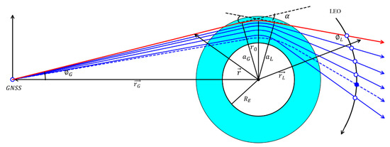
Figure 1.
Schematic representation of GNSS RO ray paths (red and blue solid curves) and a multipath ray (blue dashed curve). Some important parameters characterizing the ray paths are: the bending angle (), a radius vector from the Earth’s center (assumed spherical with radius ) to a point on the ray (), the radius vectors at the GNSS and LEO positions and , the perigee that is defined as the point of the ray that has the shortest distance from the ray to the Earth’s center , the impact parameters at the GNSS and LEO positions and , the ray zenith angle at the GNSS position that is defined as the angle between the radius vector and the tangent direction of the ray at the GNSS position (), and the ray zenith angle at the LEO satellite position that is defined as the angle between the vector and the tangent direction of the ray at the LEO position ().
If the atmospheric refractivity is a function of the radial distance only (spherical symmetry) the impact parameter is constant along a ray path [5]. However, in the tropical lower troposphere where water vapor has small-scale features, the wet refractivity can have strong local gradients, making the refractivity field spherically asymmetric and causing the impact parameter to vary along a ray path. Healy [7] simulated ray paths and Doppler shift values from 54 randomly chosen 6-h model forecasts between November 1998 and October 1999. The model used the same tangent point locations and satellite position and velocity data of a GPS/MET occultation. The Doppler shift values were inverted to obtain the impact parameter at the perigee, bending angle, and refractivity under the spherical symmetry assumption. It was shown that the inverted impact parameter and bending angle at the perigee near the surface can differ from the true values by ~100 m and 3–10%, respectively.
Super-refraction associated with large negative vertical gradients of refractivity (less than −157 N units per km) at the top of moist boundary layers [8,9] caused negative biases in retrieved refractivity [10]. The negative bias, largest below 2 km, with a median value of about 0.5–1% in the tropics decreases upward and is negligible above 4 km [11,12]. The super-refraction also causes multipath propagation, in which radio waves intersect and arrive at a receiver by two or more paths, causing interference. An understanding of where large perturbations occur on RO ray paths is important for understanding RO observations in the tropics.
To examine perturbations to ray paths generated by small-scale water vapor fluctuations in the tropical lower troposphere, a non-local raytracing observation operator can be used to simulate RO ray paths without assuming spherical symmetry [13,14].
In this study, ERA5, with a 0.3° × 0.3° horizontal resolution and 137 levels from the surface to 0.01 hPa [15], is used as input to the two-dimensional (2D) raytracing operator developed by Zou [13]. This was performed to show that ray-path perturbations are associated with along-the-ray variations in the impact parameter and are introduced by strong local vertical gradients of wet refractivity in the vicinity of the perigee point. The high resolution and improved model, observations, and assimilation system of ERA5 compared with other global models make the ERA5 reanalysis more accurate for calculations of the gradients of refractivity (especially the vertical gradient) and for the ray-path integration. However, ERA5 is a hydrostatic model and likely does not resolve extreme small-scale fluctuations of water vapor that occur in the real convective atmosphere.
The work described in the paper extends and substantiates the previous work by Healy (2001) for assessing the impact parameter errors in the middle latitudes to find out where and how large the impact parameter errors are, as well as their relationships to horizontal and vertical gradients of refractivity in the tropical lower troposphere. Major differences between this study and Healy (2001) are as follows: (i) Healy (2001) provided an analysis of the impact of the along-the-track (i.e., tangent direction of the ray path) and across-the-ray (perpendicular to the ray path) gradients of refractivity from mesoscale forecasts in mid-latitudes while we aim at characterizing the statistical analysis of the influence of vertical and horizontal gradients of refractivity in the tropics where the RO impact parameter errors should be larger due to the greater refractivity gradient magnitude; (ii) Healy’s 54 RO cases in different meteorological situations were simulated based on the same occultation geometry (satellite position/velocity data and tangent point locations) while our cases are simulated using the real occultation geometry of co-located COSMIC RO observations; (iii) the 4672 RO samples analyzed in this study are significantly larger than the 54 cases used in Healy, giving more statistical credibility to our results and providing new insights.
This study is organized as follows. Section 2 briefly describes the 2D raytracing operator and input data. Using two individual occultation locations, Section 3 illustrates perturbations of simulated ray paths over local regions with strong vertical gradients of wet refractivity. Statistical results on variations in the geometric heights of simulated ray paths, along-the-ray variations in the impact parameter, impact height and refractivity gradient are provided in Section 4. Section 5 presents conclusions and future plans.
2. Raytracing Operator and Input Data
GPS satellites are equipped with transmitters transmitting radio signals at the highly stable carrier frequencies of and . The electromagnetic rays bend in the atmosphere due to refractivity gradients; the bending angle () is the angle between the ray tangent vectors at the GPS and LEO satellites (Figure 1). Some important parameters characterizing the ray paths are also indicated in Figure 1. The perigee position and the tangent direction are provided by the COSMIC Data Analysis and Archive Center (CDAAC, https://cdaac-www.cosmic.ucar.edu, accessed on 26 September 2021). CDAAC also provides retrievals of bending angle profiles as functions of the impact parameter (a), defined as the distance from this point on the ray to the Earth’s local curvature center multiplied by the index of refraction, i.e., , where is the angle between the tangent direction of the ray and the local radius vector. At the perigee, and . Assuming that the refractive index in the atmosphere is spherically symmetric (), the impact parameter is constant along a ray path.
The propagating electromagnetic ray paths of GPS signals satisfy the following ray trajectory equation [13]:
where is the three-dimensional (3D) radius vector denoting the position of a point on a ray from the Earth’s center, is a parameter associated with the length of the ray (s), defined as , and n is the index of refractivity of the atmosphere defined as:
The refractivity (N) is a function of the pressure (P), temperature (T) through the following relationship [14]:
where P is pressure (hPa), T is temperature (K), ev is water vapor pressure (hPa), N is refractivity (N-unit, a dimensionless quantity), Ndry is dry refractivity (N-unit), and Nwet is wet refractivity (N-unit).
Equation (1) is a second-order ordinary differential equation. It is equivalent to the following first-order equations:
where is a new variable introduced to represent the tangent direction at any point on a ray path. A 2D raytracing operator solves Equation (5) through a ray integration when given an initial condition of (, ) at the perigee position, (, ). The ray integration thus starts from the perigee position () with the tangent direction () to both GPS and LEO satellites. To obtain the ray paths in the coordinates of both geometric height (z) and the impact parameter (a), the raytracing model is integrated, given the ERA5 refractivity. The ray integration uses a variable step size of 2 km or smaller. The bending angle is calculated from the angle between the radius vector and the tangent direction of the ray at the GPS position (), and the angle between the vector and the tangent direction of the ray at the LEO position () as follows:
The impact parameter along the ray path is calculated as
Since the raytracing simulation is carried out in the 2D occultation plane, the part of Doppler shift caused by horizontal gradients perpendicular to the ray path out of the occultation plane cannot be considered by the 2D raytracing operator.
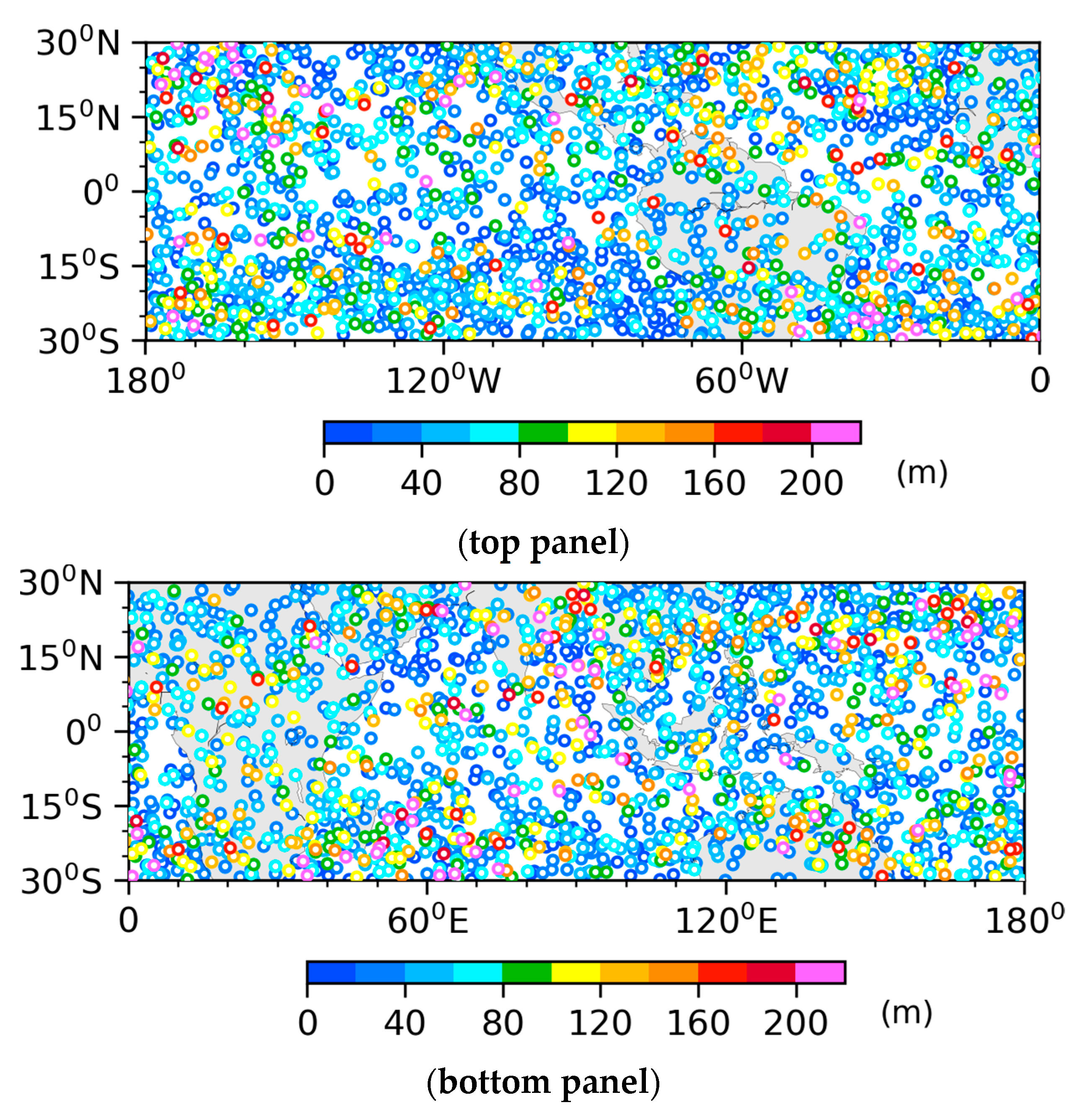
The study period is 1–10 January 2009 characterized by high vertical resolution ERA5 reanalysis. The total number of COSMIC RO profiles is 4627. Figure 2 shows the spatial distributions of the mean locations of all COSMIC profiles within (30°S, 30°N) during this period. Shown in Figure 2 are the maximum values of differences in the impact parameter between the points r0 ± 480 km for simulated rays whose impact heights at the perigee are between 3.35 and 3.45 km. The impact height is defined as the impact parameter minus the radius of curvature of the Earth ( Figure 1), and r0 ± 480 km represents the point on the ray whose horizontal distance from the perigee point of the ray is 480 km. COSMIC occultations with large variations in the impact parameter are randomly distributed in the tropics. The percentage of rays with maximum r0 ± 480 km greater than or equal to 100 m is ~15%.
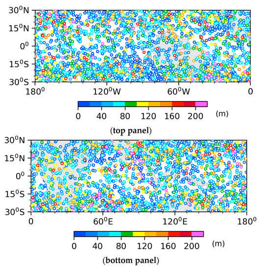
Figure 2.
Spatial distributions of the COSMIC occultations within [30°S, 30°N] during 1–10 January 2009 in the western (top panel) and eastern (bottom panel) hemispheres. The GNSS and LEO satellite positions are to the left and right directions on the x-axis, respectively. The values of maximum are indicated in colors.
Values of the impact parameter, the index of refractivity, and the gradient of refractivity along the ray path are calculated and recorded as the ray integration is carried out for the diagnosis of ray-path perturbations.
3. Examples of Individual Occultation Events
The tropical lower troposphere is characterized from the surface upwards by the planetary boundary layer (PBL), the sub-cloud layer, and the fair-weather cumulus layer [16]. The PBL is the layer below the lifting condensation level and is well-mixed by turbulence. The sub-cloud-layer height is variable, usually between 1.5 and 3.0 km. At the top of the sub-cloud layer, there is a pronounced lapse in the humidity (hydrolapse) and a temperature inversion. The height of the fair-weather cumulus layer is about 4.5 km.
We use the locations of two individual COSMIC RO profiles to illustrate how simulated ray paths vary in the 2D occultation plane, defined as the plane that contains the LEO and GPS satellite positions and the rays’ perigee points. Of interest here is where the altitudes and horizontal distances from the perigee of the simulated rays intersect each other (a condition called multipath), as well as their relationship to locations with large local gradients of wet refractivity. The two locations are (25.08°W, 1.84°S) and (167.09°E, 26.23°N) on 1 January 2009 at 0233 UTC (RO1) and 0201 UTC (RO2), respectively.
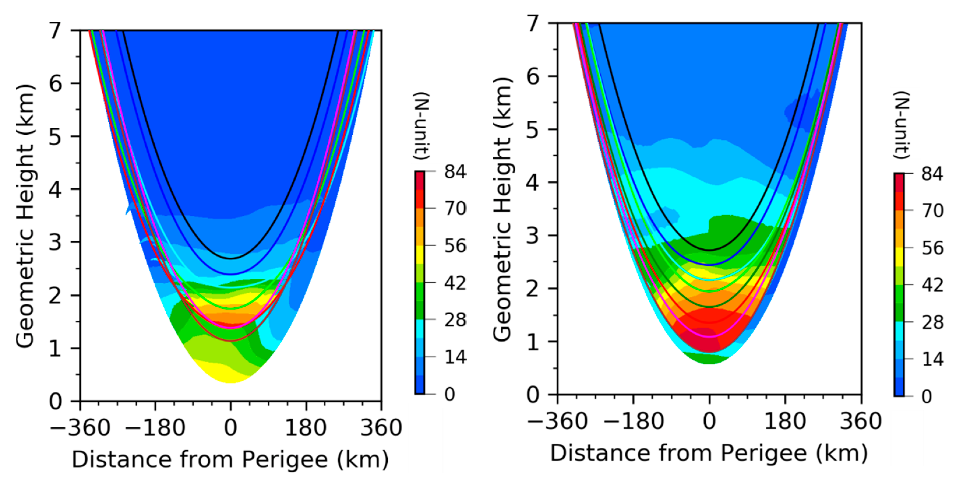
Figure 3 shows the geometric height of eight simulated ray paths and the ERA5 wet refractivity. The simulated rays leaving a GPS satellite position (located at the left side of the x-axis) first go downward to reach the perigee point, and then go upward from the perigee point to the LEO position located to the right of the x-axis. The wet refractivity along the ray paths in the geometric height coordinate would be horizontally distributed if the spherical symmetry is satisfied, which is not the case at low levels within about 180 km horizontal distance from the perigee point for both RO1 and RO2. Here we use wet refractivity for the visualization and analysis because the dry refractivity varies much less (see Figure 13 in [7] and Figure 4b in [17]).

Figure 3.
Variations in the geometric height of eight simulated ray paths (curves) and ERA5 wet refractivity Nwet (N-unit shaded in color) for RO1 (left) and RO2 (right). The GPS and LEO satellite positions are to the left and right directions on the x-axes, respectively. For clarity, every other simulated ray is plotted.
Figure 4 shows the geometric heights of simulated ray paths superimposed on the vertical gradient of ERA5 wet refractivity (Nwet) for RO1 and RO2. A thin vertical layer (~100 m) of large negative vertical gradients of wet refractivity appears at about 2 km near the perigee points of RO1 and RO2. These are around the top of the convective PBL. Several layers of negative and positive vertical gradients of wet refractivity are found within the height range of 1.8 km to 3.8 km. The thin vertical layer of large negative vertical gradients of wet refractivity is associated with the interfacial layer between the moist convective PBL top and the free atmosphere where the main lapse in refractivity occurs due to the large lapse in humidity [18]. In the presence of large local vertical gradients of wet refractivity, the ray paths are not evenly separated in the vertical. Rays with perigee points located below about 2 km are perturbed when they pass through layers with large vertical gradients of wet refractivity, causing these rays to intersect (multipath) in RO1 (Figure 4, top). It is seen that the intersecting rays are associated with large vertical gradients, but these do not reach the condition for super-refraction.
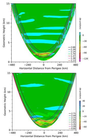
Figure 4.
As in Figure 3 except for vertical gradients of Nwet (N-unit km−1, shaded in color) for RO1 (top panel) and RO2 (bottom panel). The geometric heights of the eight rays at the perigee points (in km) are indicated at the right-bottom corner of each figure.
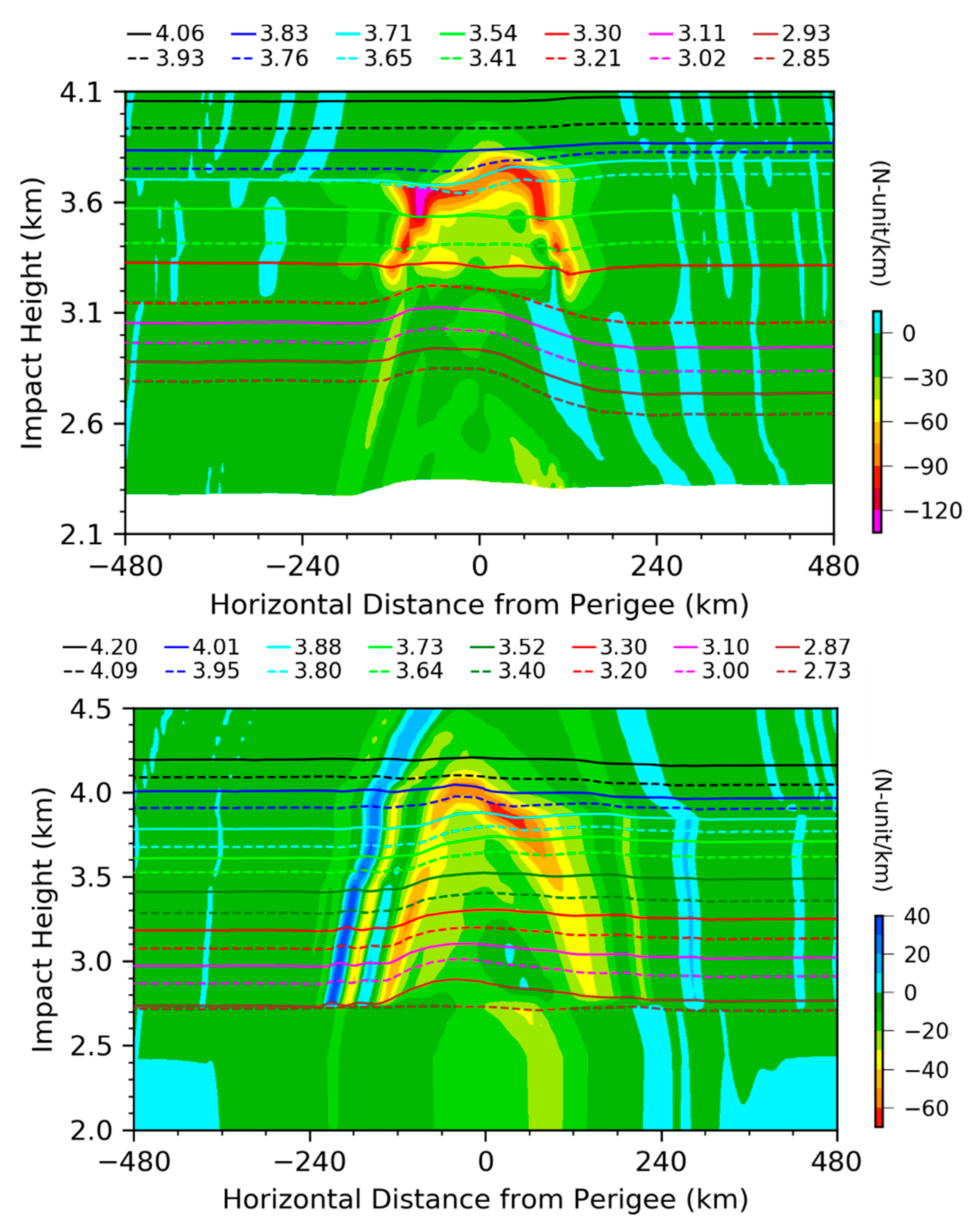
Figure 5 shows an enlarged view of the simulated ray paths vs. the impact height for RO1 and RO2. In a spherically symmetric atmosphere, the impact height of each ray is constant. The impact heights of simulated rays are nearly constant along the rays beyond about 250 km from the perigee point. Closer to the perigee point, variations in impact height occur in areas with large local vertical gradients of wet refractivity, but are usually less than 200 m.

Figure 5.
Impact heights of all 16 simulated ray paths (solid and dashed curves) and vertical gradient of Nwet (N-unit km−1, shaded in color) for RO1 (top panel) and RO2 (bottom panel). The impact heights of rays at the perigee points (in km) are indicated at the top of each panel.
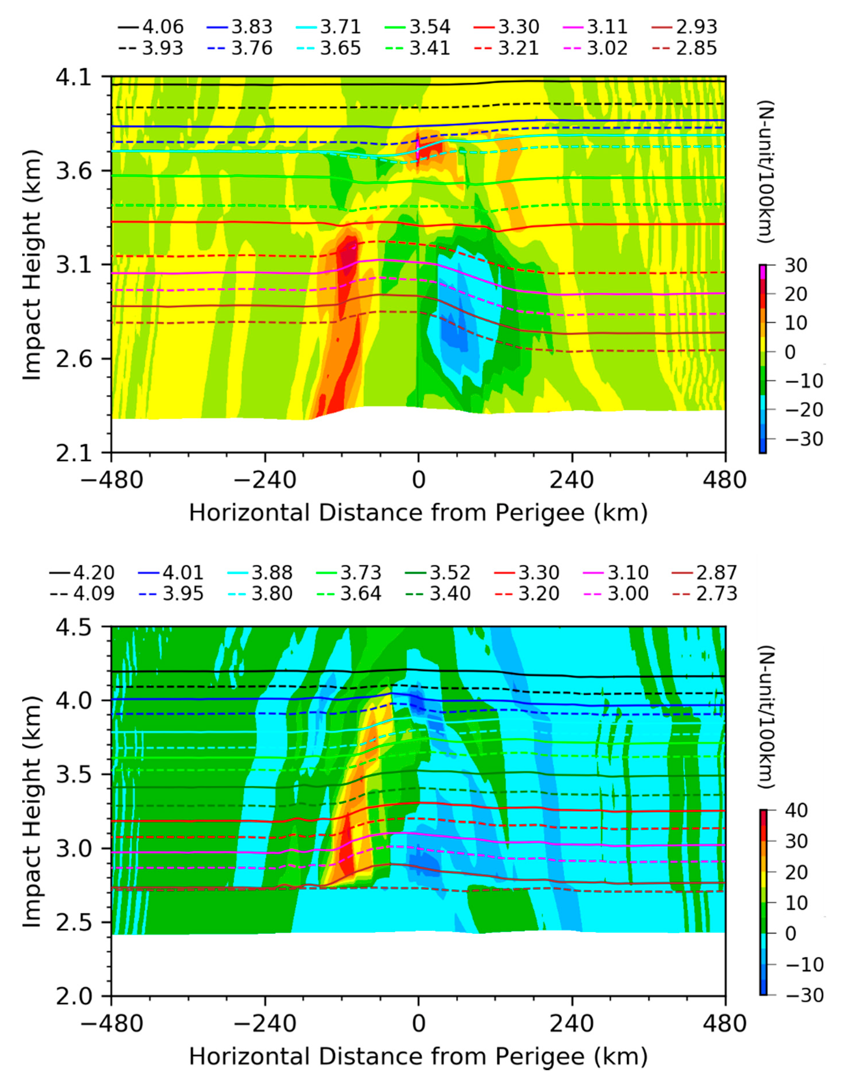
Although a strong vertical gradient can result in a multipath occurrence, which accompanies a local variation in the impact parameter, variations in the impact parameter along the rays are caused by the horizontal gradient of [7]. Figure 6 shows the distributions of horizontal gradients of wet refractivity along the ray paths of RO1 and RO2. Large horizontal gradients of wet refractivity are associated with large vertical gradients of wet refractivity (Figure 4). However, the horizontal gradients (Figure 5) are about two orders of magnitude smaller than the vertical gradients and have broader spatial scales. Large variations in the impact heights occur where horizontal gradients are large.

Figure 6.
Same as Figure 5 except the background colors show the horizontal gradient of Nwet (N-unit. (100 km)−1).
Results in Figure 3 and Figure 6 for the above two RO examples demonstrate that the presence of strong horizontal gradients of refractivity renders the spherical symmetry assumption invalid (Healy, 2001), so that the impact parameter and impact height of a ray passing through the local perturbation is no longer constant.
4. Statistical Results
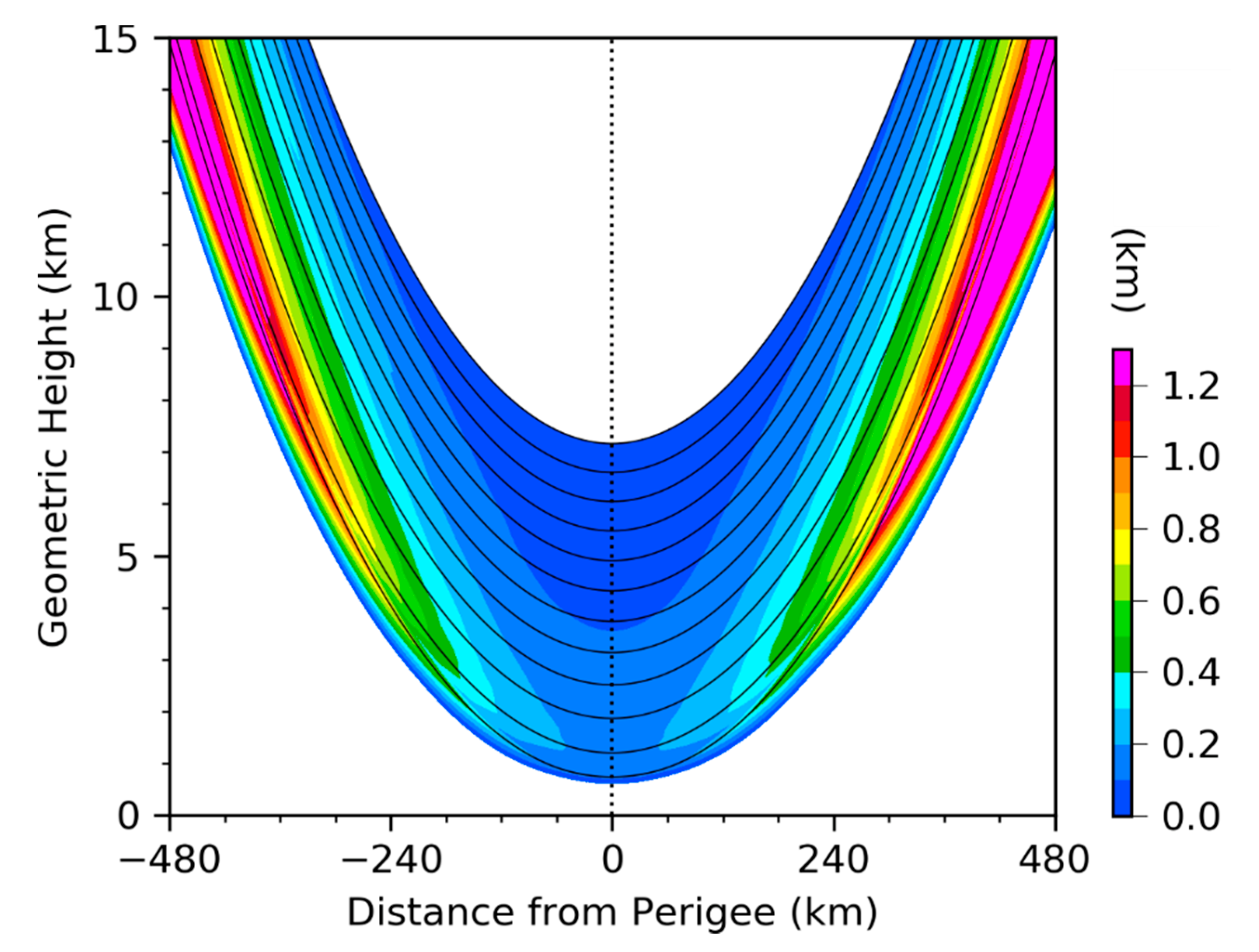
This section presents a statistical analysis of the along-the-ray variations in geometric height and the impact parameter of the 4627 RO simulations. Figure 7 shows the means and standard deviations of simulated ray paths in geometric height coordinates. Since the raytracing model integration starts at the perigee points, the standard deviations of rays’ geometric heights are smallest near the perigee point, larger for low-level rays, and increase with geometric height.

Figure 7.
The means (black curves) and standard deviations (shaded in color) of the geometric heights of simulated ray paths within ±480 km horizontal distances from the perigee points for all 4627 RO simulations. The means and standard deviations are calculated for rays within each of the 100 m intervals of perigee height and 2 km intervals of horizontal distance.
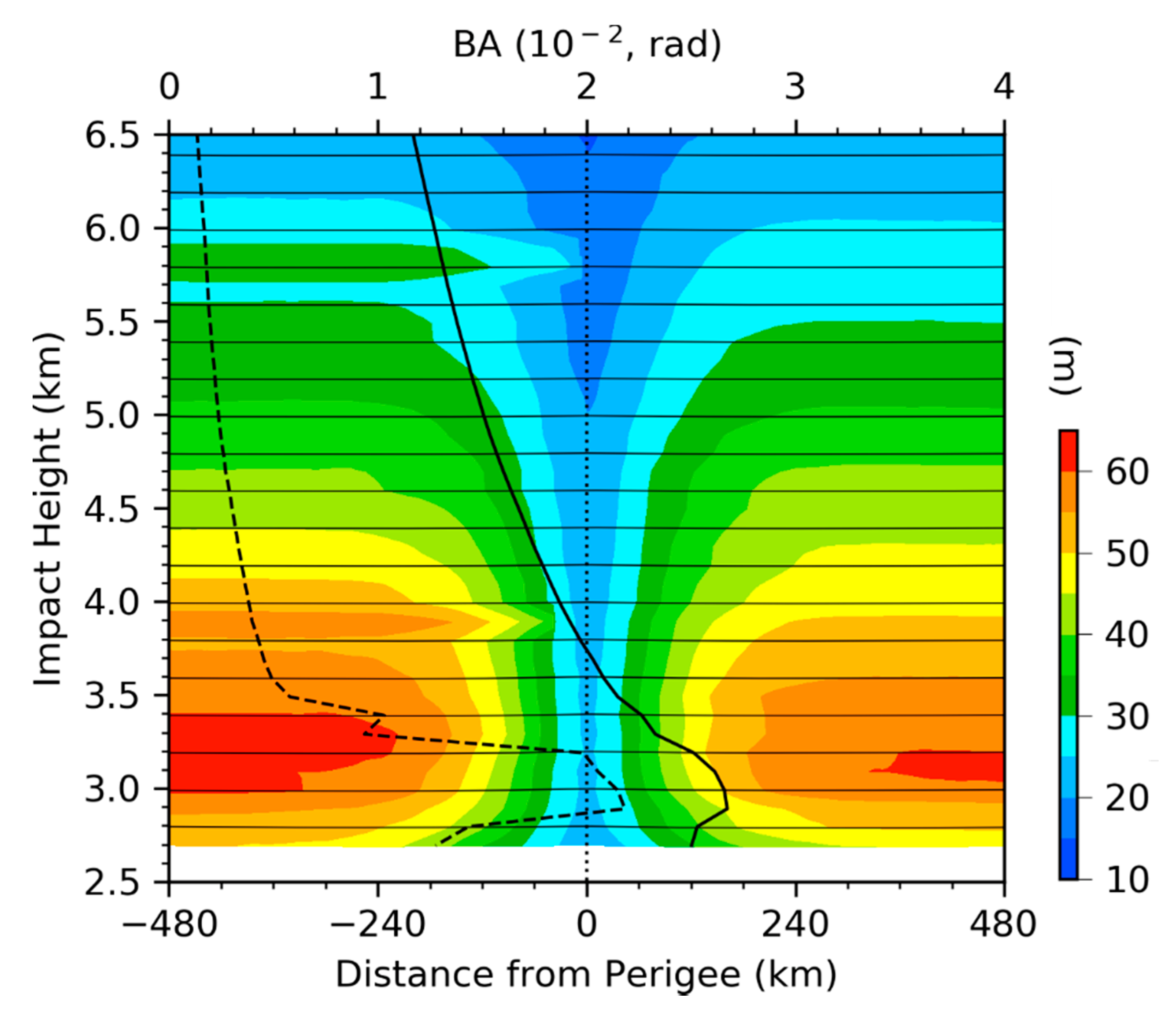
The along-the-ray variations in the geometric height of ray paths are closely related to the variations in the impact parameter along the ray paths. Figure 8 presents the means (thin black curves) and standard deviations (color shading) of the along-the-ray variations in the impact parameter of all simulated ray paths. The means and standard deviations are calculated for rays at each 100 m interval of perigee height and 2 km interval of horizontal distance.
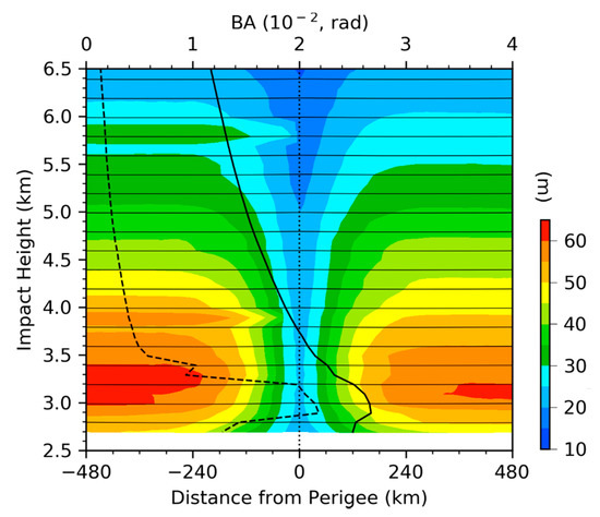
Figure 8.
Variations in the means (thin black curves plotted at every other ray) and standard deviations (color shading) of the impact parameters of simulated ray paths with respect to impact height and horizontal distance from the perigee points, as well as the vertical profiles of the means (thick black curve) and standard deviations (thick dashed black curve) of the simulated bending angles. The means and standard deviations are calculated for rays at each 100 m interval of perigee impact height and 2 km interval of horizontal distance.
The standard deviations of the impact parameter increase from the perigee points to about 250 km from the perigee points, which remain constant as the horizontal distance further increases, and are larger (>30 m) below 5.5-km impact height. This indicates that the large variability in the impact parameter is confined to within 250 km of the perigee points. As expected, there is an extremely large variability of bending angles (45–75%) in the lower troposphere, especially below 3.4 km impact height.
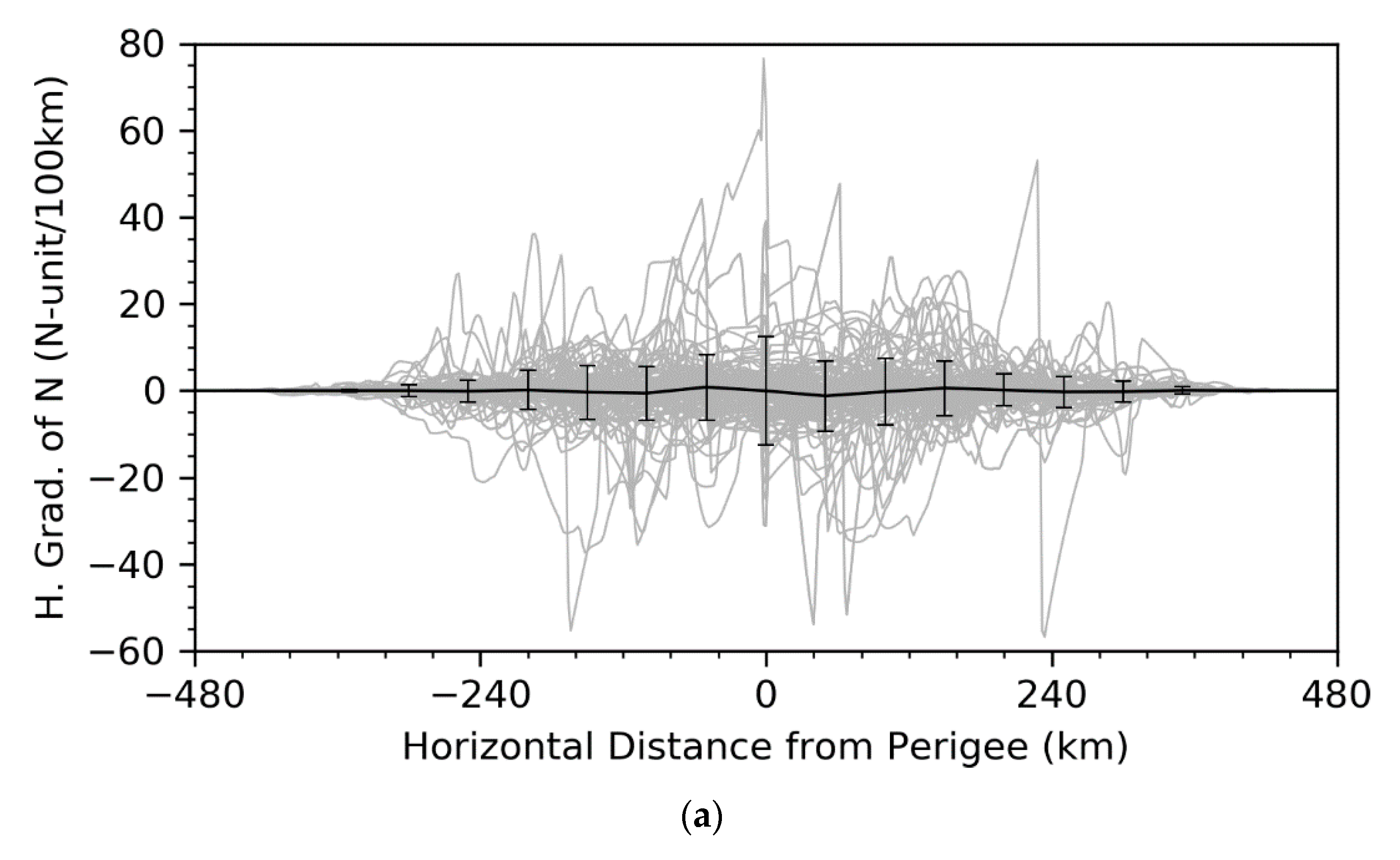
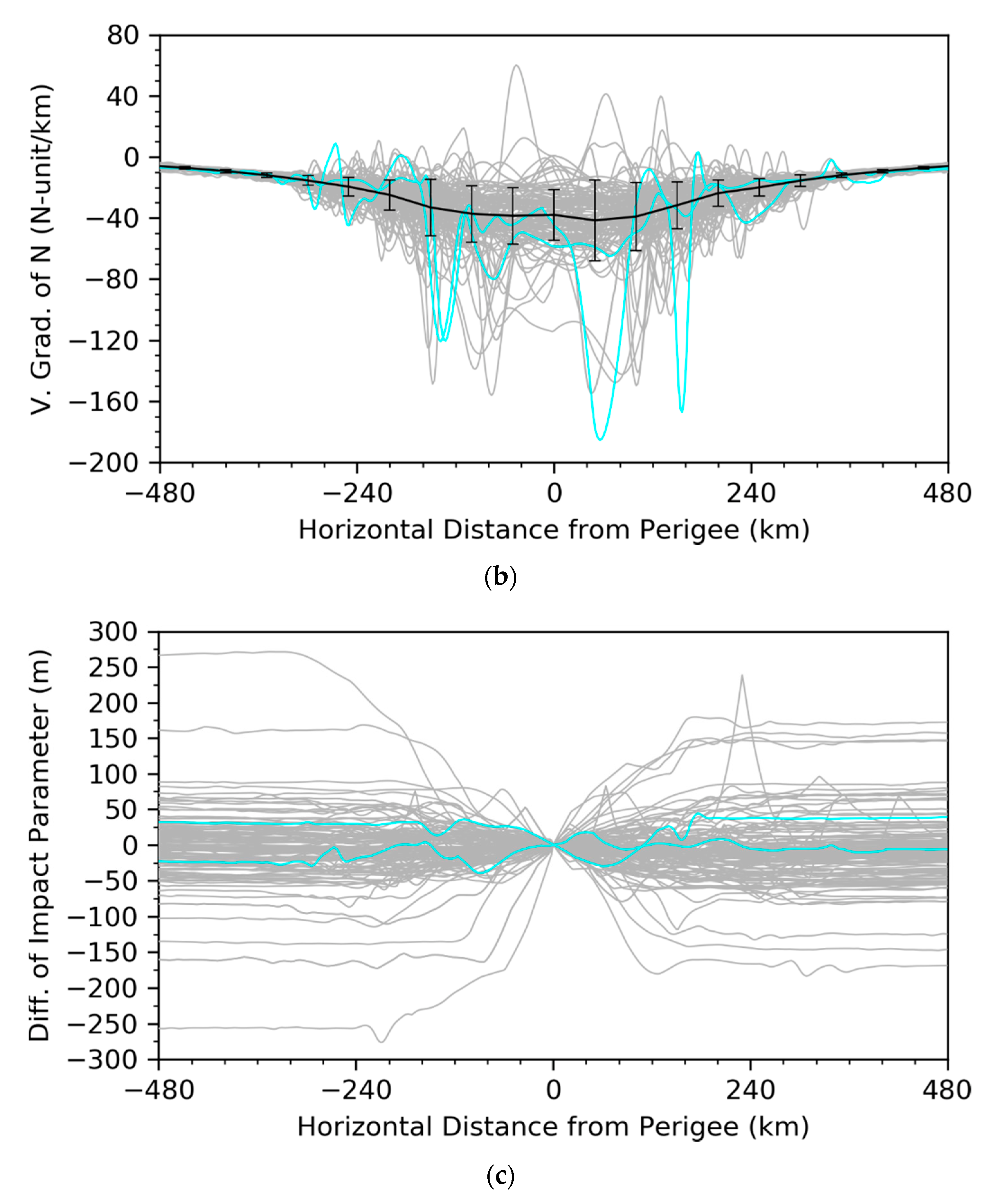
To further show that the large horizontal and vertical gradients of wet refractivity in the tropical lower troposphere correspond to large differences in impact parameters, we calculated the mean and standard deviation of the horizontal and vertical gradients of Nwet at 50 km horizontal-distance intervals, which is shown for rays whose impact heights at the perigee are between 3.399 and 3.401 km as an example (Figure 9). We found large horizontal and vertical gradients of refractivity along the ray paths within 250 km distance from the perigee. The large along-the-ray variations in the impact parameter were also discovered. The variations in the impact parameter along the ray paths are caused by horizontal gradients of refractivity (Figure 9a) along the ray paths, and the impact parameter errors (Figure 9c) are also correlated with the vertical gradients (Figure 9b) as the anomalous horizontal and vertical gradients of refractivity co-exist for the tropical disturbances in the lower troposphere. For rays whose perigee impact heights are around 3.4 km, the vertical gradients at about 120 km from the perigee are much larger than elsewhere, suggesting that the multipath occurs at the preferred altitude (e.g., PBL top).
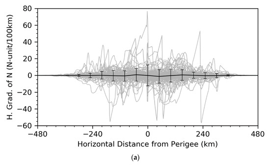
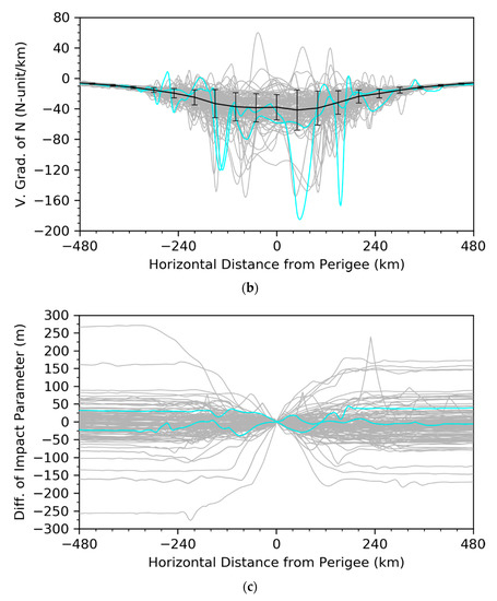
Figure 9.
Along-the-ray variations in (a) horizontal gradients, (b) vertical gradient (gray and cyan curves) and (c) difference of impact parameter from the perigee (a–a0) for rays whose impact heights at the perigee are between 3.399 and 3.401 km for all simulations. Shown in (a,b) are the means (µ black solid curve) and one standard deviations (σ, short black vertical lines) of the vertical gradients of Nwet calculated at 50-km horizontal-distance intervals. The two rays along which there are occurrences of super-refraction (vertical gradient of N is less than −157 N-unit km−1) are shown in cyan in (b,c).
The two rays along which the vertical gradients of refractivity reach the super-refraction condition are indicated in cyan. It is seen that the along-the-ray variations for these two rays are not necessarily largest since the regions of super-refraction are narrow and away from the perigee, confirming that horizontal gradients cause the largest along-the-ray variations in the impact parameter near the perigee.
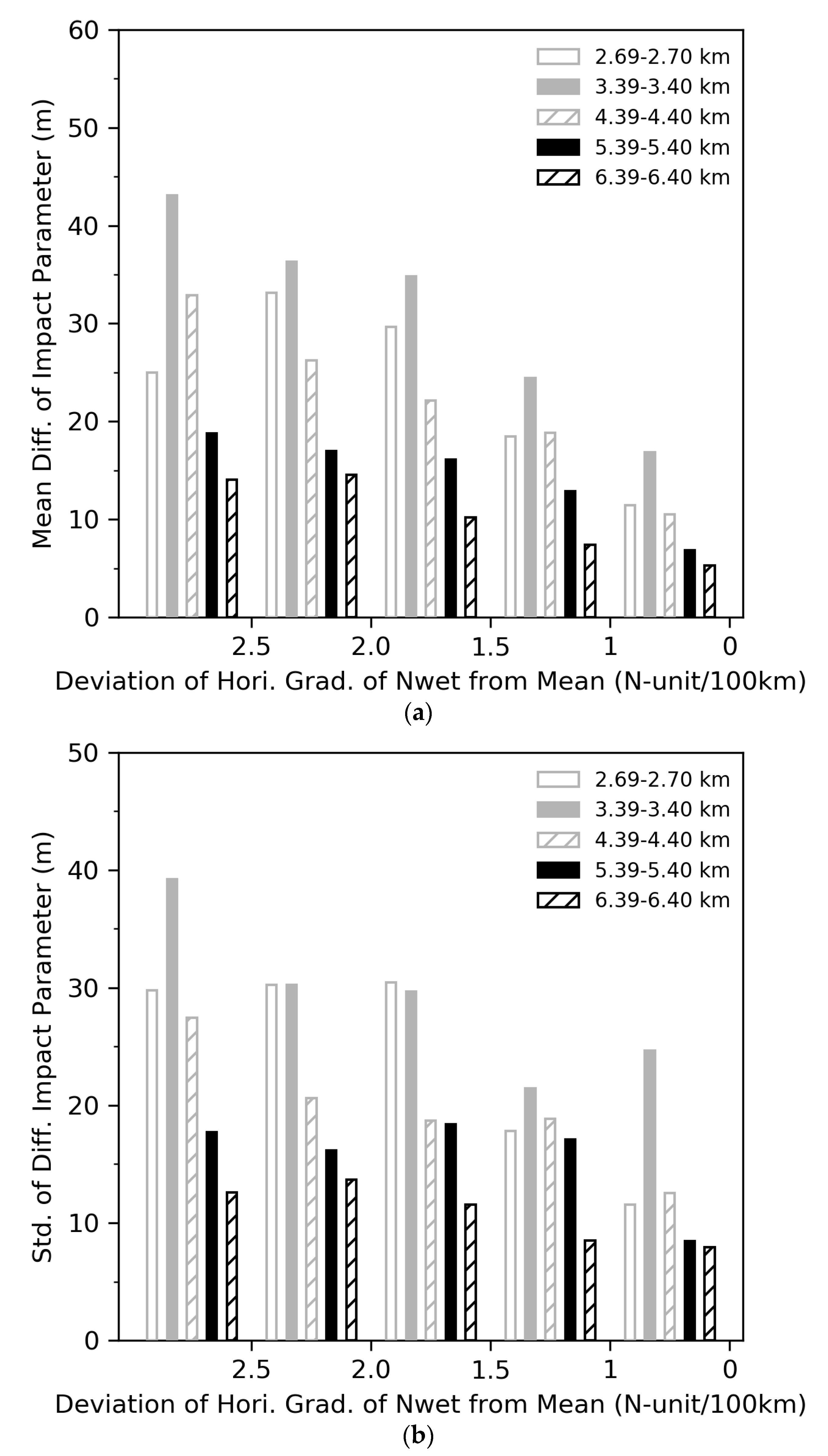
The mean values and standard deviations values of the differences in the impact parameters for rays with different values of the largest vertical gradient of wet refractivity are shown in Figure 10. Both the mean values (Figure 10a) and standard deviations values (Figure 10b) decrease as the largest vertical gradient of wet refractivity decreases between 3.39 and 3.40 km and 6.39 and 6.40 km. The mean values and standard deviations of the differences in the impact parameters for impact heights at the perigee points between 2.69 and 2.70 km are slightly smaller than those between 4.39 and 4.40 km, likely due to larger distances from the perigee points for the rays in the first group (2.69–2.70 km) to pass through the top of the sub-cloud layer than those between 4.39 and 4.40 km (see Figure 3).
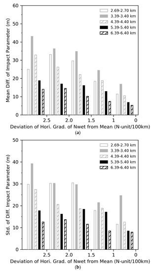
Figure 10.
(a) Mean values and (b) standard deviations of the differences in impact parameter from the mean (see black curve in Figure 9c) normalized by the standard deviations (see the vertical line in Figure 9c) calculated at 50-km horizontal-distance intervals. We divided the differences into 5 groups: with impact heights at the perigee points between 2.69 and 2.70 km (gray hollow bars), between 3.39 and 3.40 km (gray solid bars), between 4.39 and 4.40 km (gray slashed bars), between 5.39 and 5.40 km (black solid bars), and between 6.39 and 6.40 km (black slashed bars).
5. Summary and Conclusions
This study investigates the impacts of small-scale water vapor fluctuations in the GPS radio waves that reach the tropical lower troposphere.
We examined the along-the-ray simulations of the impact parameter at every ray integration step using the high-resolution European Centre for Medium-Range Weather Forecasts ERA5 reanalysis as input model states.
Using two examples, we first illustrated how perturbations are introduced to simulated ray paths by large local gradients of wet refractivity at the top of the sub-cloud layer.
The period chosen for this research study is 1–10 January 2009, characterized by high vertical resolution. The total number of COSMIC RO analyzed profiles is 4627.
Based on the simulated ray paths for all COSMIC occultations within (30°S–30°N), we conducted a statistical analysis of the along-the-ray variations in geometric height, impact parameter, and the total along-the-ray variation in the impact parameter. It was found that simulated ray paths going through the top of the sub-cloud layer characterized by strong local vertical gradient disturbance induces a large jump of the impact parameter. This creates the so-called multipath.
The impact parameter experiences significant variations within the 250 km horizontal distances from the perigee point and remains constant beyond the distances due to the horizontal gradients of refractivity in the tropical lower troposphere. Above 4 km altitude, the impact parameter errors are negligible.
Future work will first examine the relationship between impact parameter and bending angle errors, then develop a quality control based on the gradient-of-wet-refractivity on COSMIC–2 observations, and finally assess their impacts on COSMIC–2 data assimilation and other applications within the latitudinal band (45°S–45°N).
Author Contributions
Data curation, S.Y.; Formal analysis, X.Z.; Methodology, S.Y.; Writing—original draft, S.Y.; Writing—review & editing, X.Z. and R.A. All authors have read and agreed to the published version of the manuscript.
Funding
This research was supported by the National Natural Science Foundation of China (41875032) for Yang and by the NSF-NASA grant AGS-1522830 and NOAA contract 16CN0070 for Anthes.
Data Availability Statement
The COSMIC RO data and the ECMWF ERA5 reanalysis used in this study were downloaded from NCAR’s website at https://www.cosmic.ucar.edu and ECMWF’s website at https://www.ecmwf.int/en/forecasts/datasets/reanalysis-datasets/era5, respectively.
Acknowledgments
We would like to acknowledge the suggestions provided by the reviewers and the editor.
Conflicts of Interest
The authors declare no conflict of interest.
References
- Ware, R.; Exner, M.; Feng, D.; Gorbunov, M.; Hardy, K.; Herman, B.; Kuo, Y.; Meehan, T.; Melbourne, W.; Rocken, W.; et al. GPS sounding of the atmosphere from low earth orbit: Preliminary results. Bull. Am. Meteorol. Soc. 1996, 77, 19–40. [Google Scholar] [CrossRef] [Green Version]
- Anthes, R.A. Exploring Earth’s atmosphere with radio occultation: Contributions to weather, climate and space weather. Atmos. Meas. Tech. 2011, 4, 1077–1103. [Google Scholar] [CrossRef] [Green Version]
- Ho, S.P.; Anthes, R.A.; Ao, C.O.; Healy, S.; Horanyi, A.; Hunt, D.; Mannucci, A.J.; Pedatella, N.; Randet, W.J.; Simmons, A.; et al. The COSMIC-FORMOSAT-3 radio occultation mission after 12 years: Accomplishments, remaining challenges, and potential impacts of COSMIC-2. Bull. Am. Meteorol. Soc. 2020, 101, E1107–E1136. [Google Scholar] [CrossRef] [Green Version]
- Kursinski, E.R.; Hajj, G.A.; Schofield, J.T.; Linfield, R.P.; Hardy, K.R. Observing Earth’s atmosphere with radio occultation measurements using the Global Positioning System. J. Geophys. Res. 1997, 102, 23429–23465. [Google Scholar] [CrossRef]
- Melbourne, W.G.; Davis, E.S.; Duncan, C.B.; Hajj, G.A.; Hardy, K.R.; Kursinski, E.R.; Meehan, T.K.; Young, L.E.; Yunck, T.P. The Application of GPS to Atmospheric Limb Sounding and Global Change Monitoring; JPL Publication: Pasadena, CA, USA, 1994; pp. 37–50. Available online: https://ntrs.nasa.gov/api/citations/19960008694/downloads/19960008694.pdf (accessed on 15 November 2021).
- Yang, S.; Zou, X. Assessments of cloud liquid water contributions to GPS radio occultation refractivity using measurements from COSMIC and CloudSat. J. Geophys. Res. Atmos. 2012, 117, D06219. [Google Scholar] [CrossRef] [Green Version]
- Healy, S. Radio occultation bending angle and impact parameter errors caused by horizontal refractive index gradients in the troposphere: A simulation study. J. Geophys. Res. Atmos. 2001, 106, 11875–11889. [Google Scholar] [CrossRef]
- Sokolovskiy, S. Effect of super-refraction on inversions of radio occultation signals in the lower troposphere. Radio Sci. 2003, 38, 1058. [Google Scholar] [CrossRef] [Green Version]
- Ao, C.O.; Meehan, T.K.; Hajj, G.A.; Mannucci, A.J.; Beyerle, G. Lower troposphere refractivity bias in GPS occultation retrievals. J. Geophys. Res. 2003, 108, 4577. [Google Scholar] [CrossRef] [Green Version]
- Rocken, C.; Anthes, R.; Exner, M.; Hunt, D.; Sokolovskiy, S.; Ware, R. Analysis and validation of GPS/MET data in the neutral atmosphere. J. Geophys. Res. 1997, 102, 29849–29866. [Google Scholar] [CrossRef]
- Xie, F.; Wu, D.L.; Ao, C.O.; Kursinski, E.R.; Mannucci, A.; Syndergaard, S. Super-refraction effects on GPS radio occultation refractivity in marine boundary layers. Geophys. Res. Lett. 2010, 37, L11805. [Google Scholar] [CrossRef]
- Feng, X.; Xie, F.; Ao, C.; Anthes, R.A. Ducting and biases of GPS radio occultation bending angle and refractivity in the moist lower troposphere. J. Atmos. Ocean. Technol. 2020, 37, 1013–1025. [Google Scholar] [CrossRef]
- Zou, X.; Vandenberghe, F.; Wang, B.; Gorbunov, M.; Kuo, Y.H.; Sokolovskiy, S.; Chang, J.C.; Sela, J.G.; Anthes, R.A. A raytracing operator and its adjoint for the use of GPS/MET refraction angle measurements. J. Geophys. Res. Atmos. 1999, 104, 22301–22318. [Google Scholar] [CrossRef] [Green Version]
- Healy, S.B.; Eyre, J.R.; Hamrud, M.; Thépaut, J.N. Assimilating GPS radio occultation measurements with two-dimensional bending angle observation operators. Q. J. R. Meteorol. Soc. 2007, 133, 1213–1227. [Google Scholar] [CrossRef]
- Hersbach, H.; Bell, B.; Berrisford, P.; Hirahara, S.; Horányi, A.; Muñoz-Sabater, J.; Nicolas, J.; Peubey, C.; Radu, R.; Schepers, D.; et al. The ERA5 global reanalysis. Q. J. R. Meteorol. Soc. 2020, 146, 1999–2049. [Google Scholar] [CrossRef]
- Stevens, B.; Brogniez, H.; Kiemle, C.; Lacour, J.-L.; Crevoisier, C.; Kiliani, J. Structure. dynamical influence of water vapor in the lower tropical troposphere. Surv. Geophys. 2017, 38, 1371–1397. [Google Scholar] [CrossRef]
- Zou, X.; Liu, H.; Kuo, Y.-H. Occurrence and detection of impact multipath simulations of bending angle. Q. J. R. Meteorol. Soc. 2019, 145, 1690–1704. [Google Scholar] [CrossRef]
- Garratt, J.R. The Atmospheric Boundary Layer; Cambridge University Press: New York, NY, USA, 1992; p. 316. [Google Scholar]

Publisher’s Note: MDPI stays neutral with regard to jurisdictional claims in published maps and institutional affiliations. |
© 2021 by the authors. Licensee MDPI, Basel, Switzerland. This article is an open access article distributed under the terms and conditions of the Creative Commons Attribution (CC BY) license (https://creativecommons.org/licenses/by/4.0/).