Evaluating the Correlation between Thermal Signatures of UAV Video Stream versus Photomosaic for Urban Rooftop Solar Panels

Abstract

The unmanned aerial vehicle (UAV) autopilot flight to survey urban rooftop solar panels needs a certain flight altitude at a level that can avoid obstacles such as high-rise buildings, street trees, telegraph poles, etc. For this reason, the autopilot-based thermal imaging has severe data redundancy—namely, that non-solar panel area occupies more than 99% of ground target, causing a serious lack of the thermal markers on solar panels. This study aims to explore the correlations between the thermal signatures of urban rooftop solar panels obtained from a UAV video stream and autopilot-based photomosaic. The thermal signatures of video imaging are strongly correlated (0.89–0.99) to those of autopilot-based photomosaics. Furthermore, the differences in the thermal signatures of solar panels between the video and photomosaic are aligned in the range of noise equivalent differential temperature with a 95% confidence level. The results of this study could serve as a valuable reference for employing video stream-based thermal imaging to urban rooftop solar panels.

1. Introduction

The urban solar panels are typically scattered, occupying only 1% of the total roof area in the city [1]. Further, they account for only 10% of the rooftop surface available in the standard single-family house [2], carrying six or fewer panels installed with 1 m width and 1.6 m height [3]. The autopilot is operated by executing pre-defined waypoints according to the specific flight plan for the target area. The target subject to autopilot flight is a certain area with at least several hundreds of square meters (for instance, 30 × 30 = 900 m²) while covering more than four pre-defined waypoints [4]. Therefore, autopilot flight at the urban area needs a certain flight altitude at a level that can avoid obstacles such as high-rise buildings, street trees, telegraph poles, etc.

For this reason, the autopilot-based thermal imaging has severe data redundancy—namely, that non-solar panel area occupies more than 99% of ground target, causing a serious lack of the thermal markers on solar panels. Insufficient thermal markers on solar panels cause the matching failure or mismatch on a single solar panel during building thermal photomosaics, resulting in errors in exterior orientation parameters such as direct measurements of distances, angles, positions, and areas of solar panels [5]. In addition, the unnecessary targets possibly contaminate the thermal signatures of solar panels due to the influence of ambient light from unnecessary targets [5,6].

These insufficient thermal markers can be secured by targeting exclusively solar panels installed at only 1% of the total roof area while guaranteeing a high overlapping rate among the number of video frames. Video has an unusual property and offers several advantages in terms of securing accurate and sufficient key points in thermal imaging of urban solar panels. Unlike the static imagery captured by autopilot flight with pre-defined waypoints, dynamic stereo coverage between individual frames can be accomplished with very intensive overlapping within a single solar panel [7,8,9]. Video-based-thermal imaging can capture the thermal signatures from specifically targeted objects with constant overlapping rates within the confined area [7]. This characteristic of video can complement the data redundancy of traditional thermal imaging captured using autopilot flight for scattered small size solar panels in the urban environment.

Autopilot-based thermal imaging with still imageries has secured a position where it can be used as a standardized procedure to replace in situ visual inspections and I–V curve tests for the inspection of solar panels due to time and cost efficiency [10,11]. In this regard, it could be a benchmark for evaluating the thermal signatures obtained from video mosaic. Regarding UAV-borne video thermal imaging, most studies have evaluated its applicability in view of the real-time detection, classification, and tracking of objects [12,13], for instance, field phenotyping of water stress [14] and fire monitoring [15]. Several sources have evaluated the credibility of thermal signatures obtained from UAV autopilot thermal photomosaics by comparing them with the thermal signatures measured using in situ thermometers [14,16,17]. According to Kelly et al. (2019) [16], the uncertainty of thermal signatures obtained from an autopilot thermal photomosaics is in the range of ±0.5 °C, which is lower than the corresponding uncertainty observed in measurements with in situ thermometers under stable conditions. Other studies have evaluated UAV-borne video in comparison with autopilot-based imaging of solar panels in terms of mapping accuracy. For example, Hwang et al. (2021) found that the 3D coordinates of urban solar panels obtained from autopilot-based video mosaics meet the mapping accuracy requirements recommended by the American Society for Photogrammetry and Remote Sensing (ASPRS) [18].

However, to the best of our knowledge, there are no studies in the literature exploring the correlations between thermal signatures obtained from UAV video and those obtained from autopilot-based photomosaic on urban rooftop solar panels. To examine the suitability of video as a complementary tool of autopilot-based thermal imaging on the scattered urban rooftop solar panels, the video should have adequate thermal sensitivity as the level of autopilot-based thermal photomosaics in detecting the thermal anomaly in solar panels. Therefore, the study aims to explore correlations between thermal signatures of UAV video streams versus photomosaics for urban rooftop solar panels.

2. Method

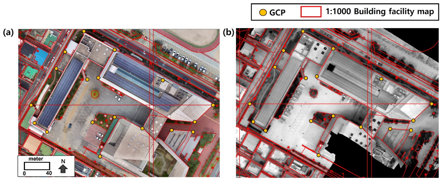
2.1. Experimental Target

The experimental target is in the southeastern part of South Korea, between latitude 35°50′54′′N and longitude 128°32′41′′E (Figure 1). It is in the Dalseong administrative district in the Daegu metropolitan area, the third most populous city in South Korea [19]. Daegu is suitable for solar power generation because it experiences low rainfall and abundant solar radiation, compared with other cities in South Korea [20,21]. The experimental target, Daegu Educational Training Institute, is located in the Gamsam-dong residential area in the city center, which is characterized by diverse land-use patterns, such as commercial, residential, schools, and parks [22]. Solar panels are installed closely along the rooftop boundary on the fifth floor of the institute building. These solar panels have diverse geometric characteristics (tilts, azimuth, and slopes).

Moreover, the rooftop is covered with weather shed, and it houses a ventilator, air conditioner outdoor units, and tiles. Such rooftop surfaces are common in urban areas. In this respect, the selected building represents an ideal study area to comparatively evaluate UAV video streams and photomosaics in the context of thermal imaging of urban rooftop solar panels.

2.2. Acquisition of UAV Thermal Imagery

The UAV video was recorded on 24 August 2020 when the solar zenith angle was the highest (13:00) for avoiding shade and poor weather (for instance, rainfall). The UAV thermal video of solar panels was recorded using a quadcopter DJI Matrice 200 V2 equipped with a DJI Zenmuse XT2 camera (

Table 1. Specifications of UAV and thermal camera.

UAV (DJI Matrice 200 V2)			Camera (DJI Zenmuse XT2)
Weight		4.69 kg	Pixel numbers (width × height)	640 × 512
Maximum flight altitude		3000 m (flight altitude used in this experiment: 80 m)	Sensor size (width × height)	10.88 × 8.7 mm
			Focal length *	19 mm
Hovering accuracy	z (height)	Vertical, ±0.1 m Horizontal, ±0.3 m	Spectral band	7.5–13.5 μm
	x, y (location)	Horizontal, ±1.5 m or ±0.3 m (Downward Vision System)	Full frame rates	30 Hz
Maximum flight speed		61.2 km/h (P-mode)	Sensitivity [NEDT]/Aperture	<0.05 °C, f/1.0

* Focal length of Zenmuse XT2 is fixed at 19 mm while capturing video and still imageries in autopilot mode.; NEDT: noise equivalent differential temperature.

). The solar panels installed in the study area consisted of 72 cells (16 cm in width and 17 cm in height). To detect the thermal information of the cells in the study area, the ground sampling distances (GSDs) of individual thermal UAV video frames should be less than 17 cm. The GSD of a UAV video can be calculated using the focal length of the camera ($F_R$), sensor width of the camera ($Sw$), flight height ($H$), and image width ($imW$), as follows (Equation (1)):

$$\mathrm{GSD}=\frac{Sw\times H\times 100}{F_R\times imW}$$

(1)

As the camera specifications are fixed, flight height is the major contributor to GSD. For this reason, we set the flight altitude to 80 m to achieve the best GSD (7.16 cm) available for detecting individual solar panels in the study area while leaving sufficient space for the UAV to fly freely over the solar panels. Thermal infrared (TIR) video in the form of a sequence-formatted (SEQ) file was captured at 30 frames per s and flight speed of 2.7 m/s.

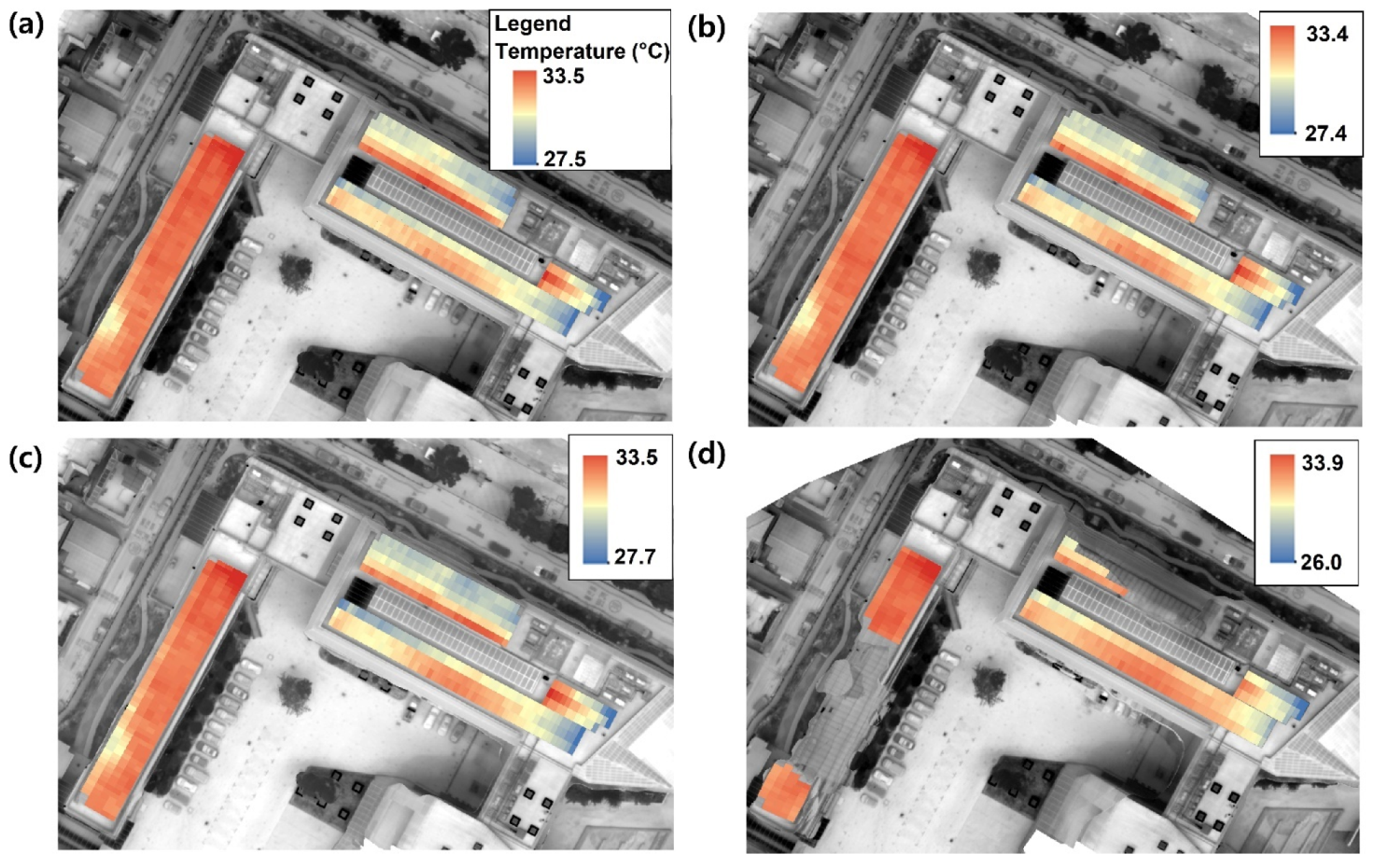
2.3. Video-Based Thermal Frame Mosaic

Raw UAV thermal video frames do not contain geometric information. DJI Matrice 200 V2 and DJI Zenmuse XT2 provide telemetry data for full orientation (position and altitude) in subtitle format (SubRip Subtitle: SRT), along with the recorded thermal video. The time sync function of OSDK V3.8.1 embedded in the flight controller aligns the recording duration of the video, GPS time, and the flight controller clock at 1 Hz. Thus, the SRT file provides second-by-second full orientation data that consist of a number indicating the sequence, Coordinated Universal Time (UTC), and full orientation parameters (GPS coordinates, barometer altitude) acquired from the flight controller during the flight. To extract thermal video imagery from the SEQ video file, we utilized FLIR Tools. The full frame rate of DJI Zenmuse XT2 is 30 Hz (30 frames per second). However, in each recorded second, a few frames appear blurred due to flight vibration and the small aperture of the DJI Zenmuse XT2 (F/1.0). Therefore, the frame intervals of the UAV thermal video captured in this study were set to 15 frames/2 s (overlap: 99%), one frame/1 s (overlap: 97%), and one frame/2 s (overlap: 88%) to reduce noise and guarantee the desired overlapping rate. Autopilot flight was executed over a double-grid path with an overlapping rate of 95%. A photomosaic of individual frames was automatically created using the photogrammetry software Pix4D Mapper and executing the following processes: (1) initial processing (key point extraction, key point matching, camera model optimization, geolocation GPS/GCP); (2) point cloud and mesh generation (point densification, 3D textured mesh); (3) digital surface model (DSM) (photomosaic and index) development.

A structure from motion (SfM) algorithm was applied to establish the camera exposure position and motion trajectory for building a sparse point cloud [23,24,25]. The sparse point cloud was then used for camera calibration, and a multiview-stereo (MVS) was utilized in conjunction with the DSM generation method based on reverse distance weight interpolation to construct a dense point cloud [26,27]. Figure 2 presents the overlap between the thermal photomosaics, with the green areas indicating an overlap of more than five images for every pixel. Mostly, the thermal photomosaics generated using autopilot (hereinafter referred to as the photomosaic) and video imagery is green, except at the borders. The overlap ratios, key points, and matched key points are sufficient for generating high-quality results (Figure 2).

With UAV TIR imagery, identifying ground control points (GCPs) on images is rather perplexing owing to its low spatial resolution and collimation from heat transfer effects. Thermal contrasts can be deducted mostly from the edges of building roofs because the features of the vertical elements around the building are different in terms of thermal infrared radiance [28]. For this reason, we set the edges of the solar panel mounted atop the Daegu Educational Training Institute building as the GCPs (18 points), which were identified from the building vector layer recognized in the 1/1000 digitized building facility map provided by the National Spatial Data Infrastructure Portal, Korean Ministry of Land, Infrastructure, and Transport. As the edge of the Daegu Educational Training Institute building is difficult to access, it is not easy to measure the 3D coordinates (X, Y, Z) with real-time kinematics (RTK) owing to the exterior materials of the building. According to Hwang et al. (2021), the 3D coordinates of the solar panels detected from the VIR video photomosaic built using the RTK-measured GCPs satisfy the mapping accuracy requirements recommended by the American Society for Photogrammetry and Remote Sensing (ASPRS): 3D coordinates (0.028 m) [18]. Hence, we extracted the 3D coordinates of the GCPs from the video visible infrared (VIR) frame mosaic while fulfilling the ASPRS mapping accuracy requirement (Figure 3).

To acquire the solar panel surface temperature (from this point on referred to as the SPST) of individual solar panels, we used individual solar panels’ boundaries to identify the mean SPSTs of individual solar panels.

Table 2. Descriptive statistics of detected SPST (°C) from the solar panels in the thermal frame mosaic obtained from the video images captured using a quadcopter operating on autopilot with a planned flight path.

Category		Autopilot	7.5 Frames/s	1 Frame/s	0.5 Frames/s
SPSTs of solar cells detected in solar panels	Min	26.03	26.02	25.38	24.63
	Max	38.50	38.36	37.51	38.24
	Mean	31.50	31.47	31.47	31.60
	Standard deviation	0.57	0.58	0.60	0.59
Numbers of detected solar panels		645	645	645	359
SPSTs of individual solar panels	Min	27.46	27.44	27.74	26.02
	Max	33.47	33.42	33.46	33.95
	Mean	31.52	31.52	31.53	31.64
	Standard deviation	0.98	0.97	0.98	1.15

shows the temperature pixel values of individual solar modules. The number of solar panels detected seems to be similar between the thermal photomosaic obtained on the basis of autopilot with flight path plan and that obtained from video images (15 frames/2 s, 1 frame/1 s, 1 frame/ frame/2 s). However, the video mosaic processed at 1 frame/2 s has fewer detectable solar panels than the 359 installed solar panels owing to the low quality of the video mosaic with blurred areas (Figure 1). In addition, the SPSTs of the pixels and solar panels are higher (31.60 °C and 31.64 °C) in the thermal mosaics processed at 1 frame/2s than those processed at other frame rates (Table 2).

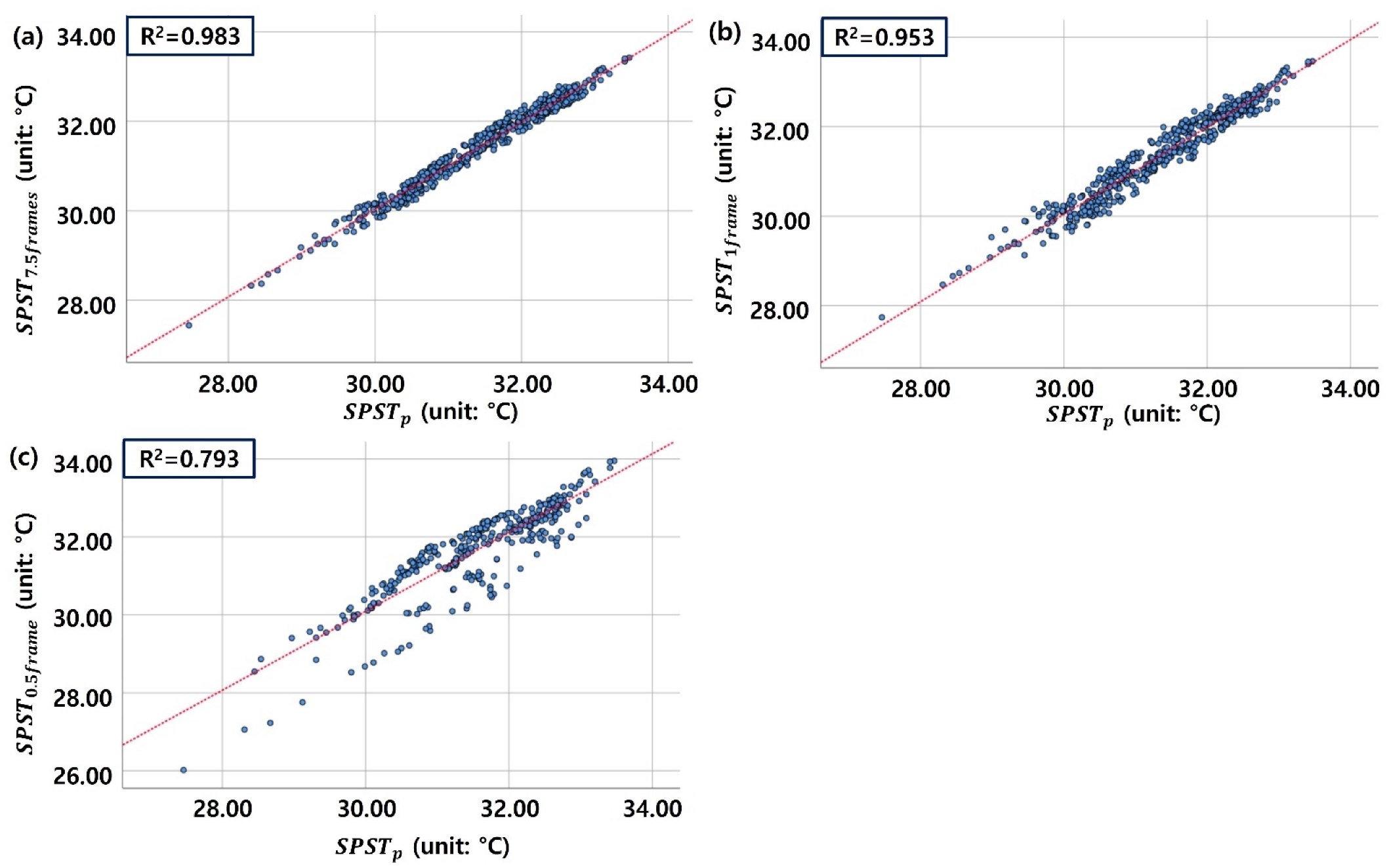
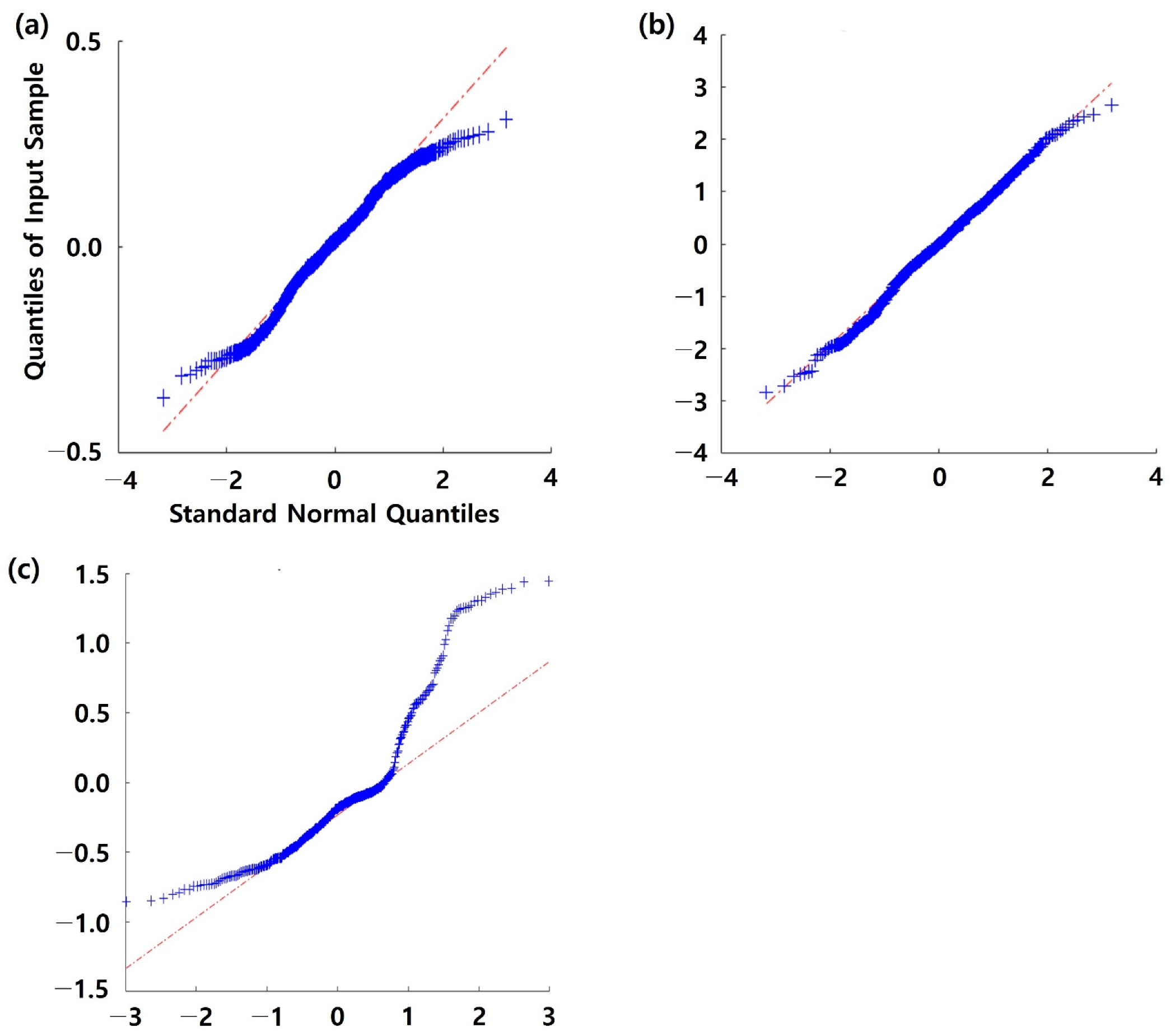
2.4. Evaluating Performance of Video Mosaics in Thermal Deficiency Inspections

This study used a linear regression model to evaluate the relationships and differences between the video versus photomosaic of the same locations by comparing the corresponding SPST values. Linear regression assumes stationary relationships across the study area. Linear regression and Pearson correlation analyses explain the linear relationship between the two variables on the basis of proportional equations [29,30]. Comparative evaluations with linear regression and Pearson correlation can yield the fitness of the SPSTs detected from the UAV video thermal infrared (TIR) frame mosaic (from now on referred to as the video mosaic) and photomosaic. The coefficient and error terms help us determine whether the SPSTs obtained from the UAV video mosaics are over or under-measured, compared with those of the photomosaic. The Pearson correlation indicates that the SPSTs values of the UAV video mosaic and photomosaic have the same directions within the solar panel area.

Given that the coefficient and error terms are close to 1 and 0, respectively, when the Pearson correlation values are higher, the individual SPSTs obtained from the UAV video and photomosaics are similar and can be used as a substitute for the thermal imaging of urban rooftop solar panels. Therefore, the corresponding linear regression models are established as the SPSTs detected from the photomosaics as the dependent variables and video mosaics with different frame intervals. These linear models, which are expressed as Equations (2)–(4), are calibrated using ordinary least squares (OLS) estimation.

$$SPS{T}_p=a_0+a_1\left(SPS{T}_{7.5frames}\right)+{\epsilon }_1$$

(2)

$$SPS{T}_p=b_0+b_1\left(SPS{T}_{1frame}\right)+{\epsilon }_2$$

(3)

$$SPS{T}_p=c_0+c_1\left(SPS{T}_{0.5frame}\right)+{\epsilon }_3,$$

(4)

where $SPS{T}_p$ is the SPSTs obtained from the photomosaic, $SPS{T}_{7.5frames}$ is the SPST obtained from the video mosaic processed at 15 frames/2 s, $SPS{T}_{1frame}$ is the SPST obtained the video mosaic processed at one frame/1 s, and $SPS{T}_{0.5frame}$ is the SPST obtained from the video mosaic processed at one frame/2 s. In Equations (2)–(4), $a_1, b_1, \mathrm{and} c_1$ are coefficients, and ${\epsilon }_1$–${\epsilon }_3$ are random error terms of the residuals. Equations (2)–(4) represent the regression models established using $SPS{T}_{7.5frames}$, $SPS{T}_{1frame}$, and $SPS{T}_{0.5frame}$, respectively, as the explanatory variables and $SPS{T}_p$ as the dependent variable.

A measure of the noise performance of thermal detector systems (sensors) is the noise equivalent differential temperature (NEDT), which is approximately the smallest detectable change in the temperature of a thermal radiation source. NEDT accounts for the influences of all relevant parameters and is an unambiguous measure of the performance of a thermal detector system. NEDT is used as the error covariance, and it influences the assimilation weights compared to other data sources [31]. The NEDT of DJI Zenmuse XT2 is less than 0.05 °C. Given that the differences in the SPSTs obtained from video and photo mosaics are aligned in terms of NEDT, SPSTs detected from the video mosaics have a stable accuracy close to that of the SPSTs detected from the photomosaics. In the case of TIR sensors, sensor noise is estimated by computing the standard deviation of the calibration target measurements [32]. From a statistical viewpoint, the standard deviation is able to appropriately represent the precision of a series of measurements that have a stable mean. As the temperature differences in SPST between the video and photomosaics are aligned in the NEDT range, the SPSTs detected from the video mosaics meet the precision requirements of the measurement. To obtain more detailed information about accuracy, we computed the 95% confidence intervals (CI) of the differences in SPST between the video and photomosaic over the aforementioned NEDT range.

3. Results

Figure 4 and

Table 3. Results of ordinary least squares linear regression between the solar panel surface temperatures (°C) detected from the photo and video mosaic.

Frame Intervals	$\mathit{S}\mathit{P}\mathit{S}{\mathit{T}}_{7.5\mathit{f}\mathit{r}\mathit{a}\mathit{m}\mathit{e}\mathit{s}}$	$\mathit{S}\mathit{P}\mathit{S}{\mathit{T}}_{1\mathit{f}\mathit{r}\mathit{a}\mathit{m}\mathit{e}}$	$\mathit{S}\mathit{P}\mathit{S}{\mathit{T}}_{0.5\mathit{f}\mathit{r}\mathit{a}\mathit{m}\mathit{e}}$
Numbers of solar panels	645	645	359
Unstandardized coefficient (°C)	1.001 *	0.977 *	0.785 *
t-statistic	176.860 *	114.540 *	36.958 *
VIF	1.00	1.00	1.00
Pearson correlation	0.991 *	0.976*	0.890 *
R2	0.983	0.953	0.793
RMSE (°C)	0.14	0.21	0.53
Overlapping rate (%)	99	97	88

*: p-value < 0.01; VIF: variance inflation factor; RMSE: root-mean-square error.

show and summarize, respectively, the results of a regression analysis of the SPSTs detected from video and photomosaic. $SPS{T}_{7.5frames}$ and $SPS{T}_{1frame}$ exhibit strong correlations with $SPS{T}_p$ at shorter frame intervals because the Pearson correlation coefficients are higher than 0.98 (0.98–0.99). Moreover, the model fitness values are extremely high at 0.953–0.983. Furthermore, the unstandardized coefficients, which represent the direction and strength of SPSTs detected from the photo and video mosaic (manual flight), are 0.977–1.001 in shorter frame intervals, indicating a strongly positive (+) linear correlation, that is, the increments in SPSTs are likely to point in the same direction. By contrast, the model for longer frame intervals ($SPS{T}_{0.5frame}$), which has a lower overlapping rate (88%) than that of the photo (95%), shows the lowest value of R² (0.793). Moreover, the coefficient of $SPS{T}_{0.5frame}$ (0.785) is lower than those of $SPS{T}_{7.5frames}$ and $SPS{T}_{1frame}$, indicating that $SPS{T}_{0.5frame}$ tends to be overestimated relative to $SPS{T}_p$ [33]. Identical results can be found when testing the null hypothesis that the coefficients ($a_1, b_1, c_1)$ in the respective models are zero. For this purpose, we computed the respective t-statistics and p-values. The p-value represents the highest error probability at which we cannot reject $H_0$. As all p-values were fairly small, we can reject $H_0$ based on our data. The same result holds for the t-statistics: $\sqrt{n}\ast \overline{X}/S,$ where $\overline{X}$ and S are defined as the sample mean and the sample standard deviation, and n denotes the sample size. In general, higher t-statistic values indicate that we can reject $H_0$, that is, that the corresponding coefficients are more likely to be significant. The precise boundary between significance and insignificance depends on the sample size and Student’s t distribution [34]. However, in general, the benchmark is lower than 3. Hence, given the values in Table 3, the coefficients are highly significant. As the frame intervals become shorter (15 frames/2 s → 1 frame/1 s → 1 frame/2 s), the t-statistic values decrease (176.860 → 114.540 → 36.958). The RMSE increases (0.14 → 0.21 → 0.53 °C) as the frame intervals become shorter (15 frames/2 s → 1 frame/1 s → one frame/2 s). In sum, the shorter frame intervals from the video are more strongly correlated to $SPS{T}_p$.

The thermal UAV video was captured 20 min after the autopilot-based images were captured. SPST was the highest at 14:00 h., even though the solar zenith angle at that time was lower than that at 13:00 h. This is because the solar panels remained heated until 14:00 h, and therefore, SPST peaks at 14:00 h in summer [35]. In this regard, the SPSTs obtained from the video mosaic are higher than $SPS{T}_p$. The difference between the SPSTs at 13:00 h and 14:00 h is less than approximately 1 °C [36]. However, the differences between $SPS{T}_p$ and $SPS{T}_{0.5frame}$ range from −0.86 to 1.45 °C (

Table 4. Differences in SPSTs between photo and video mosaic. The differences are calculated as $SPS{T}_p$ minus SPSTs detected from the video. As the differences are negative (−), the SPSTs detected from the video are higher relative to $SPS{T}_p$.

Frame Intervals		$\mathit{S}\mathit{P}\mathit{S}{\mathit{T}}_{7.5\mathit{f}\mathit{r}\mathit{a}\mathit{m}\mathit{e}\mathit{s}}$	$\mathit{S}\mathit{P}\mathit{S}{\mathit{T}}_{1\mathit{f}\mathit{r}\mathit{a}\mathit{m}\mathit{e}}$	$\mathit{S}\mathit{P}\mathit{S}{\mathit{T}}_{0.5\mathit{f}\mathit{r}\mathit{a}\mathit{m}\mathit{e}}$
Number of solar panels	Negative (−) difference with $SPS{T}_p$	293	323	268
	Positive (+) difference with $SPS{T}_p$	352	322	91
Temperature difference (°C)	Min	−0.366	−0.604	−0.855
	Max	0.310	0.563	1.446
	Mean	0.007	−0.005	−0.106
	Sum	4.357	−3.283	−38.02
	Standard deviation	0.14	0.21	0.52

). These differences are excessive, even when we consider the time lag during shooting. This tendency can be ascribed to differences in the numbers of key points as thermal markers.

In a UAV image, the radial fall-off brightness is away from the image center because of the so-called vignetting effect caused by optical transmission problems [37]. The spatial transmissivity of a vignetted image is normalized to a maximum value of 1. Classically, a camera transmits reduced illumination from the center of an image toward the edges. Thus, the image transmissivity in the center is 1, and it is smaller than 1 toward the image borders. This vignetting effect attenuates the thermal signatures at the edges relative to the actual values owing to the reduced transmissivity and increases signal-to-noise ratio (SNR) of thermal signatures at the edges of thermal images. The Pix4D Mapper software package applies a vignetting polynomial to correct the vignetting effect by modeling the camera optics with the coefficients included in the image headers [16,38,39]. In generating a thermal mosaic, the matched points among the images are calculated using the mean values of the matched key points. This helps one to derive results similar to those when the image edges are excluded. In general, SNR improves drastically by averaging a greater number of frames. The lower overlapping rates between reference frames in mosaics reduce the number of matched key points. An insufficient number of key points leads to the generation of biased thermal signatures with uncorrected vignetting effects. Therefore, to ensure that the quality of thermal signatures obtained from video frames is consistent with those from photos, the video mosaic must use frames with intervals that satisfy or exceed the overlapping rates achieved with autopilot-based imaging.

Table 5. Comparative evaluation of point cloud between video versus photomosaic.

Frame Intervals	2D Key Point Observations	Matched 2D Key Points Per Image (Mean)	Average Density * (/m3)	Area Covered (ha)	Flight Duration (m:s)
$SPS{T}_p$	1,038,092	2749	5.3	4.69	28:00
$SPS{T}_{7.5frames}$	932,947	3571	21.10	1.99	02:09
$SPS{T}_{1frame}$	571,406	3019	15.76	1.85	02:09
$SPS{T}_{0.5frame}$	161,712	1902	13.28	1.34	02:09
Longer frame intervals (15 frames/2 s → 1 frame/1 s → 1 frame/2 s) have lower overlapping rates (99 → 97 → 88%), fewer matched 2D key points per image (3571 → 3019 → 1902), and average density (21.10/m3 → 15.76/m3 → 13.28/m3). $SPS{T}_p$ has lower overlapping rates (95%), the number of matched 2D key points (2749), and average density (5.3/m3) compared with $SPS{T}_{7.5frames}$ and $SPS{T}_{1frame}$ having smaller covered areas.

* Average number of 3D-densified points obtained for the project per cubic meter.

shows that video-based thermal imaging secures approximately three to four-fold numbers of 3D-densified points (15.76–21.0/m³) on the solar panels than on the photo (5.3/m³). Since the photomosaics include the 99% of unnecessary targets of the non-solar panel (4.69 ha) than the video (1.34–1.99 ha), it has the larger 2D key point observations (1,038,092) than video (161,712–932,947). This study was implemented at a public educational facility covered by a large number of solar panels. More than 80% of the roof area in this facility is covered with 645 solar panels, not likely for typical urban solar panels, which account for only 10% of a typical roof area [2]. In other words, the number of 3D-densified points per m³ would be much less in autopilot-based thermal imaging for typical urban solar panels. Nonetheless, this study experimentally validated that the video-based thermal imaging could secure 3D-densified points required in the process of building thermal video mosaics, with the higher overlapping rates and the shorter flight duration.

4. Discussion

The temperature differences between $SPS{T}_{\mathrm{p}}$ and $SPS{T}_{7.5frames}$ range from −0.366 to 0.310 °C, meaning that the differences between the two values are comparatively low in terms of standard deviation (0.14 °C) and mean value (0.007 °C), compared with the temperature difference between $SPS{T}_{1frame}$ and $SPS{T}_{0.5frame}$. Therefore, the SPSTs detected from video mosaics processed at 15 frames/2 s are well aligned with the SPSTs detected from the photomosaics.

To explore the accuracy of the SPSTs detected from video mosaics relative to those of the SPSTs detected from the photo, we computed the 95% confidence intervals (CI) for the abovementioned temperature differences. For this purpose, we first checked whether our sample data followed the Gaussian distribution. This assumption would allow us to compare our results with those of other studies because the Gaussian CI formula has been widely used in the literature. The Jarque–Bera test, which is a rather sensitive test, rejected the hypothesis that the data were Gaussian (maybe source, maybe not). However, as we only require approximate values, we compared the estimated kernel densities with the exact Gaussian density. Figure 5 presents the respective plots for all three temperature differences between $SPST$ versus $SPS{T}_{7.5frames}$, $SPS{T}_{1frame}$ and $SPS{T}_{0.5frame}$. From this figure, it can be inferred that the Gaussian assumption is more or less justified for the temperature differences of $SPS{T}_{7.5frames}$ and $SPS{T}_{1frame}$ against $SPS{T}_{\mathrm{p}}$ but not for the temperature differences between $SPS{T}_{0.5frame}$ and $SPS{T}_{\mathrm{p}}$.

This tendency was observed in the Gaussian tests as well (Figure 6). Kernel density estimation is essentially a non-parametric estimate of the probability density. The stronger the similarity between kernel density and theoretical density, the closer the dataset’s distribution to the theoretical distribution. The kernel density measured from the differences in SPSTs between the video ($SPS{T}_{7.5frames}$, $SPS{T}_{1frame}$) and photomosaics were consistent with the theoretical Gaussian density in terms of the estimated empirical mean and standard deviation. However, this was not true for $SPS{T}_{0.5frame}$.

The 95% CI of the temperature differences between $SPS{T}_p$ and $SPS{T}_{ 7.5frames}$ based on the Gaussian formula is as follows: (−0.0030; 0.0185). In other words, if we were to repeat the experiment an adequate number of times, the true value of the temperature differences would lie at a probability of 95% within those boundaries. Hence, we interpret the CI as follows: First, the smaller the value, the better it is, and second, the CI should include zero when discussing differences, which is the case in this study. Therefore, the 95% CI of the temperature differences between $SPS{T}_p$ and $SPS{T}_{1frame}$ data is [−0.0208; 0.0120], where zero is included. The CI of the temperature differences between $SPS{T}_p$ and $SPS{T}_{1frame}$ is based on empirical quantiles because the Gaussian assumption is not justified in this case (Figure 6), and it reads as [−0.1411; −0.0693]; here, zero is not included, that is, the CI indicates a statistically significant difference. Although thermal videos are recorded with shorter flight durations and over a smaller shooting area, video mosaics can ensure higher overlapping rates and satisfy the minimum numbers of key points.

Furthermore, the video mosaics can achieve identical SPSTs in the NEDT range (±0.05 °C) within the 95% CI, compared with photomosaics. This result illustrates that the quality of thermal signatures obtained from video mosaics is consistent with that obtained from photomosaics. Thus, in this study, we experimentally validated that thermal video imaging can be applied for monitoring the thermal signatures of targeted small-scale urban rooftop solar panels.

UAV thermal imaging is commonly applied to detect defective solar panels by comparative evaluation between well-operating and failing solar panels. There are many previous studies to detect the failing panels in the process of forecasting the electricity production from the urban solar panels [40,41]. This is a preliminary study to detect the defective solar panels installed at the scattered rooftop using video by providing realistic evidence regarding the credibility of thermal signatures obtained from a video. A separate, more in-depth follow-up study is required to evaluate the value of video for the purpose of detecting malfunctions of solar panels.

The paper has not addressed many research questions that need to be answered for the suitability of video as a complementary tool of autopilot-based thermal imaging on the scattered urban rooftop solar panels. Recently, visual simultaneous localization and mapping (SLAM) is being actively discussed as an innovative method to monitor solar panels [42]. Visual SLAM has the strength of building 3D structures and mapping in real time with lower computational costs. In addition, some regulatory agencies provide greater weight to real-time surveys since visual SLAM summarizes the information gained over time with probability distribution safeguards against malfunctions of solar panels without time delay [43]. However, further clarification is needed regarding the potential and constraints of visual SLAM in the scattered urban rooftop solar panels.

5. Conclusions

To the best of our knowledge, this is arguably the first study on the correlations of thermal signatures between UAV video and autopilot-based photomosaics for urban rooftop solar panels scattered across 1% of a city center. We experimentally validated that the differences in solar panel surface temperatures between UAV video and photomosaics are aligned in noise equivalent differential temperature range (DJI Zenmuse XT2: ±0.05 °C) within the 95% confidence intervals. Given that video-based thermal imaging is conducted with a shorter flight duration and smaller covered area than when capturing still images in the autopilot mode, video imaging can achieve the required quality of thermal signatures with three- to fourfold numbers of the average density of key points on the targeted solar panels. The results of this study can serve as preliminary evidence for applying video-based thermal imaging for thermal deficiency inspection on urban solar panels.

References

1. Wood Mackenzie. U.S. Solar Market Insight: Q2 2020. Available online: https://www.woodmac.com/industry/power-and-renewables/us-solar-market-insight (accessed on 7 May 2021).
2. U.S. Census Bureau. 2020 Characteristics of New Housing. Available online: https://www.census.gov/construction/chars (accessed on 17 May 2021).
3. United States Census Bureau. National and State Housing Unit Estimates: 2010 to 2019. Available online: https://www.census.gov/construction/chars/highlights.html (accessed on 15 October 2021).
4. Um, J.-S. Drones as Cyber-Physical Systems; Springer: Singapore, 2019. [Google Scholar]
5. Yao, Y.; Hu, Y. Recognition and location of solar panels based on machine vision. In Proceedings of the 2017 2nd Asia-Pacific Conference on Intelligent Robot Systems (ACIRS), Wuhan, China, 16–18 June 2017; pp. 7–12. [Google Scholar]
6. Jurca, T.; Tulcan-Paulescu, E.; Dughir, C.; Lascu, M.; Gravila, P.; Sabata, A.D.; Luminosu, I.; Sabata, C.D.; Paulescu, M. Global Solar Irradiation Modeling and Measurements in Timisoara. In AIP Conference Proceedings; American Institute of Physics: College Park, MD, USA, 2011; Volume 1387, pp. 253–258. [Google Scholar]
7. Um, J.-S.; Wright, R. ‘Video Strip Mapping (VSM)’ for Time-sequential Monitoring of Revegetation of a Pipeline Route. Geocarto Int. 1999, 14, 24–35. [Google Scholar] [CrossRef]
8. Um, J.S.; Wright, R. A comparative evaluation of video remote sensing and field survey for revegetation monitoring of a pipeline route. Sci. Total. Environ. 1998, 215, 189–207. [Google Scholar] [CrossRef]
9. Um, J.S.; Wright, R. Video strip mosaicking: A two-dimensional approach by convergent image bridging. Int. J. Remote Sens. 1999, 20, 2015–2032. [Google Scholar] [CrossRef]
10. Lee, D.H.; Park, J.H. Developing Inspection Methodology of Solar Energy Plants by Thermal Infrared Sensor on Board Unmanned Aerial Vehicles. Energies 2019, 12, 2928. [Google Scholar] [CrossRef] [Green Version]
11. Zhang, P.; Zhang, L.; Wu, T.; Zhang, H.; Sun, X. Detection and location of fouling on photovoltaic panels using a drone-mounted infrared thermography system. J. Appl. Remote Sens. 2017, 11, 016026. [Google Scholar] [CrossRef]
12. Nguyen, H.V.; Tran, L.H. Application of graph segmentation method in thermal camera object detection. In Proceedings of the 2015 20th International Conference on Methods and Models in Automation and Robotics (MMAR), Miedzyzdroje, Poland, 24–27 August 2015; pp. 829–833. [Google Scholar]
13. Leira, F.S.; Johansen, T.A.; Fossen, T.I. Automatic detection, classification and tracking of objects in the ocean surface from UAVs using a thermal camera. In Proceedings of the 2015 IEEE Aerospace Conference, Big Sky, MT, USA, 7–14 March 2015; pp. 1–10. [Google Scholar]
14. Gómez-Candón, D.; Virlet, N.; Labbé, S.; Jolivot, A.; Regnard, J.-L. Field phenotyping of water stress at tree scale by UAV-sensed imagery: New insights for thermal acquisition and calibration. Precis. Agric. 2016, 17, 786–800. [Google Scholar] [CrossRef]
15. Wu, J.; Dong, Z.; Zhou, G. Geo-registration and mosaic of UAV video for quick-response to forest fire disaster. In Proceedings of the MIPPR 2007: Pattern Recognition and Computer Vision, Wuhan, China, 15–17 November 2007; p. 678810. [Google Scholar]
16. Kelly, J.; Kljun, N.; Olsson, P.-O.; Mihai, L.; Liljeblad, B.; Weslien, P.; Klemedtsson, L.; Eklundh, L. Challenges and Best Practices for Deriving Temperature Data from an Uncalibrated UAV Thermal Infrared Camera. Remote Sens. 2019, 11, 567. [Google Scholar] [CrossRef] [Green Version]
17. Um, J.-S. Evaluating patent tendency for UAV related to spatial information in South Korea. Spat. Inf. Res. 2018, 26, 143–150. [Google Scholar] [CrossRef]
18. Hwang, Y.-S.; Schlüter, S.; Park, S.-I.; Um, J.-S. Comparative Evaluation of Mapping Accuracy between UAV Video versus Photo Mosaic for the Scattered Urban Photovoltaic Panel. Remote Sens. 2021, 13, 2745. [Google Scholar] [CrossRef]
19. Hwang, Y.-S.; Lee, J.-J.; Park, S.-I.; Um, J.-S. Exploring explainable range of in-situ portable CO 2 sensor signatures for carbon stock estimated in forestry carbon project. Sens. Mater. 2019, 31, 3773. [Google Scholar]
20. Park, S.-I.; Ryu, T.-H.; Choi, I.-C.; Um, J.-S. Evaluating the Operational Potential of LRV Signatures Derived from UAV Imagery in Performance Evaluation of Cool Roofs. Energies 2019, 12, 2787. [Google Scholar] [CrossRef] [Green Version]
21. Hwang, Y.; Um, J.-S. Exploring causal relationship between landforms and ground level CO2 in Dalseong forestry carbon project site of South Korea. Spat. Inf. Res. 2017, 25, 361–370. [Google Scholar] [CrossRef]
22. Um, J.-S. Performance evaluation strategy for cool roof based on pixel dependent variable in multiple spatial regressions. Spat. Inf. Res. 2017, 25, 229–238. [Google Scholar] [CrossRef]
23. Lee, J.-J.; Hwang, Y.-S.; Park, S.-I.; Um, J.-S. Comparative Evaluation of UAV NIR Imagery versus in-situ Point Photo in Surveying Urban Tributary Vegetation. J. Environ. Impact Assess. 2018, 27, 475–488. [Google Scholar] [CrossRef]
24. Um, J.-S. Valuing current drone CPS in terms of bi-directional bridging intensity: Embracing the future of spatial information. Spat. Inf. Res. 2017, 25, 585–591. [Google Scholar] [CrossRef]
25. Park, S.-I.; Hwang, Y.-S.; Lee, J.-J.; Um, J.-S. Evaluating Operational Potential of UAV Transect Mapping for Wetland Vegetation Survey. J. Coast. Res. 2021, 114, 474–478. [Google Scholar] [CrossRef]
26. Liu, Y.; Zheng, X.; Ai, G.; Zhang, Y.; Zuo, Y. Generating a High-Precision True Digital Orthophoto Map Based on UAV Images. ISPRS Int. J. Geo-Inf. 2018, 7, 333. [Google Scholar] [CrossRef] [Green Version]
27. Park, S.-I.; Hwang, Y.-S.; Um, J.-S. Estimating blue carbon accumulated in a halophyte community using UAV imagery: A case study of the southern coastal wetlands in South Korea. J. Coast. Conserv. 2021, 25, 38. [Google Scholar] [CrossRef]
28. Conte, P.; Girelli, V.A.; Mandanici, E. Structure from Motion for aerial thermal imagery at city scale: Pre-processing, camera calibration, accuracy assessment. ISPRS Int. J. Geo-Inf. 2018, 146, 320–333. [Google Scholar] [CrossRef]
29. Hwang, Y.; Um, J.-S.; Hwang, J.; Schlüter, S. Evaluating the Causal Relations between the Kaya Identity Index and ODIAC-Based Fossil Fuel CO2 Flux. Energies 2020, 13, 6009. [Google Scholar] [CrossRef]
30. Hwang, Y.; Um, J.-S. Performance evaluation of OCO-2 XCO2 signatures in exploring casual relationship between CO2 emission and land cover. Spat. Inf. Res. 2016, 24, 451–461. [Google Scholar] [CrossRef]
31. Tian, M.; Zou, X.; Weng, F. Use of Allan Deviation for Characterizing Satellite Microwave Sounder Noise Equivalent Differential Temperature (NEDT). IEEE Geosci. Remote Sens. Lett. 2015, 12, 2477–2480. [Google Scholar] [CrossRef]
32. Weng, F.; Zou, X.; Sun, N.; Yang, H.; Tian, M.; Blackwell, W.J.; Wang, X.; Lin, L.; Anderson, K. Calibration of Suomi national polar-orbiting partnership advanced technology microwave sounder. J. Geophys. Res. Atmos. 2013, 118, 11–187. [Google Scholar] [CrossRef]
33. Hwang, Y.; Um, J.-S.; Schlüter, S. Evaluating the Mutual Relationship between IPAT/Kaya Identity Index and ODIAC-Based GOSAT Fossil-Fuel CO2 Flux: Potential and Constraints in Utilizing Decomposed Variables. Int. J. Environ. Res. Public Health 2020, 17, 5976. [Google Scholar] [CrossRef]
34. Troy, A.; Morgan Grove, J.; O’Neil-Dunne, J. The relationship between tree canopy and crime rates across an urban–rural gradient in the greater Baltimore region. Landsc. Urban Plan. 2012, 106, 262–270. [Google Scholar] [CrossRef]
35. Martins, J.P.A.; Trigo, I.F.; Ghilain, N.; Jimenez, C.; Göttsche, F.-M.; Ermida, S.L.; Olesen, F.-S.; Gellens-Meulenberghs, F.; Arboleda, A. An All-Weather Land Surface Temperature Product Based on MSG/SEVIRI Observations. Remote Sens. 2019, 11, 3044. [Google Scholar] [CrossRef] [Green Version]
36. Huang, L.; Li, J.; Zhao, D.; Zhu, J. A fieldwork study on the diurnal changes of urban microclimate in four types of ground cover and urban heat island of Nanjing, China. Build. Environ. 2008, 43, 7–17. [Google Scholar] [CrossRef]
37. Kordecki, A.; Palus, H.; Bal, A. Practical vignetting correction method for digital camera with measurement of surface luminance distribution. Signal Image Video Process. 2016, 10, 1417–1424. [Google Scholar] [CrossRef] [Green Version]
38. Pix4D SA. Pix4Dmapper 4.1 User Manual; Pix4D: Lusanne, Switzerland, 2017. [Google Scholar]
39. Tu, Y.-H.; Phinn, S.; Johansen, K.; Robson, A. Assessing Radiometric Correction Approaches for Multi-Spectral UAS Imagery for Horticultural Applications. Remote Sens. 2018, 10, 1684. [Google Scholar] [CrossRef] [Green Version]
40. Pinceti, P.; Profumo, P.; Travaini, E.; Vanti, M. Using drone-supported thermal imaging for calculating the efficiency of a PV plant. In Proceedings of the 2019 IEEE International Conference on Environment and Electrical Engineering and 2019 IEEE Industrial and Commercial Power Systems Europe (EEEIC/I&CPS Europe), Genova, Italy, 11–14 June 2019; pp. 1–6. [Google Scholar]
41. Herraiz, Á.H.; Marugán, A.P.; Márquez, F.P.G. Optimal Productivity in Solar Power Plants Based on Machine Learning and Engineering Management. In International Conference on Management Science and Engineering Management; Springer: Cham, Switzerland, 2019; pp. 983–994. [Google Scholar]
42. Taketomi, T.; Uchiyama, H.; Ikeda, S. Visual SLAM algorithms: A survey from 2010 to 2016. IPSJ Trans. Comput. Vis. Appl. 2017, 9, 16. [Google Scholar] [CrossRef]
43. Jiang, J.; Niu, X.; Guo, R.; Liu, J. A Hybrid Sliding Window Optimizer for Tightly-Coupled Vision-Aided Inertial Navigation System. Sensors 2019, 19, 3418. [Google Scholar] [CrossRef] [PubMed] [Green Version]
Figure 1. UAV thermal photomosaic for experimental site processed with Pix4D Mapper and images obtained from a UAV operated in the autopilot mode as well as in the manual mode (video): (a) autopilot-based thermal photomosaic; (b) 7.5 frames/s (15 frames /2 s); (c) 1 frame/s (1 frame/1 s); (d) 0.5 frame/s (1 frame/2 s).
Remotesensing 13 04770 g001
Figure 2. The number of overlapping images in thermal mosaic of the experimental site with the point cloud. The green areas indicate a degree of overlap by more than five images. The red and yellow areas indicate a low degree of overlap, resulting in poor mosaic quality: (a) photomosaic; (b) 7.5 frames/s (15 frames/2 s); (c) 1 frame/1 s; (d) 0.5 frames/s (1 frame /2 s).
Remotesensing 13 04770 g002
Figure 3. Locations of ground control points (GCPs) for building the photomosaics of the study area: (a) UAV video visible infrared (VIR) frame mosaic; (b) UAV video thermal infrared (TIR) frame mosaic.
Remotesensing 13 04770 g003
Figure 4. Scatter plots of SPSTs detected from photo (x-axis) and video (y-axis) mosaic: (a) 7.5 frames/s (15 frames/2 s); (b) 1 frame/1 s; (c) 0.5 frame/s (1 frame/2 s).
Remotesensing 13 04770 g004
Figure 5. QQ plot of sample data versus standard normal. x-axis presents the standard normal quantiles, while the y-axis presents the quantiles of the input sample: (a) temperature differences between S P S T p and S P S T 7.5 f r a m e s ; (b) temperature differences between S P S T p and S P S T 1 f r a m e ; (c) temperature differences between S P S T p and S P S T 0.5 f r a m e .
Remotesensing 13 04770 g005
Figure 6. Results of Gaussian test of the differences between the SPSTs obtained from video and photomosaics. The blue line represents kernel density, while the orange line represents the theoretical Gaussian density with estimated empirical mean and standard deviation: (a) S P S T p versus S P S T 7.5 f r a m e s ; (b) S P S T p versus S P S T 1 f r a m e ; (c) S P S T p versus S P S T 0.5 f r a m e .
Remotesensing 13 04770 g006