Use of Multi-Seasonal Satellite Images to Predict SOC from Cultivated Lands in a Montane Ecosystem

Abstract

Although algorithms are well developed to predict soil organic carbon (SOC), selecting appropriate covariates to improve prediction accuracy is an ongoing challenge. Terrain attributes and remote sensing data are the most common covariates for SOC prediction. This study tested the predictive performance of nine different combinations of topographic variables and multi-season remotely sensed data to improve the prediction of SOC in the cultivated lands of a middle mountain catchment of Nepal. The random forest method was used to predict SOC contents, and the quantile regression forest for quantifying the prediction uncertainty. Prediction of SOC contents was improved when remote sensing data of multiple seasons were used together with the terrain variables. Remote sensing data of multiple seasons capture the dynamic conditions of surface soils more effectively than using an image of a single season. It is concluded that the use of remote sensing images of multiple seasons instead of a snapshot of a single period may be more effective for improving the prediction of SOC in a digital soil mapping framework. However, an image with the right timing of cropping season can provide comparable results if a parsimonious model is preferred.

1. Introduction

Accurate quantification of soil organic carbon (SOC) distribution in croplands is necessary to monitor SOC status changes and to fine-tune soil management applications. The need to monitor SOC status in croplands is growing in the present context of changing global climate, degrading soils, declining agricultural productivity, and carbon auditing [1,2,3,4]. Monitoring the topsoil SOC is more urgent than the subsoil, as the topsoil SOC is highly variable yet vulnerable due to the direct effects of various natural and anthropogenic phenomena, such as erosion, deposition, tillage operations, and organic amendments [5]. Recent developments in satellite-based Earth observation data coupled with machine learning tools and techniques may have the potential to improve the prediction accuracy of topsoil SOC for better farm management decisions [6,7,8].

In digital soil mapping, a framework that provides modern tools and techniques to accurately and efficiently quantify SOC spatial variability, a wide range of environmental variables are used as SOC predictors [9]. Among the variables, terrain attributes that can be derived from the digital elevation model (DEM) and satellite imagery-based reflectance data are the commonly used and easily accessible datasets for the predictive mapping of SOC [8,10,11,12]. In recent years, some studies have attempted to make use of these freely available satellite imagery to predict SOC [6,13,14,15,16]. These studies have used the latest high-resolution multispectral satellite images such, as Sentinel-2 and Landsat 8, with varying rates of success at predicting SOC. However, the results are not consistent across the studies. In addition, the potential of the multiple-season Sentinel-2 images on the predictive mapping of SOC in croplands has not been explored fully yet. Previous studies indicated that the models built using multi-temporal images improved accuracy and stability over models built with a single-date image when it came to predicting soil organic matter [17]. Hill and Schütt (2000) also made use of time-series images to minimize potential estimation errors due to particular land cover properties at the time of image acquisition [18]. In addition, SOC contents are likely to be affected by the long-term stand of vegetation cover resulting in the addition of organic materials to soils. Therefore, capturing the land cover dynamics by taking images from different cropping seasons can provide more predictive capacity to the models for the predictive mapping of SOC in the framework of DSM. Therefore, there is a need to test multi-season satellite imagery, such as Sentinel-2, selected on the basis of a local cropping calendar for more empirical evidence with rigorous sampling and validation techniques.

It is common in remote sensing analyses to construct ratios and map various combinations of multispectral bands to investigate relationships among the bands. The Kauth-Thomas (K-T) transformation, commonly known as the Tasseled Cap transformation owing to the shape of the graphical representation of data distribution, is a type of principal component analysis that converts raw image data to a set of orthogonal axes in a new coordinate system [19]. The indices obtained from the K-T transformation of Sentinel-2 satellite images have not been adequately explored in the predictive mapping of SOC so far. The primary axis of the K-T transformation, known as brightness, is determined statistically as the weighted sum of reflectance values from all spectral bands. It accounts for the majority of the image’s variability. Brightness is linked to partially or completely exposed soil, as well as natural and man-made surface features, such as rock outcrops, gravel, asphalt, concrete and other bare regions. The second component is greenness, which is associated with green vegetation and is orthogonal to the first component. Wetness, the third component, is orthogonal to the previous two and is related to water, soil moisture, and other moist surface features. Atmospheric influences and image noise, such as sun angle differences, haze, and clouds, are included in the other additional components, which have been eliminated from the first three most important components. Approximately 97% of the image’s relevant information is included in the first three components of the K-T transformed images [20]. The use of K-T transformed bands instead of individual bands avoids the issue of multicollinearity while building predictive models.

This study aimed to assess the usefulness of Sentinel-2 images captured at different periods of cropping seasons for the predictive mapping of SOC distribution in croplands of a montane ecosystem. Specific objectives were to (i) test the predictive performance of nine different SOC predictive models, (ii) assess the prediction results with an additional probability sampling, (iii) map the spatial distribution and prediction uncertainty of SOC, and (iv) assess the importance of predictor variables used in the models. This study made use of a rigorous process of soil sampling design for collecting the calibration and validation datasets, and the predictive performance of these models can be a reference for future digital soil mapping work in similar physiographic settings.

2. Materials and Methods

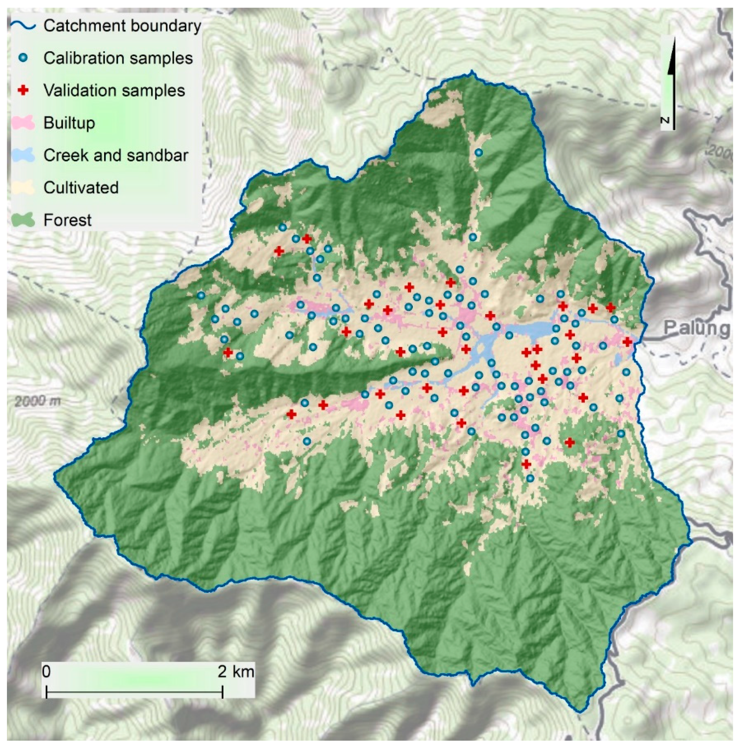
2.1. Study Area

The study was conducted in the Palung catchment, which is an upstream catchment of the Kulekhani watershed and lies in the middle mountain region of central Nepal (Figure 1). Extending across 27°35′41.4″ to 27°39′37.9″ north latitude and 85°1′20.3″ to 85°5′45.1″ east longitude over an area of 3076.7 ha, the elevation of the study area ranges from 1753 to 2605 m above the mean sea level. The boundary of the catchment was delineated using AW3D-5m DEM derived from the Advanced Land Observation Satellites of JAXA [21]. Influenced by the easy access to major urban centers, such as Kathmandu, this area is a pocket area for commercial vegetable production. The cropping pattern is similar across the arable lands in the catchment, and most soils are well drained. Vegetable production during the rainy season is a specialty of this area when most of the plain lands across the country are inundated with water.

Table 1. Local crop calendar of the study area.

Crop	Jan		Feb		Mar		Apr		May		Jun		Jul		Aug		Sep		Oct		Nov		Dec
Cauliflower
Cabbage
Radish
Chilli
Coriander
Potato
Maize
Symbols		Sowing/transplanting								Mid-season							Harvesting
Seasons	Winter				Pre-monsoon						Monsoon								Post-monsoon

shows the crop calendar of the major crops grown in this area and the classification of seasons that relate to the annual pattern of precipitation [22].

Upper and mostly steeper slopes of the catchment, which are less accessible and less amenable to cultivation, are covered by mixed forests. Regarding the climate, winter in this area is cold and frosty with mild summer temperatures, which is a typical characteristic of the higher ranges of the middle mountain physiographic region of Nepal. According to the meteorological data recorded by the nearest station of the Department of Hydrology and Meteorology at Daman, over the decade of the 2000s, the average annual precipitation received by this region was 1883 mm. The average annual maximum and minimum temperatures were 19.64 and 8.34 °C, respectively [23]. Soils were predominantly Glayic Cambisols with well drained sandy loam texture developed from colluvial deposits [24]. The predictive mapping of SOC in this study was confined to the cultivated lands of this catchment, which occupied 901.7 ha of the catchment.

2.2. Land Cover Mapping

The land cover map of the study area was derived from a Sentinel-2 image captured in October 2019. The level 2A surface reflectance image product was used as it was available and already atmospherically corrected. The object-based image analysis approach was followed to classify the image. Image segmentation and classification were carried out using the “Example-based classification approach” on ENVI 5.5 software [25]. The support vector machine algorithm was chosen to classify the image. Training samples were selected through visual interpretation of the image. Bands 2 (blue), 3 (green), 4 (red), and 8 (near-infrared), and four other spectral layers, namely normalized difference vegetation index (NDVI), hue, saturation, and value were used for the segmentation of the image. The mean and standard deviation of these bands, layers, and Haralick texture features were calculated from these bands and layers and were used for classifying the image segments. Validation was performed using the point locations collected during the fieldwork. Overall accuracy and Kappa statistics were calculated to evaluate the quality of classification output.

2.3. Soil Sampling and Laboratory Analysis

Two sets of SOC point data were collected from the field using a soil sampling auger. For calibrating the models, the conditioned Latin Hypercube (cLHS) sampling technique was used [26] and for validating the models, simple random sampling was adopted. The cLHS sampling design is an efficient model-based sampling strategy that is appropriate for efficient mapping of the spatial variability of soil properties [27] as it captures a maximum amount of variability in the covariate feature space with minimum possible sample points [26]. The terrain and Sentinel-2 based covariates were used as the covariates to allocate the sample locations across the feature space, and two raster surfaces, namely slope and distance to the roads were used to create the cost surface as an input to the cLHS model to assure the accessibility to the target sample point locations and to minimize the travel time needed to collect samples from across the catchment. Altogether, 114 topsoil (0–20 cm) samples were collected to calibrate the model, and 38 additional samples collected following probability sampling design were used to validate the model. Validating the prediction model using samp1es derived from probability sampling has been suggested as the superior method in comparison to other methods, such as data-splitting and cross-validation [28]. For a specific sample location, three soil samples were collected within a buffer distance of 1 m from the targeted sample points and composited into one. A handheld Garmin GPS device was used to navigate to the target sample points and record the geographic location of the samples collected in the field. The horizontal accuracy of the device was 3 m, and the allowed buffer distance of 1 m added up to 4 m. We aimed to make sure that the point soil sample was collected within a 5 m radius from the center of the selected pixels of the Sentinel-2 image. This way, the sample fell within the area of the image pixel, which was of 10 m spatial resolution. This minimizes the chance of the sampling point falling into the pixels surrounding the target pixels. Figure 2 shows the spatial distribution of calibration and validation datasets overlaid on the land cover map of the catchment.

Soil samples were analyzed in the laboratory of the Soil Science Division of Nepal Agricultural Research Council for soil organic matter determination using the Walkley-Black wet oxidation method [29]. A correction factor of 1.3 was used to account for partial oxidation of organic matter [30]. After that, the organic matter content of the soil samples was multiplied by the van Bemmelen conversion coefficient of 0.58 to obtain SOC percent values [31]. The SOC concentration in percent was then multiplied by 10 to convert it to g kg⁻¹.

2.4. Covariates

The environmental covariates were collected from two major sources. The terrain-based covariates were derived using AW3D-5m DEM, derived from the Advanced Land Observation Satellites of JAXA [21] that was resampled to 10 m to align it with the origin resolution of the Sentinel-2 images [21] using the SAGA-GIS software platform [32]. Remote sensing-based covariates were based on the Sentinel-2 images obtained in three different months, namely February, May, and November, representing three different seasons in the local crop calendar. The Sentinel-2 image bands included in this study to construct the covariates were Band 2 (blue), Band 3 (green), Band 4 (red), Band 5 (red edge), Band 8 (near-infrared), Band 8A (narrow-infrared), Band 11, and 12 (shortwave-infrared (SWIR)).

The K-T components were calculated in the Google Earth Engine (GEE) platform using the coefficients for the six-band model advised by Shi and Xu [33]. In addition, the Sentinel-2 Leaf Area Index (SeLI) was calculated using the red-edge (band 5) and the narrow near-infrared (Band 8a) bands [34]. These two bands were not used while generating K-T transformed indices. Details on the covariates used to construct different prediction models are presented in

Table 2. Covariates used to build predictive models.

Covariate	Description	Reference
Remote sensing-based
bright_feb	K-T transformed brightness component for an at-sensor Sentinel-2 median image of February 2020	[19,33]
green_feb	K-T transformed greenness component for an at-sensor Sentinel-2 median image of February 2020	[19,33]
Wet_feb	K-T transformed wetness component for an at-sensor Sentinel-2 median image of February 2020	[19,33]
SeLI_feb	Sentinel-2 LAI Index for February 2020	[34]
bright_may	K-T transformed brightness component for an at-sensor Sentinel-2 median image of May 2020	[19,33]
green_may	K-T transformed greenness component for an at-sensor Sentinel-2 median image of May 2020	[19,33]
Wet_may	K-T transformed wetness component for an at-sensor Sentinel-2 median image of May 2020	[19,33]
SeLI_may	Sentinel-2 LAI Index for May 2020	[34]
bright_nov	K-T transformed brightness component for an at-sensor Sentinel-2 median image of November 2019	[19,33]
green_nov	K-T transformed greenness component for an at-sensor Sentinel-2 median image of November 2019	[19,33]
Wet_nov	K-T transformed wetness component for an at-sensor Sentinel-2 median image of November 2019	[19,33]
SeLI_nov	Sentinel-2 LAI Index for November 2019	[34]
Terrain based
elevation	Elevation (meters above sea level)	[21]
maxElDev	Maximum elevation deviation	[35]
mid_slope	Mid-slope position	[32]
ls_factor	Slope length and steepness factor	[32]
curv_plan	Plan curvature	[32]
insolation	Direct annual solar radiation	[36]
twi	Topographic wetness index (SAGA)	[32]
mrrtf	Multi-resolution index of ridge-top flatness	[32]
mTPI	Multiscale topographic position index	[32]

. The Median monthly image composites were created by taking the median pixel values from the time-series of images obtained within a given month. The median pixel values were used to avoid the influence of outliers that might have been introduced due to bad pixel values or atmospheric anomalies during image acquisition. Sentinel-2 Level 1A products were used for this study, which were available as both geometrically and atmospherically corrected values.

2.5. Prediction Models

Nine random forest (RF) models [37] were built using nine sets of covariates representing different combinations of terrain covariates and Sentinel-2-based covariates for three different seasons/months, as listed below. A local cropping calendar was used to match the seasons/months of the images. RF models were used because their predictive performance was reported to be superior in the majority of the recent SOC mapping and modeling studies in a systematic review [38,39,40]. The RF models are trained to create ensemble estimates from a set of regression trees built from bootstrap samples. The final predictions of the target attributes are the averages of the predictions of individual regression trees [37,41]. The models constructed to predict SOC contents are listed below.

• Model 1. Sentinel-2 (Feb)
• Model 2. Sentinel-2 (May)
• Model 3. Sentinel-2 (Nov)
• Model 4. Sentinel-2 (Feb, May, Nov)
• Model 5. Terrain only
• Model 6. Terrain + Sentinel-2 (Feb)
• Model 7. Terrain + Sentinel-2 (May)
• Model 8. Terrain + Sentinel-2 (Nov)
• Model 9. All (Terrain + Sentinel-2 (Feb, May, Nov))

2.6. Model Evaluation and Uncertainty

2.6.1. Evaluation of Prediction

External validation was performed to test the results of the predictive models on 38 samples collected through probability sampling. Mean error (ME), root mean square error (RMSE), and R² were computed to compare model performance. In order to assess which models predicted better for the calibration sites, these indices were also calculated for calibration datasets.

$${\mathrm{R}}^2=\frac{{{\displaystyle \sum }}_{\mathrm{i}=1}^{\mathrm{n}}{\left({\mathrm{predicted}}_{\mathrm{i}}-\overline{\mathrm{observed}}\right)}^2}{{{\displaystyle \sum }}_{\mathrm{i}=1}^{\mathrm{n}}{\left({\mathrm{observed}}_{\mathrm{i}}-\overline{\mathrm{observed}}\right)}^2}$$

(1)

$$\mathrm{RMSE}=\sqrt{\frac{1}{\mathrm{n}}{\displaystyle \sum }_{\mathrm{i}=1}^{\mathrm{n}}{\left({\mathrm{observed}}_{\mathrm{i}}-{\mathrm{predicted}}_{\mathrm{i}}\right)}^2}$$

(2)

$$\mathrm{ME}=\frac{1}{\mathrm{n}}{\displaystyle \sum }_{\mathrm{i}=1}^{\mathrm{n}}\left({\mathrm{observed}}_{\mathrm{i}}-{\mathrm{predicted}}_{\mathrm{i}}\right)$$

(3)

2.6.2. Measure of Prediction Uncertainty

The quantile regression forest (QRF) approach was used to analyze the model’s uncertainty in a spatially explicit manner [42,43,44]. The model uncertainty was estimated as a function of the specified prediction variables as represented by the full conditional distribution of the response variable (SOC in our case) using the QRF technique in the ‘quantregForest’ package on the R software platform [45,46]. This technique computed a probability distribution function for each pixel, and the standard deviation calculated from the entire prediction range was divided by the mean SOC prediction and expressed in percentage for an easier interpretation of the model uncertainty [47].

3. Results

3.1. Land Cover Map

Figure 2 shows the land cover map produced using a Sentinel-2 image from which four major land cover categories were extracted, namely, cultivated lands (area 901.7 ha), forests (2056.5 ha), built-up areas (88.7 ha), and creeks, including adjacent sandbars (29.8 ha). As calculated using a DEM of 10 m resolution, the mean slope of the cultivated areas was 16.35°, and that of the forest areas was 31.68°. Accuracy of the land cover classification was carried out using 182 point locations with an overall accuracy of 92.31% and a kappa coefficient of 0.87.

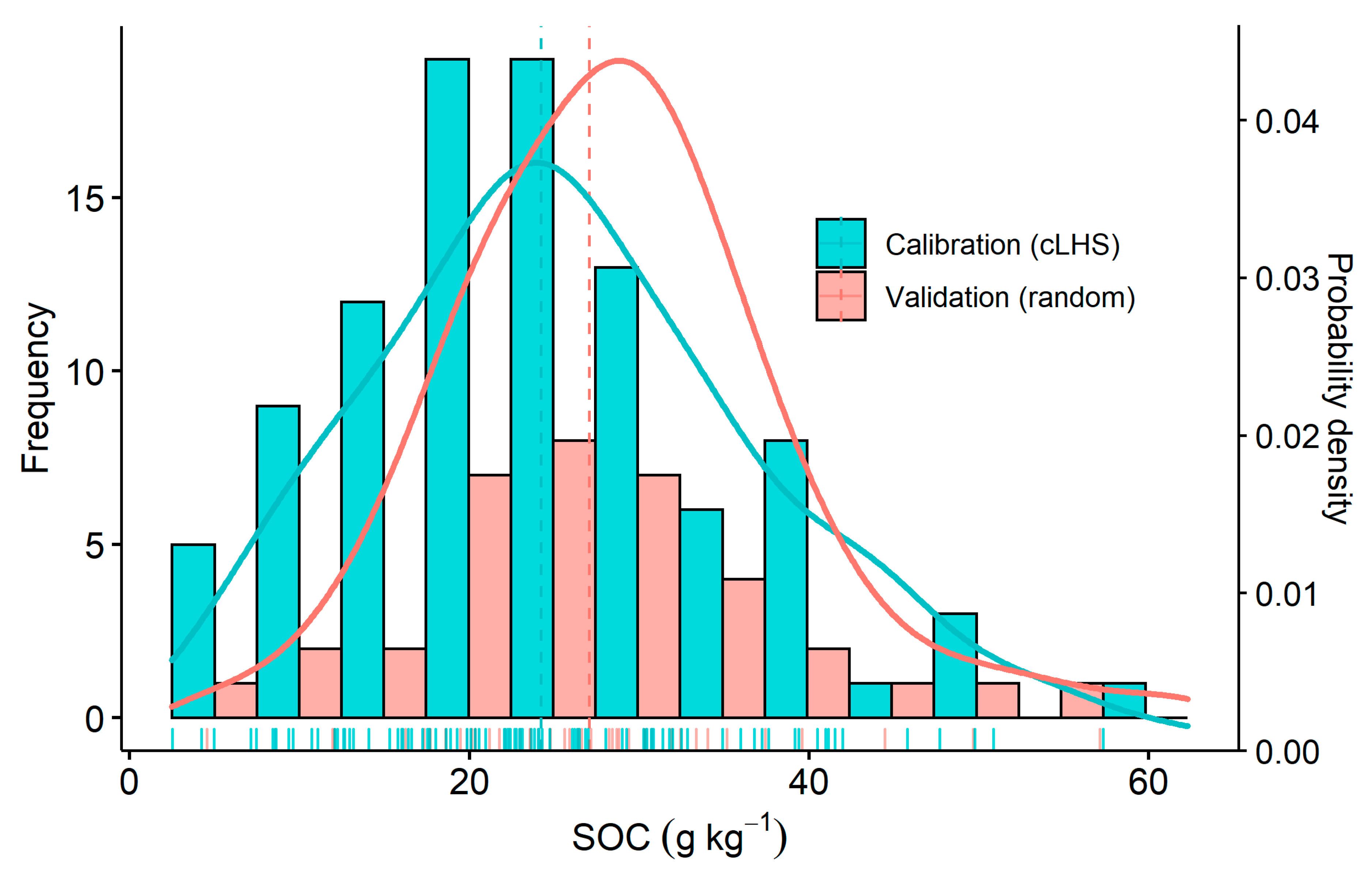
3.2. General Statistics

Descriptive statistics of SOC measurements on calibration and validation points are presented in

Table 3. Descriptive statistics of the soil organic carbon content (g kg⁻¹) in the calibration and validation datasets.

Statistics	Calibration	Validation	All
Number of samples (n)	114	38	152
Min (g kg−1)	2.50	4.54	2.50
Mean (g kg−1) ± 95% Confidence interval	24.21 ± 2.27	27.04 ± 3.52	24.98 ± 1.9
Median (g kg−1)	22.94	26.50	23.72
Max (g kg−1)	57.32	57.12	57.32
Standard deviation (g kg−1)	11.20	10.41	11.02
Standard error of the mean (g kg−1)	1.14	1.73	0.96
Skewness	0.49	0.62	0.5
Kurtosis	−0.02	0.84	0.22

. The measured SOC content ranged from 2.5 to 57.3 g kg⁻¹ with a mean of 24.98 ± 1.9 g kg⁻¹. High variation in the SOC contents is due to the diversity in the terrain and the subsequent differences in microclimate and soil management within the study area.

Figure 3 illustrates the frequency distribution of the SOC contents in the calibration and validation datasets. Bars represent the histograms, and the curves show the probability density. The rug plots show the location of individual sample points along the continuum of SOC content values in the X-axis. The distribution of the values of the SOC content is somewhat bell-shaped, indicating that it is following a normal distribution. Transformations (log and square root) did not improve the distribution to make it more normal. Therefore, the original SOC values were used for fitting the predictive models. In addition, unlike the conventional regression models, the machine learning model used in this study did not require the data to be of normal distribution. To avoid the issues related to spatial autocorrelation, before fitting the predictive models to the observed data, a test of spatial autocorrelation was performed using the Global Moran’s I test [48,49]. The spatial pattern did not show significant spatial autocorrelation.

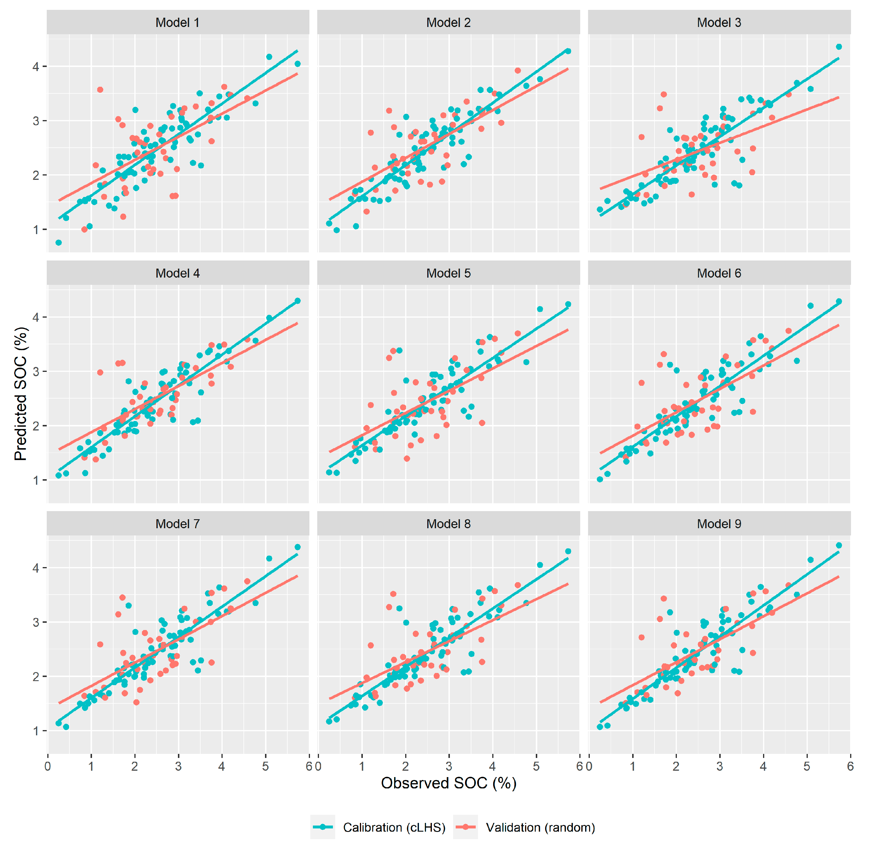
3.3. Evaluation of Prediction Models

The goodness of fit and error statistics of the predictive models used in this study are presented in

Table 4. Goodness of fit and error statistics of predictive models.

Prediction Models	R2		RMSE		MAE
	Cal	Val	Cal	Val	Cal	Val
Model1 [Sentinel-2 (Feb)]	0.69	0.35	2.81	5.31	2.17	4.10
Model 2 [Sentinel-2 (May)]	0.67	0.31	2.99	5.64	2.24	4.23
Model 3 [Sentinel-2 (Nov)]	0.64	0.22	3.05	5.75	2.26	4.27
Model 4 [Sentinel-2 (Feb, May, Nov)]	0.76	0.42	2.73	5.16	2.12	4.00
Model 5 [Terrain only]	0.68	0.35	2.84	5.35	2.22	4.19
Model 6 [Terrain + Sentinel-2 (Feb)]	0.79	0.45	2.67	5.04	2.08	3.93
Model 7 [Terrain + Sentinel-2 (May)]	0.73	0.40	2.72	5.13	2.13	4.02
Model 8 [Terrain + Sentinel-2 (Nov)]	0.71	0.37	2.90	5.47	2.17	4.10
Model 9 [All (Terrain + Sentinel-2 (Feb, May, Nov)]	0.81	0.46	2.16	4.08	2.07	3.91

Note: R²: coefficient of determination, RMSE: root mean squared error, MAE: mean absolute error

. The observed and predicted SOC contents for each of the nine models are shown in Figure 4. The model that used all-terrain variables and the Sentinel-2 images of all three cropping seasons yielded the best prediction results with the R²_cal 0.81 and the R²_val 0.46, followed closely by the one that used the Terrain variables and the Sentinel-2 image obtained in February, which had the R²_cal 0.79 and the R²_val 0.45. The RMSE and MAE were also in favor of these two models in comparison to other models. The model with only the Sentinel-2 image captured in November had the lowest predictive power for predicting SOC in the cultivated lands of this catchment.

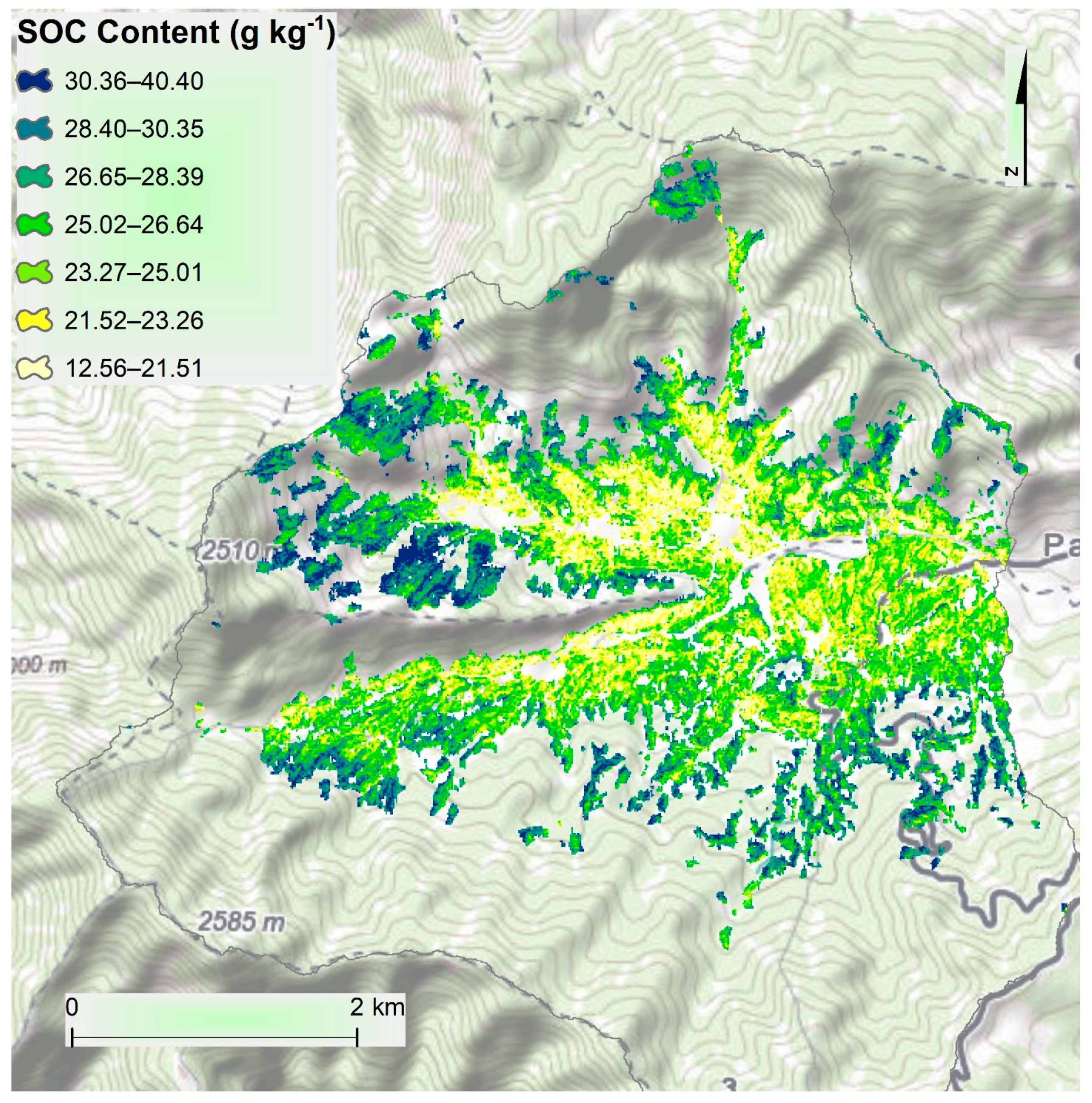
3.4. Spatial Distribution of SOC in the Catchment

Figure 5 shows the spatial distribution of the predicted topsoil SOC contents in the catchment based on the model that included all covariates as predictors, as this model performed better than other models. The predicted SOC content ranged from 12.5 to 40.4 g kg⁻¹, with a mean of 25.6 g kg⁻¹. The spatial pattern of the SOC contents shows that there was a higher level of SOC contents in the upstream areas of the catchment in comparison to the downstream areas.

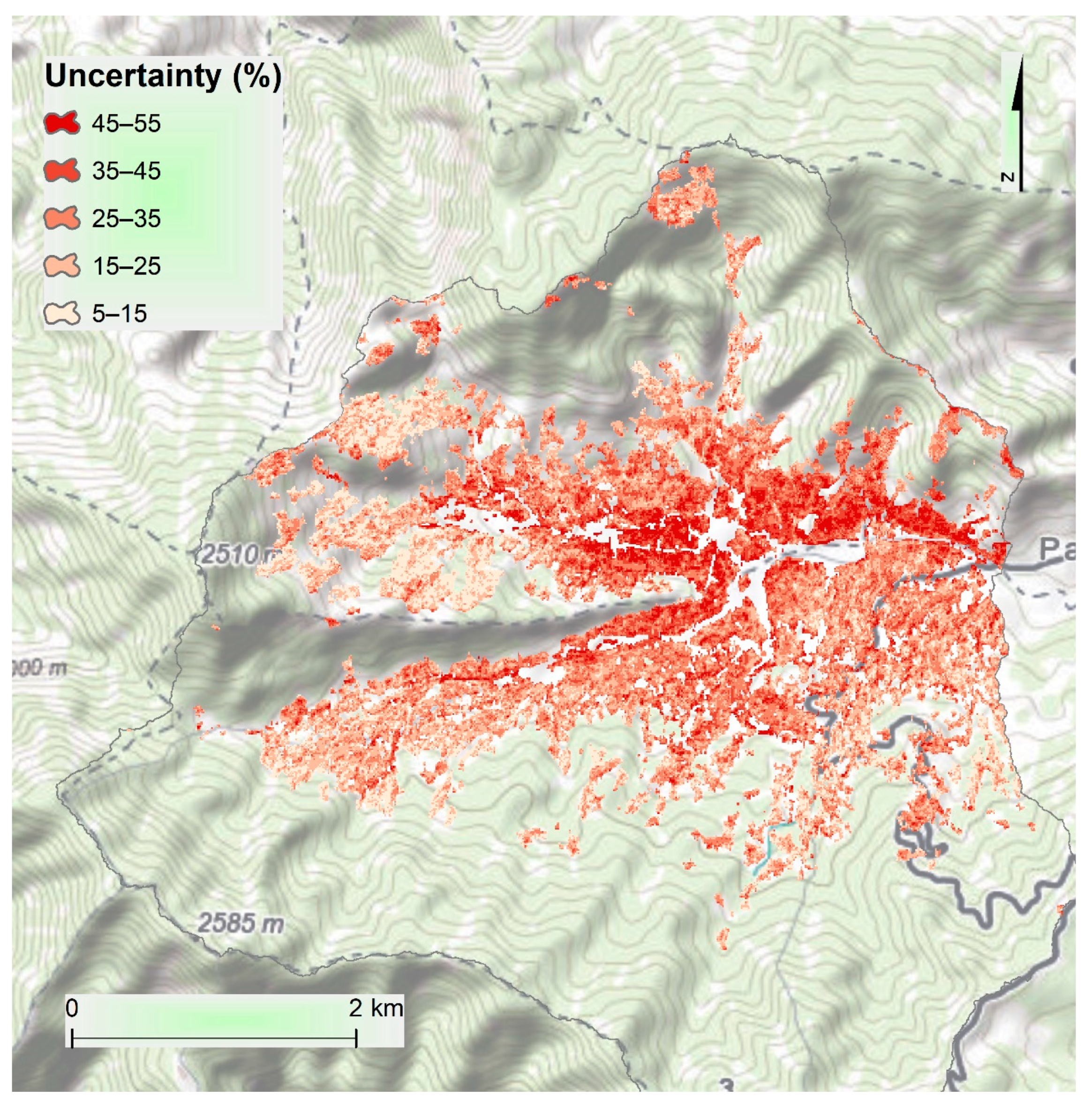
3.5. Uncertainty Assessment

The uncertainty map of the model prediction is presented in Figure 6; it was based on the model that performed the best among the nine different models. The prediction uncertainty ranged between 5 and 55%. The uncertainty shown here is the standard deviation of prediction expressed as the percentage of the mean prediction of topsoil SOC contents. Less uncertainty indicates that the prediction was more precise in those areas when the model was used for prediction. The spatial pattern of the uncertainty map shows that the lower and flatter areas of the catchment had higher uncertainty compared to the upper areas of the catchment.

3.6. Variable Importance

The importance of variables in all nine prediction models used in this study is presented in Figure 7. When only the Sentinel-2 images of a single season were used, the brightness index was the most important predictor in February and November (Figure 7a,c) and the greenness index in May (Figure 7b). When the Sentinel-2 images from all three cropping seasons were used together, the SeLI of February was rated as the most influential variable, followed by the greenness index of May and the brightness index of November (Figure 7d). In the model that used only the terrain variables, elevation was the most influential covariate, followed by the maximum elevation deviation and mid-slope position (Figure 7e). The brightness index, elevation, and SeLI were the most important covariates in the model that used terrain variables and the Sentinel-2 image indices from February (Figure 7f). In the model that used terrain variables plus Sentinel-2 image indices from May, elevation, maximum elevation deviation, and the mid-slope position index were ranked as the most important variables (Figure 7g). The model using the terrain variables and the Sentinel-2 image indices from November ranked elevation, maximum elevation deviation, and wetness index as the most influential variables (Figure 7h). The model that used all covariates, including the terrain variables and the Sentinel-2 image indices from all three cropping seasons, ranked elevation, SeLI (February), mid-slope position, maximum elevation deviation, and the brightness index (November), as the most influential variables (Figure 7i).

4. Discussion

An object-based image analysis approach with the SVM algorithm was found to be effective at classifying a Sentinel-2 satellite image to extract major land cover types. Most of the cultivated lands were situated at the downstream areas of the catchment. Downstream areas were flatter than the upstream areas of the catchment, rendering the downstream areas more amenable to tillage operations. However, it was also not uncommon to cultivate upstream areas of the catchment where bench terraces were built on the steep slopes.

The prediction model that used all covariates performed better than the other models. When comparing only the Sentinel-2-based covariates from three different seasons/months, those of February performed better than those from May and November. In February, the cultivated lands in this catchment are fallow with the least vegetation cover, and the bare soil surface is exposed. The reflectance obtained during this season is mostly from the bare soils, and the predictive capacity of the satellite images can be expected to be higher than the images obtained during other seasons when the land is covered with vegetation [5]. The model that used only the Sentinel-2 image covariates obtained in November had the lowest performance. The terrain-only model performed similarly to that obtained using the Sentinel-2 February model. The performance of the model that used the terrain variables and Sentinel-2-based covariates obtained in February performed very similarly to the all-covariate model. In this mountainous region, topography controls the micro-climatic variation, soil erosion, and deposition processes. As a consequence, SOC can be expected to be influenced by the features of the landform. A model that uses all covariates might predict better than partial models. However, there might be a risk of overfitting models to the specific datasets. Therefore, the model that used terrain features and Sentinel-2 image-based covariates obtained from February (Model 6) can be recommended as an optimum one, which performed very close to the all-covariate model (Model 9).

Downstream areas are more intensively cultivated than the upstream counterparts of this catchment. In addition, the soil surface temperature in the upper elevation is lower than that in the lower elevations. The intensive tillage operations are expected to expose soils to the atmosphere, and higher temperatures accelerate the process of the oxidation of organic carbon and release it into the atmosphere [50]. Decomposition processes are aided further by the combination of warm and moist soil conditions that promote microbial activity [51]. This resulted in lower levels of SOC contents in the lower regions of the catchment. Conversely, upland areas are tilled less frequently. Accompanied by the lower temperatures, these upper regions are expected to experience reduced loss of SOC from the soils.

Cultivated lands of the downstream areas appear to have a higher level of uncertainty in comparison to upstream areas of the catchment. This can be explained by the variability in the management practices of the cultivated lands, which are more intensively cultivated [52]. The management factors that might have influenced the spatial variability in the levels of SOC contents in these downstream cultivated areas may not have been captured by the covariates used in these predictive models. The steep upstream areas are less intensively cultivated, which may have less influence due to the management and because they are more strongly controlled by the terrain features.

Regarding the importance of covariates, the brightness index was picked as the most influential variable by the models that used the Sentinel-2 image-based covariates of individual months or seasons. It has been reported that SOC increases the darkness of the soils, hence the reverse correlation of SOC contents with the brightness index [53]. SeLI was another important covariate based on the Sentinel-2 satellite image. SeLI index was constructed using the red-edge band, and the narrow-infrared band was ranked among the high impact covariate by the all-Sentinel-2 model and all-covariates model. Studies have reported that SOC is sensitive to the bands in these spectral regions. Among the terrain variables, elevation was consistently the most influential covariate [8,54,55]. Maximum elevation deviation and the mid-slope position were also ranked as highly influential terrain covariates by these prediction models. The elevation is directly correlated with the soil surface temperature in general and indirectly with the intensity of management or cultivation practices, specifically in this catchment [56]. The soil surface temperature and management factors are reported to be important variables that determine the spatial variability in the level of SOC. The maximum elevation deviation shows the variation of terrain relief, which is likely to influence the local climatic condition and, therefore, the level of SOC contents. The mid-slope position index measures the position in a sloping landscape along the slope of the terrain. It indicates the difference in the air temperature along the vertical span of slopes. In general, the middle sections of the terrain slope are warmer than the upper and lower ends [57]. This difference in air temperature near the surface of the earth can influence the level of SOC loss from the soils. Therefore, these terrain covariates are relevant in determining the levels of SOC contents in this catchment.

5. Conclusions

This study evaluated the performance of terrain variables and Sentinel-2 image-based indices from three different cropping seasons for the predictive mapping of SOC. Calibration soil sample points were collected using a cLHS approach, and validation samples were selected using an additional probability sampling approach. The model that used terrain and image-based indices from all seasons (Model 9) had the greatest predictive performance. However, the model with the terrain variables and the image-based indices from February (Model 6) were very close to the predictive performance of the full model (Model 9) that used all covariates. In order to capture the maximum possible variability in SOC contents, a mix of relevant terrain and multi-season remote sensing-based covariates are recommended. Among them, elevation, maximum elevation deviation, and mid-slope position are the most important terrain covariates, and brightness index and SeLI are the most influential remote sensing-based covariates for the predictive mapping of SOC contents. Therefore, it can be concluded that the terrain variables and the multi-season Sentinel-2 image indices obtained in different seasons of a local cropping calendar can improve the prediction of SOC. Furthermore, the combination of terrain variables and the Sentinel-2 image from February can also make an optimal and parsimonious prediction model for the improved digital mapping of SOC in the catchments similar to this study area. However, it should be remembered that the month of imagery will depend on the local cropping pattern.

References

1. Drewniak, B.; Mishra, U.; Song, J.; Prell, J.; Kotamarthi, V. Modeling the impact of agricultural land use and management on US carbon budgets. Biogeosciences 2015, 12, 2119–2129. [Google Scholar] [CrossRef] [Green Version]
2. Ren, W.; Banger, K.; Tao, B.; Yang, J.; Huang, Y.; Tian, H. Global pattern and change of cropland soil organic carbon during 1901–2010: Roles of climate, atmospheric chemistry, land use and management. Geogr. Sustain. 2020, 1, 59–69. [Google Scholar] [CrossRef]
3. McHunu, C.; Chaplot, V. Land degradation impact on soil carbon losses through water erosion and CO2 emissions. Geoderma 2012, 177–178, 72–79. [Google Scholar] [CrossRef]
4. de Gruijter, J.J.; McBratney, A.B.; Minasny, B.; Wheeler, I.; Malone, B.P.; Stockmann, U. Farm-scale soil carbon auditing. Geoderma 2016, 265, 120–130. [Google Scholar] [CrossRef]
5. Vaudour, E.; Gomez, C.; Lagacherie, P.; Loiseau, T.; Baghdadi, N.; Urbina-Salazar, D.; Loubet, B.; Arrouays, D. Temporal mosaicking approaches of Sentinel-2 images for extending topsoil organic carbon content mapping in croplands. Int. J. Appl. Earth Obs. Geoinf. 2021, 96, 102277. [Google Scholar] [CrossRef]
6. Zhou, T.; Geng, Y.; Ji, C.; Xu, X.; Wang, H.; Pan, J.; Bumberger, J.; Haase, D.; Lausch, A. Prediction of soil organic carbon and the C:N ratio on a national scale using machine learning and satellite data: A comparison between Sentinel-2, Sentinel-3 and Landsat-8 images. Sci. Total Environ. 2021, 755, 142661. [Google Scholar] [CrossRef] [PubMed]
7. Vaudour, E.; Gomez, C.; Loiseau, T.; Baghdadi, N.; Loubet, B.; Arrouays, D.; Ali, L.; Lagacherie, P. The Impact of Acquisition Date on the Prediction Performance of Topsoil Organic Carbon from Sentinel-2 for Croplands. Remote Sens. 2019, 11, 2143. [Google Scholar] [CrossRef] [Green Version]
8. Fathololoumi, S.; Vaezi, A.R.; Alavipanah, S.K.; Ghorbani, A.; Saurette, D.; Biswas, A. Improved digital soil mapping with multitemporal remotely sensed satellite data fusion: A case study in Iran. Sci. Total Environ. 2020, 721, 137703. [Google Scholar] [CrossRef]
9. McBratney, A.B.; Mendonça Santos, M.L.; Minasny, B. On digital soil mapping. Geoderma 2003, 117, 3–52. [Google Scholar] [CrossRef]
10. Rawlins, B.G.; Marchant, B.P.; Smyth, D.; Scheib, C.; Lark, R.M.; Jordan, C. Airborne radiometric survey data and a DTM as covariates for regional scale mapping of soil organic carbon across Northern Ireland. Eur. J. Soil Sci. 2009, 60, 44–54. [Google Scholar] [CrossRef] [Green Version]
11. Taghizadeh-Mehrjardi, R.; Nabiollahi, K.; Kerry, R. Digital mapping of soil organic carbon at multiple depths using different data mining techniques in Baneh region, Iran. Geoderma 2016, 266, 98–110. [Google Scholar] [CrossRef]
12. Peng, Y.; Xiong, X.; Adhikari, K.; Knadel, M.; Grunwald, S.; Greve, M.H. Modeling soil organic carbon at regional scale by combining multi-spectral images with laboratory spectra. PLoS ONE 2015, 10, e0142295. [Google Scholar] [CrossRef] [Green Version]
13. Angelopoulou, T.; Tziolas, N.; Balafoutis, A.; Zalidis, G.; Bochtis, D. Remote Sensing Techniques for Soil Organic Carbon Estimation: A Review. Remote Sens. 2019, 11, 676. [Google Scholar] [CrossRef] [Green Version]
14. Castaldi, F.; Hueni, A.; Chabrillat, S.; Ward, K.; Buttafuoco, G.; Bomans, B.; Vreys, K.; Brell, M.; van Wesemael, B. Evaluating the capability of the Sentinel 2 data for soil organic carbon prediction in croplands. ISPRS J. Photogramm. Remote Sens. 2019, 147, 267–282. [Google Scholar] [CrossRef]
15. Gholizadeh, A.; Žižala, D.; Saberioon, M.; Borůvka, L. Soil organic carbon and texture retrieving and mapping using proximal, airborne and Sentinel-2 spectral imaging. Remote Sens. Environ. 2018, 218, 89–103. [Google Scholar] [CrossRef]
16. Li, X.; Ding, J.; Liu, J.; Ge, X.; Zhang, J. Digital Mapping of Soil Organic Carbon Using Sentinel Series Data: A Case Study of the Ebinur Lake Watershed in Xinjiang. Remote Sens. 2021, 13, 769. [Google Scholar] [CrossRef]
17. Dou, X.; Wang, X.; Liu, H.; Zhang, X.; Meng, L.; Pan, Y.; Yu, Z.; Cui, Y. Prediction of soil organic matter using multi-temporal satellite images in the Songnen Plain, China. Geoderma 2019, 356, 113896. [Google Scholar] [CrossRef]
18. Hill, J.; Schütt, B. Mapping Complex Patterns of Erosion and Stability in Dry Mediterranean Ecosystems. Remote Sens. Environ. 2000, 74, 557–569. [Google Scholar] [CrossRef]
19. Kauth, R.J.; Thomas, G. The tasselled cap—A graphic description of the spectral-temporal development of agricultural crops as seen by Landsat. In Proceedings of the LARS Symposia, West Lafayette, IN, USA, 29 June–1 July 1976; p. 159. [Google Scholar]
20. ESRI. Tasseled Cap Function. Available online: https://pro.arcgis.com/en/pro-app/latest/help/analysis/raster-functions/tasseled-cap-function.htm (accessed on 30 June 2021).
21. Tadono, T.; Takaku, J.; Tsutsui, K.; Oda, F.; Nagai, H. Status of “ALOS World 3D (AW3D)” global DSM generation. In Proceedings of the 2015 IEEE International Geoscience and Remote Sensing Symposium (IGARSS), Milan, Italy, 26–31 July 2015; pp. 3822–3825. [Google Scholar]
22. Talchabhadel, R.; Karki, R.; Thapa, B.R.; Maharjan, M.; Parajuli, B. Spatio-temporal variability of extreme precipitation in Nepal. Int. J. Climatol. 2018, 38, 4296–4313. [Google Scholar] [CrossRef]
23. NARC/AFACI. 3rd Annual Technical Report on Agro-Meteorological Information for the Adaptation to Climate Change in Nepal; NARC/AFACI—AMIS Project: Khumaltar, Lalitpur, Nepal, 2015. [Google Scholar]
24. Lamichhane, S.; Kumar, L.; Adhikari, K. Updating the national soil map of Nepal through digital soil mapping. Geoderma 2021, 394, 115041. [Google Scholar] [CrossRef]
25. Exelis Visual Information Solutions; ENVI, 5.5; L3 Harris Geospatial: Boulder, CO, USA, 2019.
26. Minasny, B.; McBratney, A.B. A conditioned Latin hypercube method for sampling in the presence of ancillary information. Comput. Geosci. 2006, 32, 1378–1388. [Google Scholar] [CrossRef]
27. Brus, D. Design-based and model-based sampling strategies for soil monitoring. In Proceedings of the 19th World Congress of Soil Science, Solutions for a Changing World, Brisbane, Australia, 1–6 August 2010. [Google Scholar]
28. Brus, D.J.; Kempen, B.; Heuvelink, G.B.M. Sampling for validation of digital soil maps. Eur. J. Soil Sci. 2011, 62, 394–407. [Google Scholar] [CrossRef]
29. Walkley, A.J.; Black, I.A. Estimation of soil organic carbon by the chromic acid titration method. Soil Sci. 1934, 37, 29–38. [Google Scholar] [CrossRef]
30. Nelson, D.W.; Sommers, L.E. Total Carbon, Organic Carbon, and Organic Matter. In Methods of Soil Analysis Part 3—Chemical Methods; Sparks, D.L., Page, A.L., Helmke, P.A., Loeppert, R.H., Eds.; SSSA Book Series; Soil Science Society of America, American Society of Agronomy: Madison, WI, USA, 1996; pp. 961–1010. [Google Scholar]
31. Van Bemmelen, J. Über die Bestimmung des Wassers, des Humus, des Schwefels, der in den colloïdalen Silikaten gebundenen Kieselsäure, des Mangans usw im Ackerboden. Die Landwirthschaftlichen Versuchs-Stationen 1890, 37, e290. [Google Scholar]
32. Conrad, O.; Bechtel, B.; Bock, M.; Dietrich, H.; Fischer, E.; Gerlitz, L.; Wehberg, J.; Wichmann, V.; Böhner, J. System for automated geoscientific analyses (SAGA) v. 2.1. 4. Geosci. Model Dev. Discuss. 2015, 8, 1991–2007. [Google Scholar] [CrossRef] [Green Version]
33. Shi, T.; Xu, H. Derivation of Tasseled Cap Transformation Coefficients for Sentinel-2 MSI At-Sensor Reflectance Data. IEEE J. Sel. Top. Appl. Earth Obs. Remote Sens. 2019, 12, 4038–4048. [Google Scholar] [CrossRef]
34. Pasqualotto, N.; Delegido, J.; Van Wittenberghe, S.; Rinaldi, M.; Moreno, J. Multi-crop green LAI estimation with a new simple Sentinel-2 LAI Index (SeLI). Sensors 2019, 19, 904. [Google Scholar] [CrossRef] [PubMed] [Green Version]
35. Lindsay, J.B. WhiteboxTools User Manual; Geomorphometry and Hydrogeomatics Research Group, University of Guelph: Guelph, ON, Canada, 2018. [Google Scholar]
36. Kumar, L.; Skidmore, A.K.; Knowles, E. Modelling topographic variation in solar radiation in a GIS environment. Int. J. Geogr. Inf. Sci. 1997, 11, 475–497. [Google Scholar] [CrossRef]
37. Breiman, L. Random Forests. Mach. Learn. 2001, 45, 5–32. [Google Scholar] [CrossRef] [Green Version]
38. Lamichhane, S.; Kumar, L.; Wilson, B. Digital soil mapping algorithms and covariates for soil organic carbon mapping and their implications: A review. Geoderma 2019, 352, 395–413. [Google Scholar] [CrossRef]
39. Forkuor, G.; Hounkpatin, O.K.L.; Welp, G.; Thiel, M. High resolution mapping of soil properties using Remote Sensing variables in south-western Burkina Faso: A comparison of machine learning and multiple linear regression models. PLoS ONE 2017, 12, e0170478. [Google Scholar] [CrossRef]
40. Zeraatpisheh, M.; Ayoubi, S.; Jafari, A.; Tajik, S.; Finke, P. Digital mapping of soil properties using multiple machine learning in a semi-arid region, central Iran. Geoderma 2019, 338, 445–452. [Google Scholar] [CrossRef]
41. Hengl, T.; Nussbaum, M.; Wright, M.N.; Heuvelink, G.B.M.; Gräler, B. Random forest as a generic framework for predictive modeling of spatial and spatio-temporal variables. PeerJ 2018, 6, e5518. [Google Scholar] [CrossRef] [PubMed] [Green Version]
42. Meinshausen, N. Quantile regression forests. J. Mach. Learn. Res. 2006, 7, 983–999. [Google Scholar]
43. Vaysse, K.; Lagacherie, P. Using quantile regression forest to estimate uncertainty of digital soil mapping products. Geoderma 2017, 291, 55–64. [Google Scholar] [CrossRef]
44. Dharumarajan, S.; Kalaiselvi, B.; Suputhra, A.; Lalitha, M.; Vasundhara, R.; Kumar, K.S.A.; Nair, K.M.; Hegde, R.; Singh, S.K.; Lagacherie, P. Digital soil mapping of soil organic carbon stocks in Western Ghats, South India. Geoderma Reg. 2021, 25, e00387. [Google Scholar] [CrossRef]
45. Meinshausen, N. Quantregforest: Quantile Regression Forests; R Package Version 1.3-7; Zurich, Switzerland, 2017; Available online: https://cran.r-project.org/web/packages/quantregForest/index.html (accessed on 6 September 2021).
46. R Core Team. R: A Language and Environment for Statistical Computing; The R Foundation for Statistical Computing: Vienna, Austria, 2020. [Google Scholar]
47. Yigini, Y.; Olmedo, G.F.; Reiter, S.; Baritz, R.; Viatkin, K.; Vargas, R. (Eds.) Soil Organic Carbon Mapping Cookbook, 2nd ed.; FAO: Rome, Italy, 2018; p. 220. [Google Scholar]
48. Ploton, P.; Mortier, F.; Réjou-Méchain, M.; Barbier, N.; Picard, N.; Rossi, V.; Dormann, C.; Cornu, G.; Viennois, G.; Bayol, N.; et al. Spatial validation reveals poor predictive performance of large-scale ecological mapping models. Nat. Commun. 2020, 11, 4540. [Google Scholar] [CrossRef]
49. Moran, P.A. Notes on continuous stochastic phenomena. Biometrika 1950, 37, 17–23. [Google Scholar] [CrossRef]
50. Ghimire, R.; Lamichhane, S.; Acharya, B.S.; Bista, P.; Sainju, U.M. Tillage, crop residue, and nutrient management effects on soil organic carbon in rice-based cropping systems: A review. J. Integr. Agric. 2017, 16, 1–15. [Google Scholar] [CrossRef]
51. Baldock, J.A. Composition and Cycling of Organic Carbon in Soil. In Nutrient Cycling in Terrestrial Ecosystems; Marschner, P., Rengel, Z., Eds.; Springer: Berlin/Heidelberg, Germany, 2007; pp. 1–35. [Google Scholar]
52. Wang, Y.; Wang, S.; Adhikari, K.; Wang, Q.; Sui, Y.; Xin, G. Effect of cultivation history on soil organic carbon status of arable land in northeastern China. Geoderma 2019, 342, 55–64. [Google Scholar] [CrossRef]
53. Mandal, U. Spectral color indices based geospatial modeling of soil organic matter in Chitwan district, Nepal. ISPRS—Int. Arch. Photogramm. Remote Sens. Spat. Inf. Sci. 2016, XLI-B2, 43–48. [Google Scholar] [CrossRef] [Green Version]
54. Hengl, T.; Heuvelink, G.B.M.; Kempen, B.; Leenaars, J.G.B.; Walsh, M.G.; Shepherd, K.D.; Sila, A.; MacMillan, R.A.; De Jesus, J.M.; Tamene, L.; et al. Mapping soil properties of Africa at 250 m resolution: Random forests significantly improve current predictions. PLoS ONE 2015, 10, e0125814. [Google Scholar] [CrossRef]
55. Vaysse, K.; Lagacherie, P. Evaluating Digital Soil Mapping approaches for mapping GlobalSoilMap soil properties from legacy data in Languedoc-Roussillon (France). Geoderma Reg. 2015, 4, 20–30. [Google Scholar] [CrossRef]
56. Nayava, J.L. Estimation of Temperature over Nepal. Himal. Rev. 1982, 14, 12–24. [Google Scholar]
57. Geiger, R.; Aron, R.H.; Todhunter, P. The Climate near the Ground, 5th ed.; Vieweg: Braunschweig, Germany, 1995. [Google Scholar]
Figure 1. Location of the study area.
Remotesensing 13 04772 g001
Figure 2. Distribution of the calibration and validation datasets overlaid on the land cover map of the Palung catchment.
Remotesensing 13 04772 g002
Figure 3. Soil organic carbon (SOC) content distribution in the calibration and validation datasets as represented by the histogram, density plot, and rug plot. Vertical dashed lines represent the mean values.
Remotesensing 13 04772 g003
Figure 4. Observed and predicted SOC contents for the 9 models.
Remotesensing 13 04772 g004
Figure 5. Predicted topsoil organic carbon map of the catchment.
Remotesensing 13 04772 g005
Figure 6. Prediction uncertainty of SOC using the best of nine models.
Remotesensing 13 04772 g006
Figure 7. Variable importance for different prediction models. (a) Sentinel-2 (February), (b) Sentinel-2 (May), (c) Sentinel-2 (November), (d) Sentinel-2 (February, May, November), (e) Terrain only, (f) Terrain + Sentinel-2 (February), (g) Terrain + Sentinel-2 (May), (h) Terrain + Sentinel-2 (November), (i) All (Terrain + Sentinel-2 (February, May, November)).
Remotesensing 13 04772 g007