Improving CPT-InSAR Algorithm with Adaptive Coherent Distributed Pixels Selection

Abstract

The Coherent Pixels Technique Interferometry Synthetic Aperture Radar (CPT-InSAR) method of inverting surface deformation parameters by using high-quality measuring points possesses the flaw inducing sparse measuring points in non-urban areas. In this paper, we propose the Adaptive Coherent Distributed Pixel InSAR (ACDP-InSAR) method, which is an adaptive method used to extract Distributed Scattering Pixel (DSP) based on statistically homogeneous pixel (SHP) cluster tests and improves the phase quality of DSP through phase optimization, which cooperates with Coherent Pixel (CP) for the retrieval of ground surface deformation parameters. For a region with sparse CPs, DSPs and its SHPs are detected by double-layer windows in two steps, i.e., multilook windows and spatial filtering windows, respectively. After counting the pixel number of maximum SHP cluster (MSHPC) in the multilook window based on the Anderson–Darling (AD) test and filtering out unsuitable pixels, the candidate DSPs are selected. For the filtering window, the SHPs of MSHPC’ pixels within the new window, which is different compared with multilook windows, were detected, and the SHPs of DSPs were obtained, which were used for coherent estimation. In phase-linking, the results of Eigen decomposition-based Maximum likelihood estimator of Interferometric phase (EMI) results are used as the initial values of the phase triangle algorithm (PTA) for the purpose of phase estimation (hereafter called as PTA-EMI). The DSPs and estimated phase are then combined with CPs in order to retrievesurface deformation parameters. The method was validated by two cases. The results show that the density of measuring points increased approximately 6–10 times compared with CPT-InSAR, and the quality of the interferometric phase significantly improved after phase optimization. It was demonstrated that the method is effective in increasing measuring point density and improving phase quality, which increases significantly the detectability of the low coherence region. Compared with the Distributed Scatterer InSAR (DS-InSAR) technique, ACDP-InSAR possesses faster processing speed at the cost of resolution loss, which is crucial for Earth surface movement monitoring at large spatial scales.

1. Introduction

Interferometry synthetic aperture radar (InSAR) has been widely used in Earth surface movement monitoring [1,2,3,4,5,6,7,8,9]. In the past 20 years, the rapid development of multi-temporal InSAR (MT-InSAR) has effectively suppressed the problems of spatial-temporal decoherence [10] and atmospheric phase delay of the differential interferometric synthetic aperture radar (D-InSAR) technique [11]. The permanent scatterer InSAR (PS-InSAR) technique [12,13,14] is used to process permanent scattering targets with a high signal-to-noise ratio, and it is widely used in surface deformation monitoring at the original spatial resolution. The Small Baseline Subset (SBAS) InSAR technique [15] suppresses the spatiotemporal decoherence problem by selecting interferometric pairs with short spatiotemporal baselines.

The coherent pixels technique InSAR (CPT-InSAR) [16,17,18], which combines the advantages of PS-InSAR and SBAS-InSAR, was proposed in order to reduce the errors caused by the small number of images and to improve the accuracy of estimation parameters. CPT-InSAR is also able to retrieve linear and nonlinear components of movement from a set of low resolution interferograms, estimating DEM errors and atmospheric artifacts at the same time, and it is widely used in surface deformation monitoring [19,20,21]. However, when the selected coherence threshold is high, CPT cannot select a sufficient number of points in the low coherence region, which will cause observation points to be disconnect [22]. When the selected coherence threshold is low, the points with low phase quality could be selected as the measuring points, deteriorating the accuracy of the inversed parameter [12]. In order to improve measuring point density and monitoring accuracy of CPT, phase quality should be improved along with the low coherence region, where they are not selected as coherent pixels. Currently, there is no method for increasing the measuring point density of the CPT-InSAR method.

The PS-InSAR technique usually selects PS points with relatively stable scattering characteristics in time and strong echo signals as observation objects, and PS includes artificial buildings, lighthouses, exposed rocks and artificially deployed corner reflectors. Similarly to CPT-InSAR, it is difficult to obtain enough measurement points in non-urban areas with low coherence. In order to tackle this problem, various methods have been proposed for increasing the density of measuring points, such as Stable Point Interferometry over Unurbanised Areas (SPINUA) [23], Persistent Scatterer Pair InSAR (PSP-InSAR) [24] and Cousin PSs InSAR (CSP-InSAR) [25]. Additionally, fusion algorithms were proposed in order to properly combine PS and distributed scatterer (DS) to increase the density of measurement points [26,27,28]. Ferretti A. et al. introduced new approaches in 2011, SqueeSAR [29], in order to jointly process PS and DS, taking into account their different statistical behaviors. SqueeSAR takes DS points as PS candidate points for space adaptive filtering and phase linking, which greatly increases the density of measuring points, and it is considered second-generation PS-InSAR technology. Most methods for increasing the density of measuring point are suitable for single-look processing, and there is no systematic method for CPT-InSAR multilook processing.

The SqueenSAR method and its derived DS-InSAR method processing framework are processed in the single look, and the processing of homogeneous pixel detection and phase linking in DS-InSAR method is very time consuming and only practically applicable for ground surface deformation monitoring in small areas [30,31]. In 2014 and 2017, the European Space Agency (ESA) launched Sentinel-1A and Sentinel-1B satellites with a revisit period of 6 days, and its coverage width of wide scan mode is 250 km and is open to global users, which indicates that SAR technology enters into the era of Big Data [32]. It is obvious that traditional DS-InSAR technology is not applicable in the processes of regularly monitoring large spatial scale deformations. The processing idea of improving the density of monitoring points in SqueeSAR is a good method. We learn from the processing framework and ideas of SqueenSAR and propose a method suitable for CPT multilook processing.

The identification of statistically homogeneous pixels (SHPs) and phase optimization of DS includes two key steps in the DS-InSAR technique. The Kolmogorov–Smirnov (KS) test [29,33], Anderson–Darling (AD) test [34,35], Kullback–Leibler scatter test (KL) [36,37] and Cramervon Mises (CM) test [38] are nonparametric tests that have been used for the identification of SHPs. Mi Jiang et al. proposed a fast SHPs method (FaSHPS) to extract homogeneous points, which significantly improves the speed of homogeneous pixels detection [39]. Compared with other test methods, the AD statistic is powerful for detecting changes in the shape parameter and changes within a scale family [35]. Methods of estimating the phase sequence from all possible interferograms fall under phase linking (PL) [30]. The difference between PL and SBAS lies in the full and partial utilization of interferogram abundance [40]. In 2011, Ferretti et al. proposed PTA in order to optimize the DS target phase, resulting in a new direction of MT-InSAR [29]. Since then, several methods for phase optimization were proposed, e.g., phase-decomposition-based persistent scatterer InSAR (PD-PS InSAR) [41], component extraction and selection SAR (CAESAR) [42], Eigen decomposition-based Maximum-likelihood-estimator of Interferometric phase (EMI) [30] and sequential estimator [31]. Multipolarization data were also used in DS target detection and phase optimization [43].

In order to overcome the limitation that the CPT-InSAR method only selects high-quality coherence scatterers that result in low density of measuring points in non-urban and low coherence areas, we propose a new method called ACDP-InSAR, which can adaptively extract and process urban and non-urban measuring points by combining CPs with DSPs, simultaneously improving the density of measuring points under multilook processing based on the DS-InSAR processing flow. The conventional DS-InSAR method improves the density of monitoring points in single-look data, while ACDP-InSAR designs a set of processing flow in multilook suitable for CPT-InSAR. For low coherent regions that are not selected for CPs, DSPs and its SHPs are obtained through a double-layer window. For the first layer of multilook windows, the maximum statistically homogeneous pixel cluster (MSHPC) within the window needs to be detected, and if the pixel number of clusters is greater than a certain threshold, the window is considered as a candidate DSP. For the second layer of the filter window, the SHPs of each pixel in the MSHPC within the window were detected. By integrating homogeneous pixels, the SHP of the DSP is obtained. In order to obtain the optimal phase for each time period, the coherence matrix is processed by using the PTA-EMI method. The DSP and its optimized phase are subsequently processed together with CPs in order to achieve the purpose of increasing the density of measuring points.

2. Methodology

2.1. CPT-InSAR Method

When generating an interferogram by conjugate multiplication of two SAR images, its phase variation between neighboring pixels be expressed as follows [16]:

$$\delta {\varphi }_{\mathrm{int}}=\delta {\varphi }_{\mathrm{flat}}+\delta {\varphi }_{\mathrm{topo}}+\delta {\varphi }_{\mathrm{mov}}+\delta {\varphi }_{\mathrm{atm}}+\delta {\varphi }_{\mathrm{noise}}$$

(1)

where $\delta {\varphi }_{\mathrm{flat}}$ is the flat earth component related to the range distance; $\delta {\varphi }_{\mathrm{topo}}$ is the topographic phase; $\delta {\varphi }_{\mathrm{mov}}$ is the component due to the displacement of the terrain in the range direction (line of sight (LOS)) between both SAR acquisitions; $\delta {\varphi }_{\mathrm{atm}}$ is the phase related to atmospheric artifacts; and $\delta {\varphi }_{\mathrm{noise}}$ comprises degradation factors related with temporal and spatial decorrelation and thermal noise. With respect to this, $\delta {\varphi }_{\mathrm{mov}}$ has two contributions, linear and nonlinear displacement, described as follows:

$$\delta {\varphi }_{\mathrm{mov}}=\delta {\varphi }_{\mathrm{linear}}+\delta {\varphi }_{\mathrm{nonlinear}}=\frac{4\pi }{\lambda }\cdot \Delta v\cdot T+\delta {\varphi }_{\mathrm{nonlinear}}$$

(2)

where $\lambda$ is the wavelength; $\mathsf{\Delta }v$ includes the velocity increments between neighboring pixels; and T is the temporal baseline between both SAR acquisitions. Not all points satisfy the linear model, and points with high phase quality need to be selected for the solution. The CPT-InSAR method generates an average coherence map by estimating the average coherence of all points in the multilook window from the entire interferogram stack, and then it sets a threshold to select points with high coherence quality as candidate CPs. Then, all the neighboring pixels of irregularly gridded data generating nonoverlapped triangles are related by the Delaunay triangulation method. The linear components of movement and DEM errors are estimated by maximizing the following model coherence function:

$$\begin{array}{l}\gamma (x_m,y_m,x_n,y_n)\\ =\frac{1}{N}\left|{\displaystyle \sum _{i=0}^N\exp [j\cdot \left(\delta {\varphi }_{\mathrm{dif}}(x_m,y_m,x_n,y_n,T_i)\right.}\right.\\ \left.\left.-\delta {\varphi }_{\mathrm{model}}(x_m,y_m,x_n,y_n,T_i)\right)]\right|\end{array}$$

(3)

where N is the number of interferograms, $\mathsf{\delta }{\varphi }_{\mathrm{dif}}$ is the differential phase increment and $\mathsf{\delta }{\varphi }_{\mathrm{model}}$ is the phase increment of the theoretical linear model. According to the coherence threshold of the triangulation edge, the connection with low quality is rejected. The CPT method used an approach based on the classical region growing algorithm for phase unwrapping [43]. The integration [44] starts from different seed points, which are chosen from those presenting links with better model coherences, and calculates the absolute value of velocity for each pixel by using the following equation.

$$\begin{array}{l}{v}_{estimated}(x,y)\\ =\frac{{\displaystyle \sum _i[v_{estimated}(x_i,y_j)}+\Delta v_{estimated}(x,y,x_i,y_j)]\cdot {\gamma }_{\mathrm{mod}el}(x,y,x_i,y_j)}{{\displaystyle \sum _i{\gamma }_{\mathrm{mod}el}(x,y,x_i,y_j)}}\end{array}$$

(4)

Subsequently, the linear deformation rates and elevation errors at each measuring point solved by integration are then used to calculate the nonlinear components of ground surface deformation and atmospheric artifacts.

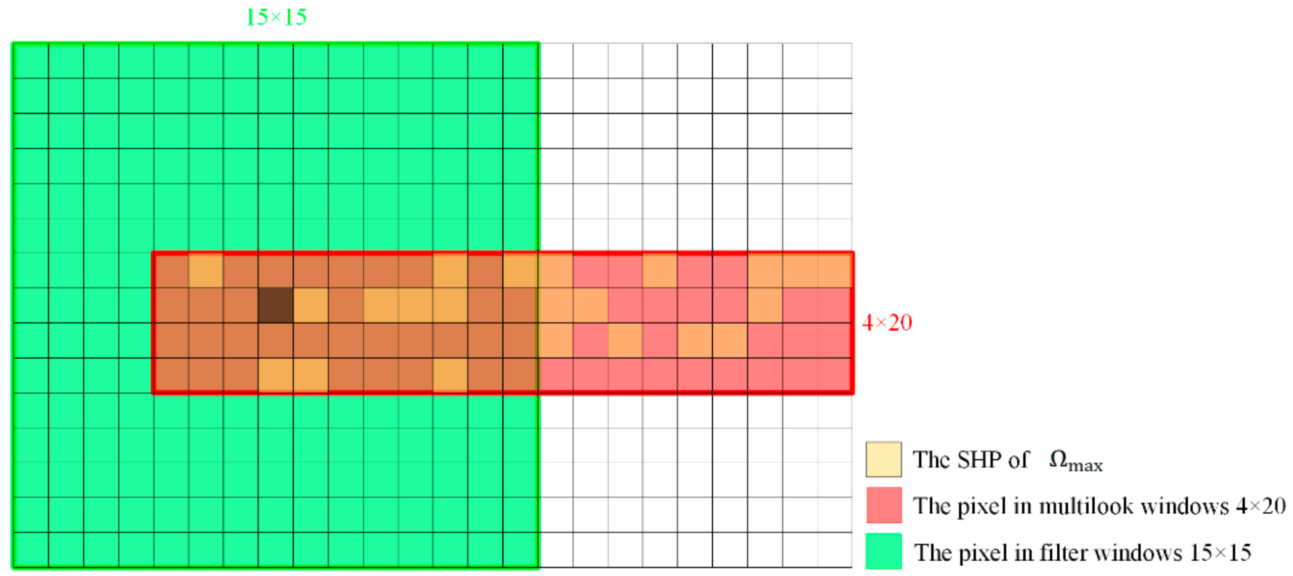
2.2. SHPCs Detection for DSP

Since the mathematical expectation of radar signals is not attainable in practice, under the assumption of distributed targets, coherence is usually estimated by spatially averaging radar echoes in a moving window [45]:

$$\hat{\gamma }=\frac{{\displaystyle \sum _{i=1}^L{s}_{1i}\stackrel{*}{s_{2i}}\cdot e^{j\varphi (i)}}}{\sqrt{{\displaystyle \sum _{i=1}^L{\left|s_{1i}\right|}^2}}\sqrt{{\displaystyle \sum _{i=1}^L{\left|s_{2i}\right|}^2}}}$$

(5)

where i denotes the i-th pixel in a coherence-estimate window (CEW), s₁ and s₂ are complex signals from coregistered InSAR images and ∗ is a complex conjugate operator. For each CEW, L pixels are used to obtain a coherence estimate. $\hat{\gamma }$ is the estimated value of window coherence. The averaging in this method does not consider the homogeneity of neighboring pixels.

Backscattering amplitude statistics are a suitable method for adaptively grouping and averaging pixels in order to preserve the phase signatures of natural structures in the observed area [29]. The AD statistic is powerful at detecting changes in the shape parameter and detecting changes within a scale family [32]. In this paper, the AD test method is used to identify homogeneous pixels based on multitemporal amplitude data:

$${\mathrm{A}}_{M,M}^2=\frac{M}{2}{\displaystyle \sum _{X\in \left.\left\{X_P,i,X_q,i\right.\right\}}\frac{{({\widehat{F}}_p(X)-{\widehat{F}}_q(X))}^2}{{\widehat{F}}_{pq}(X)(1-{\widehat{F}}_{pq}(X))}}$$

(6)

where ${\widehat{F}}_{pq}\left(X\right)$ is the empirical cumulative distribution functions of the pooled distribution obtained by combining the two independent datasets, $X_p, i$ and $X_q,i$, $i=1,\dots ,M$, into dataset $X=\left\{X_p,i,X_q,i\right\}$. The AD test method is used to test each pixel within a multilook window in order to obtain the MSHPC within the multilook window, and the schematic diagram of AD test in multilook window is shown in Figure 1. The pixel number of MSHPC is used to determine whether the window is considered as a candidate DSP, and the steps for selecting a candidate DSP are as follows.

(1) In the multilook windows (size is N*M), for image pixel F (pixel x_i, pixel y_j), by applying the two-sample AD test to amplitude data vectors, other pixels within the window that are considered statistically homogeneous with pixel F are selected given a certain level of significance.

(2) The image pixels in a multilook window that, although selected by the AD test, are not connected to P directly or through other SHPs are discarded.

(3) Repeat steps (1) and (2) for the pixels within the ${\mathrm{window}}_{\mathrm{M}}$ (${\mathrm{window}}_{\mathrm{M}}$ is a multilook window), respectively, where i = 1, 2, 3 … N and j = 1, 2, 3 … M until all pixels in all windows are detected, and the homogeneous cluster$\mathsf{\Omega }=\left[{\mathsf{\Omega }}_1,{\mathsf{\Omega }}_2,{\mathsf{\Omega }}_3....{\mathsf{\Omega }}_{\mathrm{N}\times \mathrm{M}}\right]$ of each individual pixel is obtained.

(4) Judging the pixel number of MSHPC in each cluster, the window for which its pixel number of MSHPC is greater than a certain threshold is the candidate DSP (and the MSHPC are ${\mathsf{\Omega }}_{\max }$).

The above is the method of the candidate DSPs selection. We consider the pixel as a candidate DSP when the pixel number of MSHPC in the multilook window is greater than the threshold. As shown in Figure 2, the yellow pixels in the red box region are the SHPs of the MSHPC in the multilook window. It is worth mentioning that not only the AD test method could be used in testing but also various methods for testing homogeneous pixels can be used for testing. The phase quality of candidate DSP is poor compared to the high coherence region. In order to improve the phase quality of DSP, spatial filtering is performed based on homogeneous pixels after determining DSP with reference to the spatial filtering technique of SqueenSAR. The steps of homogeneous pixel identification for ${\mathrm{SHP}}_{{\mathsf{\Omega }}_{\max }}$ are as follows.

(1) The second homogeneous pixel test was performed for each SHP in ${\mathsf{\Omega }}_{\max }$, and the window size was winA×winR. By using pixel P_max (P_max$\in {\mathsf{\Omega }}_{\max }$) as the central pixel, the intensity vectors of pixel P_max and other pixels q (q$\in {\mathrm{window}}_{\mathrm{F}},{ \mathrm{window}}_{\mathrm{F}}$ as the filter window) in the filter window are tested by using the AD test method to identify SHPs with P_max.

(2) The image pixels in the filter window that, though selected by the AD test, are not connected to P_max directly nor through other SHPs are discarded.

The ${\mathrm{SHP}}_{{\mathsf{\Omega }}_{\max }}$ of DSP and ${\mathrm{SHP}}_{\mathrm{filter}}$ of each${\mathrm{SHP}}_{{\mathsf{\Omega }}_{\max }}$ are selected to prepare coherent estimations for improving the target phase’s quality. Once the proper estimation window has been defined for each image pixel, by carefully selecting SHP families, amplitude data can be despeckled, interferometric phase values can be filtered and coherence values can be estimated properly.

2.3. The Phase Optimization of DSPs

It should be noted that the same ${\mathrm{SHP}}_{\mathrm{filter}}$ will exist in different ${\mathrm{SHP}}_{{\mathsf{\Omega }}_{\max }}$. In the phase estimation, in order to avoid the duplication of the same pixel, the ${\mathrm{SHP}}_{\mathrm{filter}}$ of different ${\mathrm{SHP}}_{{\mathsf{\Omega }}_{\max }}$ should be integrated, and the duplicate ${\mathrm{SHP}}_{\mathrm{coherence}}$ should be removed to obtain the final ${\mathrm{SHP}}_{\mathrm{coherence}}$ for coherent estimation. After identification of the ${\mathrm{SHP}}_{\mathrm{coherence}}$, it is possible to estimate the sample covariance matrix given by the following:

$$C(W)=E\left[d(W)d{(W)}^H\right]\approx \frac{1}{\left|{\mathsf{\Omega }}_{\mathrm{C}}\right|}{\displaystyle \sum _{P\in {\mathsf{\Omega }}_{\mathrm{C}}}d(P)d{(P)}^H}=\widehat{C}$$

(7)

where H indicates Hermitian conjugation, and ${\mathsf{\Omega }}_{\mathrm{C}}$ is the set of ${\mathrm{SHP}}_{\mathrm{coherence}}$ used in the sample estimate of the covariance matrix. $d\left(P\right)={\left[{\mathrm{d}}_1\left(P\right),{\mathrm{d}}_2\left(P\right),\dots {\mathrm{d}}_{\mathrm{N}}\left(P\right)\right]}^H$ is the complex data vector of generic image pixel, and ${\mathrm{d}}_{\mathrm{i}}\left(P\right)$ is the complex reflectivity value of the i-th image of the data-stack corresponding to pixel P. $d\left(W\right)=\left[d{\left(P\right)}_1,d{\left(P\right)}_2,\dots d{\left(P\right)}_{\mathrm{NC}}\right]$ is the complex data vector of the ${\mathrm{SHP}}_{\mathrm{coherence}}$ used to estimate coherence, and NC is the pixel number of ${\mathrm{SHP}}_{\mathrm{coherence}}$. The covariance matrix $\widehat{C}$ is an N × N Hermitian positive semidefinite matrix, with N being the number of SAR images. For phase optimization, suppose that the coherence matrix of multilook windows can be expressed as follows [29].

$$\mathsf{\Gamma }\left(W\right)={\mathsf{\Theta }\mathsf{{\rm Y}}\mathsf{\Theta }}^{\mathrm{H}}$$

(8)

$\mathsf{{\rm Y}}$ is an N × N symmetric real-value matrix for which its elements correspond to the coherence values of all the interferograms. $\mathsf{\Theta }$ is an N × N diagonal matrix containing the values of the “true” phase values of multilook-windows W, related to the optical path of the radar beam in each acquisition. The probability distribution function of the SHP can be expressed as follows [46]:

$$W({\mathrm{d}}_{\mathsf{\Omega }}|\mathbf{\theta })\propto {\displaystyle \prod }_{\mathrm{p}\in \mathsf{\Omega }}\exp \left(-{\mathrm{d}}_{\mathrm{P}}^{\mathrm{H}}{\mathsf{\Theta }\mathsf{{\rm Y}}}^{-1}{\mathsf{\Theta }}^{\mathrm{H}}{\mathrm{d}}_{\mathrm{p}}\right)=\left[-\mathrm{trace}\left({\mathsf{\Theta }\mathsf{{\rm Y}}}^{-1}{\mathsf{\Theta }}^{\mathrm{H}}\widehat{\mathsf{\Gamma }}\right)\right]$$

(9)

where $\mathbf{\theta }={\left[{\theta }_1,{\theta }_2,\dots ,{\theta }_N\right]}^{\mathrm{T}}$ is simply the vector of the phase values of N available images in correspondence to the multilook windows. The estimated result $\theta$ of maximum likelihood (ML) is obtained by maximizing this probability distribution function or minimizing the absolute value of its logarithm [47,48]. The optimal estimate of the N phase values is then given by the following.

$$\begin{array}{cc}\widehat{\theta }& =\underset{\theta }{\arg \max }\left\{\exp [-\mathrm{trace}(\Phi {{\displaystyle \gamma }}^{-1}{\Phi }^H\widehat{\mathsf{\Gamma }}(W))]\right\}\\ & =\underset{\theta }{\arg \max }\left\{\exp [-{\Lambda }^H({{\displaystyle \gamma }}^{-1}\circ \widehat{\mathsf{\Gamma }}(W))\Lambda ]\right\}\\ & =\underset{\theta }{\arg \max }\left\{{\Lambda }^H({{\displaystyle \gamma }}^{-1}\circ \widehat{\mathsf{\Gamma }}(W))\Lambda \right\}\end{array}$$

(10)

$\mathsf{\Phi }$is an N × N diagonal matrix, $\mathsf{\Phi }=\mathrm{diag}\left\{\exp \left(\mathrm{i}\theta \right)\right\}$; Λ is an N-dimensional vector, $\mathsf{\Phi }=\exp \left(\mathrm{i}\theta \right)$ and ° represents the Hadamard product. Therefore, it is necessary to use an iterative method to find the parameters corresponding to the minimization of Equation (9) in order to obtain the optimal phase sequence. However, iterative computation using the BFGS method is extremely time consuming [46]. If an initial value close to the optimal solution is provided, it will greatly increase the speed of iteration.

The EMI method differs from the PTA method by introducing additional degrees of freedom for the estimation in maximizing the Wishart likelihood distribution [49], turning the problem into a biobjective optimization problem. In order to improve computational efficiency, the EMI method reduces the optimization problem to a maximum eigenvector problem by solving the following equation.

$$\left(\hat{\mathsf{\Gamma }}{\left(W\right)}^{-1}\circ C\right){\widehat{\theta }}_{initial}=\lambda {\widehat{\theta }}_{initial}$$

(11)

This is the formulation of eigen decomposition of the Hadamard product ${\widehat{\mathsf{\Gamma }}}^{-1}\circ C$, with λ as the minimum eigenvalue and ${\widehat{\theta }}_{initial}$as its corresponding eigenvector. We use the phase sequence ${\widehat{\theta }}_{initial}$ solved by the EMI method as the initial value for the solution of Equation (9) in order to speed up phase optimization and to enhance the speed of the solution while ensuring the accuracy of the solution. We refer to this method as PTA-EMI. After the optimal phase has been estimated, the phase estimation results need to be evaluated. We evaluate the results by using the temporal coherence estimation method used in the PTA algorithm [29,50].

$$\gamma =\frac{2}{N^2-N}Re{\displaystyle \sum }_{n=1}^N{\displaystyle \sum }_{k=n+1}^N{e}^{i{\varphi }_{nk}}{e}^{-i\left({\vartheta }_n-{\vartheta }_k\right)}$$

(12)

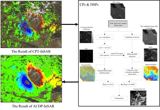
2.4. The Process of ACDP-InSAR

We have described the processing chain of the CPT algorithm, the SHP used to identify the DSP coherence estimate based on the AD algorithm and the optimization of the DSP phase by using the PTA-EMI algorithm. After the coregistration image is processed by the above method, the standard CPT-InSAR processing chain can be used to reproduce the parameters of CPs and DSPs. The flow chart of ACDP-InSAR is shown in Figure 3 and can be described as follows.

(1) The time baseline and the space baseline are used to select the appropriate combination of the interference. The average coherence of the interferometric combination is calculated with an N×M window, and the CPs are selected by setting the coherence threshold.

(2) The operations of preprocessing the magnitude images of N images and then finding the non-CP region and sparse-CP region SHPs based on the method outlined in Section 2.2 are conducted to determine the DSP target and to record the SHP used to estimate the DSP’s coherence matrix.

(3) The estimation of the coherence matrix of the DSP target using SHP and of the optimal phase sequence based on the PTA-EMI is performed as described in Section 2.3.

(4) Based on the phase triangularity and the optimized phase, the phase dataset of DSP under the above interference combination is calculated.

(5) The phase information of CP and DSP are jointly processed according to the CPT processing work chain in order to invert the physical parameters of the measuring point.

Figure 3. Algorithm flow chart of ACDP-InSAR.

Figure 3. Algorithm flow chart of ACDP-InSAR.

The N phase sequences estimated using the PTA-EMI method have the following phase triangularity:

$${\varphi }_{ij}={\theta }_j-{\theta }_i$$

(13)

where ${\varphi }_{ij}$ represents the phase difference between time points i and j; ${\theta }_j$ and${\theta }_i$ represent the phase values between time points i and j. In coherence estimation, complex data are used, and topographic phases should be removed [51]. Compared with the traditional CPT method, the ACDP-InSAR method does not develop a hybrid processing chain but retrieves homogeneous pixels in the low coherence region based on the AD test method in order to obtain the coherence matrix and uses the PTA-EMI method to obtain the optimal phase value for jointly processing CPs and DSPs.

3. Experiment

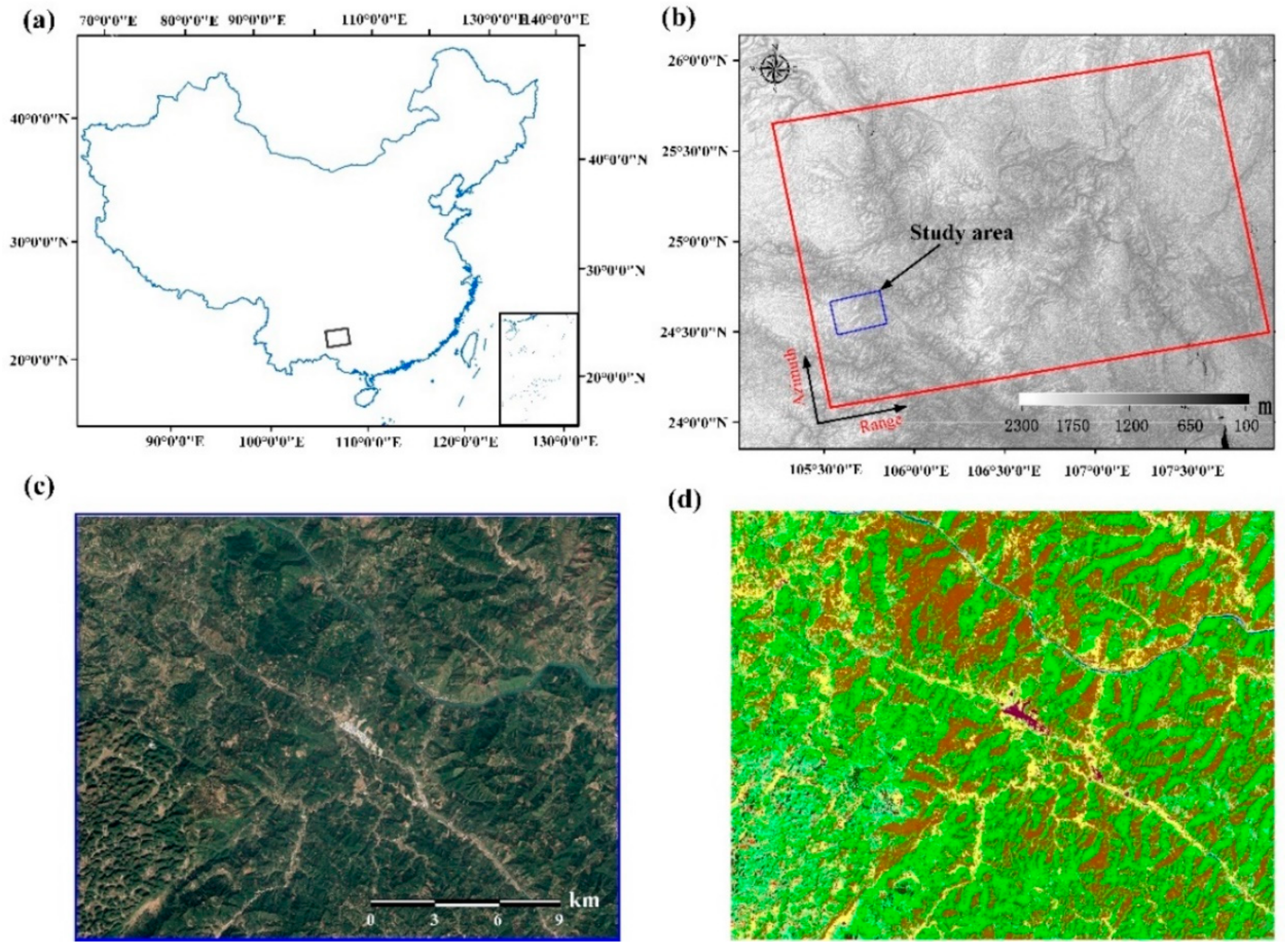
3.1. Case 1: Mountainous Areas in Southwestern China

3.1.1. Study Area and Dataset

The proposed method is validated by 31 descending Sentinel-1 SAR images acquired from 12 October 2018 to 19 October 2019 over mountainous areas in the southern region of Bijie city, Guizhou Province, China (see Figure 4a). Due to rough terrain and vegetation in the area, it is difficult for the conventional CTP-InSAR algorithm. Sentinel-1 SAR is C-band, with its wavelength of 5.6 cm. The nominal resolutions in azimuth and slant-range directions are 5 and 20 m, respectively, corresponding to pixel dimensions of 2.3 and 13.9 m. The SAR image of the study area contains 1600 × 8000 pixels, covering approximately 21 km × 21 km in the azimuth and range directions. Figure 4b shows the TanDEM-X 90 m Digital Elevation Model (DEM) downloaded from the German Aerospace Center (DLR) EOC GEOSERVICE data portal. As observed from Figure 4d, the study area mainly includes impervious, evergreen broadleaved forest, shrubland, evergreen shrubland, rainfed cropland, water bodies and buildings. The results of land use classification are obtained from the Data Sharing and Service Portal supported by the Big Earth Data Science Engineering Program (http://data.casearth.cn/sdo/detail/5d904b7a0887164a5c7fbfa0, accessed on 9 October 2021) [52], and the classification information is shown in

Table 1. Classification Information of Figure 4d.

Number	Classification System	Color
1	Impervious	(195,20,0)
2	Evergreen broadleaved forest	(0,100,0)
3	Shrubland	(150,100,0)
4	Evergreen shrubland	(150,75,0)
5	Rainfed cropland	(255,255,100)
6	Closed deciduous broadleaved forest	(170,200,0)
7	Irrigated cropland	(170,240,240)
8	Water body	(0,70,200)

.

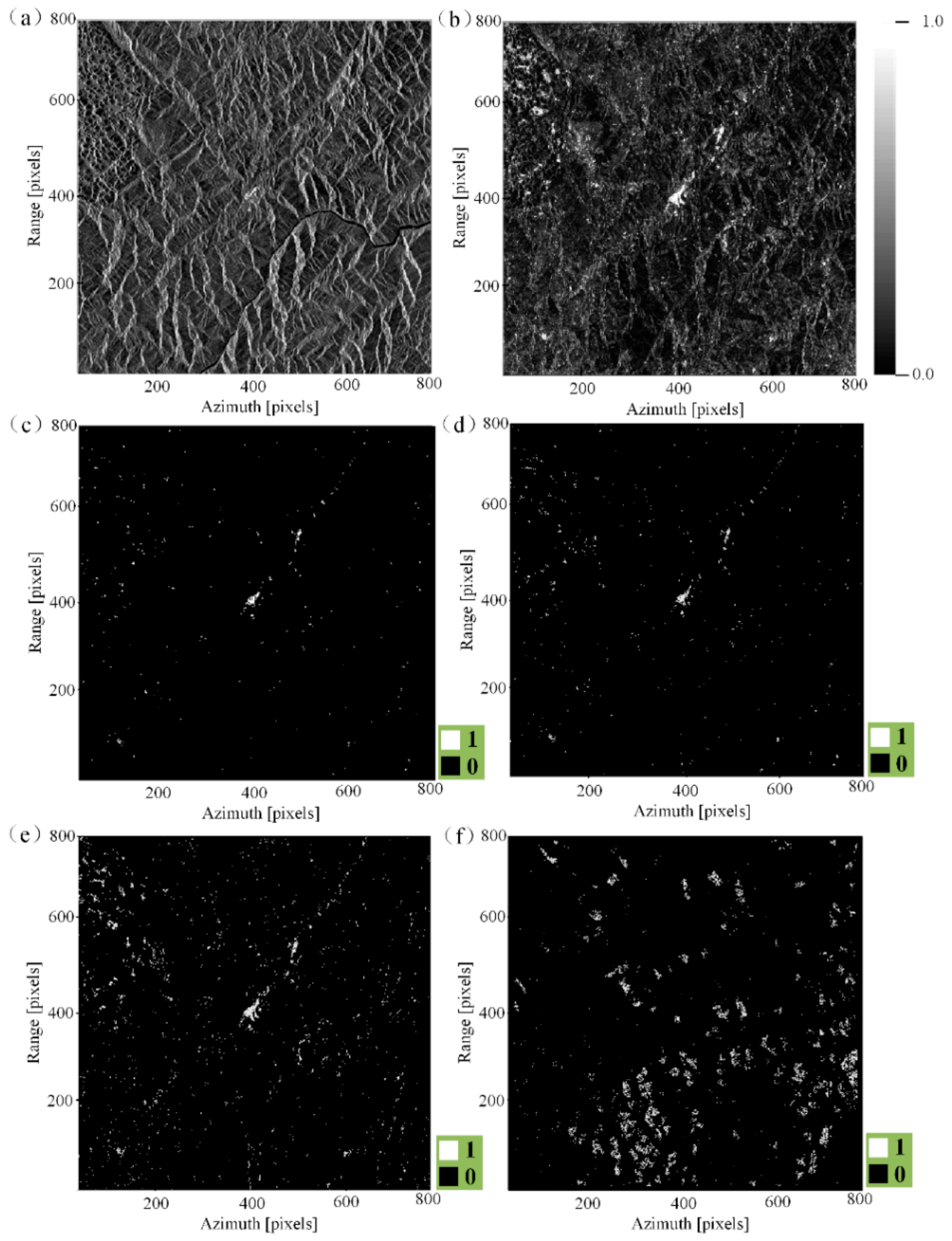
3.1.2. Data Processing and Result

We use TanDEM and precise orbit data to preprocess Sentinel-1 data and then generated the single look complex (SLC) data after coregistration. The date of the main image used in the registration is 12 October 2018, and the amplitude image of the main image is shown in Figure 5a. We follow the steps in Section 2.4 in order to process SLC data. When calculating the average coherence coefficient, the coherence of the interference pairs within a certain baseline threshold and spatial threshold is averaged. The multilook ratio between the azimuth and range is 4:20. The average coherence coefficient of the study area is shown in Figure 5b. According to statistics, the average coherence coefficient of the entire study area is 0.165. When selecting CPs, the coherence threshold is 0.5; that is, the pixels with the average coherence coefficient greater than 0.5 are selected as CPs. The results of the traditional CPs selection method with a coherent threshold at 0.5, 0.375 and 0.25 are shown in Figure 5c,d,e, respectively. In Figure 5c,d and Figure 5e, there are 329, 808 and 1872 coherent pixels, respectively. Although the number of CPs with low threshold is obviously more than the number of CPs with high threshold, the poor phase quality of CPs with low coherence threshold will affect the accuracy of deformation results. Therefore, the coherence threshold of CPs used in this experimental area is 0.5 for deformation inversion. By comparing the spatial relationship between the magnitude map, optical image, land used data and CP, it was observed that CPs are mainly distributed in the built-up areas of the township and on bare rock. It should be noted that the coordinate system in Figure 5 is the SAR coordinate system, while the optical image coordinate system in Figure 4 is the WGS-84 coordinate system.

DSP is extracted by using the method outlined in Section 2.2. First, the amplitude dataset is corrected, and the amplitude value is normalized. The multilook window in the DSP selection is 4:20, and the threshold value of the maximum pixel number of clusters is selected as 48; that is, the window with the maximum pixel number of MSHPC greater than 48 is selected as the candidate DSP. The dimensions of the window used to identify ${\mathrm{SHP}}_{{\mathsf{\Omega }}_{\max }}$ is about four hectares, which corresponds in pixels to a window of 21 × 21. By considering the testing time and the distribution of homogeneous statistical areas, this detection range is reasonable in non-urban areas. The threshold of SHP rejection is 20 in filter window. By fixing 20 as the minimum number of SHP on which spatial filtering can be carried out, it is possible to preserve information of highly coherent targets [29]. Finally, the candidate DSPs were judged based on the pixel number of SHPs: The candidate DSPs below 48 were rejected, and the remaining candidate DSPs are the final DSPs. The results of DSP pixel selection are shown in Figure 5f, with 4499 measuring points. By comparing the spatial relationships of the magnitude map, optical images and DSP, it was found that DSP points were mainly distributed in agricultural fields and submerged vegetation areas. In the experimental area, the number of DSPs was approximately 10 times of the number of CPs with the coherent threshold as 0.5. It should be noted that the effect of monitoring point density enhancement is more related to both topography and geomorphology, and the effect has a better performance in non-urban areas.

In order to show the validity of the PTA-EMI method, we processed data not only possessing DSP but also all pixels. After using PTA-EMI, we acquired N filtered differential interferograms. These N differential interferograms are the optimized phase after spatial filtering and temporal filtering. We selected three interference phases before and after filtering for comparison, as shown in Figure 6. It can be observed that the quality of the interference phase obtained by the proposed method has been greatly improved, which proves the effectiveness of the algorithm. Figure 7 shows the results of temporal coherence calculated according to Equation (11), which takes values in the range of 0–1, with larger values representing better temporal coherence and better temporal phase estimation results. It can be observed from the Figure 7 that the temporal coherence of the county and low vegetation is better, while the temporal coherence of the broadleaf forest is worse.

After optimizing the phase of the DSP pixels, we fuse the CPs and their phase with the DSP pixels and its phase, and the merged pixels are named mixed coherent pixels (MCPs). The phase of the CPs is the original phase and has not been processed by phase optimization. According to the CPT method, the Delauney triangulation [53] of MCPs is constructed and enters the phase, slope distance, incident angle and baseline parameters into the triangulation. Finally, the deformation rate of the MCPs is obtained through integration. The results of the deformation rate based on the CPT method and the deformation rate based on the ACDP-InSAR method in the study area of case 1 are shown in Figure 8. By comparing the two results, it can be observed that the number of measuring points has increased significantly, and the results of the deformation rate are more consistent, which proves the effectiveness and reliability of the algorithm proposed in this paper.

3.2. Case 2: Shigatse M5.9 earthquake in Tibet, China

3.2.1. Study Area and Dataset

The proposed method is validated by 29 descending Sentinel-1 SAR images acquired from 10 January 2020 to 21 December 2020 over the middle Himalayan Mountains (see Figure 9c). The SAR image of the study area contains 2000 × 14000 pixels, covering approximately 31 km × 27 km in the azimuth and range directions. Figure 9a shows the TanDEM-X 90m DEM of the study area, and Figure 9b shows the Sentinel-2 optical images of the study area. The study area is located at the junction of the Indian plate and the Eurasian plate in the Himalayan seismic zone. According to the website of the China Earthquake Networks Center, an earthquake of magnitude 5.9 occurred in Tingri County, Shigatse City, Tibet, on 20 March 2020, and the focal depth was 10.0 km. There have been 134 earthquakes of magnitude three and above within 200 kilometers of the epicenter in the past 9 years. The largest earthquake was a magnitude 7.5 earthquake that occurred in Nepal on 12 May 2015.

3.2.2. Data Processing and Result

The date of the main image used in the coregistration is 8 January 2020, and the amplitude image of the main image is shown in Figure 10a. We follow the steps in Section 2.4 to process the SLC data of the study area in case 2. The multilook ratio between azimuth and range is 4:20. The ground features in this area are mainly grassland and bare rock, with high coherence. Therefore, in order to monitor points with exceptional quality, the coherence threshold is set to 0.6.

DSP is extracted by the method outlined in Section 2.2. The amplitude dataset is corrected after coregistration, and the amplitude value is normalized. Then, the multilook window in the DSP selection is 4:20, and the threshold value of the maximum pixel number of cluster is 48. Then, the homogeneous pixels of the ${\mathrm{SHP}}_{{\mathsf{\Omega }}_{\max }}$ were tested, and the other parameters were the same as those in case 1. The coherence matrix is estimated by SHP, and the phase of DSPs is optimized by the PTA-EMI method. Case 1 has proven that the effect of phase optimization is obvious, and it is no longer verified in this experiment.

The results of the deformation rate based on the CPT method and the deformation rate based on the ACDP-InSAR method in the Shigatse M5.9 earthquake are shown in Figure 11. By comparing both results, it can be observed that the number of measuring point has increased significantly, and the results of the deformation rate are more consistent. The measuring point number of CPs is 14516 and the measuring point number of CPs and DSPs is 95462. The increase in the density of monitoring points allows detecting surface deformations more clearly. It can be observed from Figure 11 that the fault zone of the earthquake is very obvious, and the range and absolute value of surface subsidence on the east side are larger than the range and absolute value of surface uplift on the west side. There is no monitoring point in the center of the deformation field because the deformation gradient is too large, which results in decoherence. From the phase of the interference pair 20200320–20200427, the maximum deformation can be roughly calculated to reach 300 mm. The study area is a medium-high coherence area, but the conventional CPT-InSAR cannot meet the demand for measuring point density for seismic deformation inversion.

4. Discussion

It can be observed from the experimental results that the method proposed in this paper will increase the density of monitoring points and improve phase quality. When detecting SHPs in a double-layer window, the size of the window can be dynamically adjusted. The size of the multilook window depends on the multilook number of the average coherence coefficient, which should be unified; otherwise, CP and DSP cannot be combined. The size of the filtering window will affect the filter’s result. A small window will render the filter unapparent, but a window that is too large induce computational burden and may lose details. In some scenes, the filter window is too large to retrieve more SHPs, which is an invalid operation. Therefore, the corresponding window size should be set according to different application scenarios. In order ensure the homogeneity of multilook windows, a large threshold should be used.

In the era of SAR Big Data, the processing efficiency of algorithms is the basis of big data processing. The PTA-EML method used in this paper has improved efficiency over PTA phase optimization. It should be noted that the algorithm for identifying MSHPC is too redundant when extracting DSPs. The mutuality of hypothesis testing can be used to enhance the speed of the MSHPC test. Mutuality of AD test means that the test result between data group B and data group A when A as main body is the same as the test result when B as the main body. It is not necessary to examine each pixel when retrieving MSHPC in multilook windows, because the SHPCs of pixel A and the SHPC of A’s SHP are practically the same. Therefore, it is only necessary to classify the pixels in the window by their statistical characteristics, and the cluster with the largest pixel number is the MSHPC of this window.

Phase optimization is a more time-consuming step [37], and the pixel number of DSPs selected by ACDP-InSAR in mulitilook scenes is much smaller than the pixel number of DS points selected by SqueenSAR in the single-look scenes. Therefore, the processing speed of the proposed method is faster than that of the conventional SqueenSAR algorithm. Taking case 1 as an example, we counted the time consumed by ACDP-InSAR and SqueenSAR in SHP selection and phase-link steps. The statistical diagram of algorithm running time is shown in Figure 12. The diagram shows, in Figure 12, that the processing speed of ACDP-InSAR in SHP selection is lower than that of SqueenSAR, and the processing speed of the phase link is higher than that of SqueenSAR. The overall processing speed of the method proposed in this paper significantly improved. On the other hand, the proposed method has a cost of resolution reduction. The ACDP-InSAR method is more suitable for high precision surface deformation monitoring in large spatial scales.

In Section 3, we used two experiments to prove effectiveness in non-urban areas, which has a good effect of increasing the number of points. Unfortunately, no in situ measurement data could be applied to quantitatively verify the accuracy of the algorithm in t experiment areas. In order to quantitatively evaluate the algorithm accuracy proposed in this paper, the measurement data for Beijing, China, was used. The field observation points covering 40 different regions in Beijing, China, from 2017 to 2018 were collected. However, the measurement period of the measured leveling data is one year, which cannot be compared with the InSAR results in a long time series. We changed the leveling data into annual average settlement and compared it with the annual average deformation rate of ACDP-InSAR. Before comparison, the vertical deformation of leveling data was changed into the deformation along the LOS direction according to satellite parameters. The area of accuracy verification and data comparison between leveling data and ACDP-InSAR result are shown in Figure 13 and Figure 14, respectively.

As observed from Figure 13c, the leveling results are practically consistent with the results of ACDP-InSAR, and individual field observation points are different. The specific data values are compared, as shown in Figure 14. According to statistics, the root mean square error (RMSE) between ACDP-InSAR results and leveling data is 5.45 mm/year, which proves that ACDP-InSAR results are reliable.

The ACDP-InSAR method not only has the advantages of the CPT-InSAR method but also has better density with respect to measuring points and detectability than those of the latter method. Of course, the ACDP-InSAR method also has some limitations. Firstly, ACDP-InSAR is an improvement of the CPT-InSAR method, which estimates coherent values by multilook processing; thus, it will degrade resolution. Low resolution is not suitable for fine deformation measurement, such as deformation monitoring of dams, bridges and regional buildings. Secondly, both the ACDP-InSAR method and the CPT-InSAR method solve the results by constructing a network. In large spatial scale deformation monitoring, the process of removing edges with low coherence and causing a set of CPs to be divided into several clusters is easy. Future investigations should establish a multi-layer network to connect multiple clusters during large spatial scale data processing in order to ensure the consistency of regional deformation monitoring.

5. Conclusions

In this paper, we proposed method ACDP-InSAR method in order to improve measuring point density based on distributed scattering targets for solving the problem of sparse measurement points in non-urban areas caused by CPT-InSAR. ACDP-InSAR identifies SHPs with two-layer windows based on the AD test. The first multilook window selects the DSP, and the second filter window determines the SHPCs of the DSP. The CP target is selected on the coherence coefficient map after multilooking, while the DSP needs to be selected under the single-look scene. Therefore, the resolution of DSP should be consistent with that of CP. The SHP of DSP is used to estimate the coherence matrix of DSP, the PTA-EMI method is then used to optimize phase sequences, and a set of optimal phase sequence with phase triangularity is obtained. We selected two regions as experimental areas located in the mountainous region of Southwest China and around Shigatse on the Tibet Plateau. The experimental results show that the density of monitoring points increases approximately 5–10 times, and the phase quality is improved, verifying the effectiveness and applicability of the algorithm. The ACDP-InSAR method can not only acquire monitoring points in a low-coherence region but also increase the density of monitoring points in a medium-coherence region. The root mean square error (RMSE) between ACDP-InSAR results and leveling data is 5.45 mm/y, which proves that ACDP-InSAR results are reliable. Compared with the conventional DS-InSAR technology, this method improves processing speed at the cost of resolution loss and is suitable for Earth surface movement monitoring in large spatial scales.

References

1. Samsonov, S.; d’Oreye, N.; Smets, B. Ground deformation associated with post-mining activity at the French-German border revealed by novel InSAR time series method. Int. J. Appl. Earth Obs. 2013, 23, 142–154. [Google Scholar] [CrossRef]
2. Lu, Z.; Dzurisin, D. InSAR Imaging of Aleutian Volcanoes[M]//InSAR Imaging of Aleutian Volcanoes; Springer: Berlin/Heidelberg, Germany, 2014; pp. 87–345. [Google Scholar]
3. Wang, C.; Zhang, Z.; Zhang, H.; Wu, Q.; Zhang, B.; Tang, Y. Seasonal deformation features on Qinghai–Tibet railway observed using time-series InSAR technique with high-resolution TerraSAR-X images. Remote Sens. Lett. 2017, 8, 1–10. [Google Scholar] [CrossRef]
4. Wang, C.; Zhang, Z.; Zhang, H.; Zhang, B.; Tang, Y.; Wu, Q. Active Layer Thickness Retrieval of Qinghai–Tibet Permafrost Using the TerraSAR-X InSAR Technique. IEEE J. Sel. Top. Appl. Earth Obs. Remote Sens. 2018, 11, 4403–4413. [Google Scholar] [CrossRef]
5. Wang, J.; Wang, C.; Zhang, H.; Tang, Y.; Zhang, X.; Zhang, Z. Small-Baseline Approach for Monitoring the Freezing and Thawing Deformation of Permafrost on the Beiluhe Basin, Tibetan Plateau Using TerraSAR-X and Sentinel-1 Data. Sensors 2020, 20, 4464. [Google Scholar] [CrossRef]
6. Hartwig, M.E.; Paradella, W.R.; Mura, J.C. Detection and monitoring of surface motions in active open pit iron mine in the Amazon Region, using persistent scatterer interferometry with terrasar-x satellite data. Remote Sens. 2013, 5, 4719–4734. [Google Scholar] [CrossRef] [Green Version]
7. Zhao, C.; Lu, Z.; Zhang, Q. Time-series deformation monitoring over mining regions with SAR intensity -based offset measurements. Remote Sens. Lett. 2013, 4, 436–445. [Google Scholar] [CrossRef]
8. Lu, Z.; Dzurisin, D.; Biggs, J.; Wicks, C., Jr.; McNutt, S. Ground surface deformation patterns, magma supply, and magma storage at Okmok volcano, Alaska, from InSAR analysis: 1. Intereruption deformation, 1997–2008. J. Geophys. Res. Solid Earth 2010, 115. [Google Scholar] [CrossRef] [Green Version]
9. Dong, L.; Wang, C.; Tang, Y.; Tang, F.; Zhang, H.; Wang, J.; Duan, W. Time Series InSAR Three-Dimensional Displacement Inversion Model of Coal Mining Areas Based on Symmetrical Features of Mining Subsidence. Remote Sens. 2021, 13, 2143. [Google Scholar] [CrossRef]
10. Zebker, H.A.; Villasenor, J. Decorrelation in interferometric radar echoes. IEEE Trans. Geosci. Remote Sens. 1992, 30, 959. [Google Scholar] [CrossRef] [Green Version]
11. Massonnet, D.; Feigl, K.L. Radar interferometry and its application to changes in the Earth's surface. Rev. Geophys. 1998, 36, 441–500. [Google Scholar] [CrossRef] [Green Version]
12. Ferretti, A.; Prati, C.; Rocca, F. Permanent scatterers in SAR interferometry. IEEE Trans. Geosci. Remote Sens. 2001, 39, 8–20. [Google Scholar] [CrossRef]
13. Ferretti, A.; Prati, C.; Rocca, F. Nonlinear subsidence rate estimation using permanent scatterers in differential SAR interferometry. IEEE Trans. Geosci. Remote Sens. 2000, 38, 2202–2212. [Google Scholar] [CrossRef] [Green Version]
14. Ferretti, A.; Prati, C.; Rocca, F. Process for Radar Measurements of the Movement of City Areas and Landsliding Zones; International Application Published Under the Patent Cooperation Treaty (PCT): Washington, DC, USA, 2000.
15. Berardino, P.; Fornaro, G.; Lanari, R.; Sansosti, E. A new algorithm for surface deformation monitoring based on small baseline differential SAR interferograms. IEEE Trans. Geosci. Remote Sens. 2002, 40, 2375–2383. [Google Scholar] [CrossRef] [Green Version]
16. Mora, O.; Mallorqui, J.J.; Broquetas, A. Linear and nonlinear terrain deformation maps from a reduced set of interferometric SAR images. IEEE Trans. Geosci. Remote Sens. 2003, 41, 2243–2253. [Google Scholar] [CrossRef]
17. Mallorquí, J.J.; Mora, O.; Blanco, P. Linear and non-linear long-term terrain deformation with DInSAR (CPT: Coherent Pixels Technique). In Proceedings of the FRINGE 2003 Workshop ESA, Frascati, Italy, 1–5 December 2003; Volume 36, pp. 1–8. [Google Scholar]
18. Blanco, P.; Mallorqui, J.; Duque, S. Advances on DInSAR with ERS and ENVISAT data using the coherent pixels technique (CPT). In Proceedings of the 2006 IEEE International Symposium on Geoscience and Remote Sensing, Denver, CO, USA, 31 July–4 August 2006; pp. 1898–1901. [Google Scholar]
19. Blanco-Sanchez, P.; Mallorquí, J.J.; Duque, S. The coherent pixels technique (CPT): An advanced DInSAR technique for nonlinear deformation monitoring. In Earth Sciences and Mathematics; Birkhäuser: Basel, Switzerland, 2008; pp. 1167–1193. [Google Scholar]
20. Duque, S.; Mallorqui, J.J.; Blanco, P. Application of the coherent pixels technique (CPT) to urban monitoring. In Proceedings of the 2007 Urban Remote Sensing Joint Event, Paris, France, 11–13 April 2007; pp. 1–7. [Google Scholar]
21. Navarro-Hernánde, M.I.; Tomás, R.; Lopez-Sanchez, J.M. Spatial Analysis of Land Subsidence in the San Luis Potosi Valley Induced by Aquifer Overexploitation Using the Coherent Pixels Technique (CPT) and Sentinel-1 InSAR Observation. Remote Sens. 2020, 12, 3822. [Google Scholar] [CrossRef]
22. Costantini, M.; Ferretti, A.; Minati, F. Analysis of surface deformations over the whole Italian territory by interferometric processing of ERS, Envisat and COSMO-SkyMed radar data. Remote Sens. Environ. 2017, 202, 250–275. [Google Scholar] [CrossRef]
23. Bovenga, F.; Nutricato, R.; Guerriero, A.R.L. SPINUA: A flexible processing chain for ERS/ENVISAT long term interferometry. In Proceedings of the Envisat & ERS Symposium, Salzburg, Austria, 6–10 September 2005; p. 572. [Google Scholar]
24. Costantini, M.; Falco, S.; Malvarosa, F. A new method for identification and analysis of persistent scatterers in series of SAR images. In Proceedings of the IGARSS 2008-2008 IEEE International Geoscience and Remote Sensing Symposium, Boston, MA, USA, 7-11 July 2008; Volume 2, pp. II-449–II-452. [Google Scholar]
25. Devanthéry, N.; Crosetto, M.; Monserrat, O.; Cuevas-González, M.; Crippa, B. An approach to persistent scatterer interferometry. Remote Sens. 2014, 6, 6662–6679. [Google Scholar] [CrossRef] [Green Version]
26. Hooper, A. A multi-temporal InSAR method incorporating both persistent scatterer and small baseline approaches. Geophys. Res. Lett. 2008, 35. [Google Scholar] [CrossRef] [Green Version]
27. Rocca, F. Modeling interferogram stacks. IEEE Trans. Geosci. Remote Sens. 2007, 45, 3289–3299. [Google Scholar] [CrossRef]
28. Zebker, H.A.; Shanker, A.P. Geodetic Imaging with Time Series Persistent Scatterer InSAR; American Geophysical Union: San Francisco, CA, USA, 2008; p. G51C-02. [Google Scholar]
29. Ferretti, A.; Fumagalli, A.; Novali, F.; Prati, C.; Rocca, F.; Rucci, A. A new algorithm for processing interferometric data-stacks: SqueeSAR. IEEE Trans. Geosci. Remote Sens. 2011, 49, 3460–3470. [Google Scholar] [CrossRef]
30. Ansari, H.; De Zan, F.; Bamler, R. Efficient phase estimation for interferogram stacks. IEEE Trans. Geosci. Remote Sens. 2018, 56, 4109–4125. [Google Scholar] [CrossRef]
31. Ansari, H.; De Zan, F.; Bamler, R. Sequential Estimator: Toward Efficient InSAR Time Series Analysis. IEEE Trans. Geosci. Remote Sens. 2017, 55, 5637–5652. [Google Scholar] [CrossRef] [Green Version]
32. Wang, G.; Xu, B.; Li, Z. A phase optimization method for DS-InSAR Based on SKP decomposition from quad-polarized data. IEEE Geosci. Remote Sens. Lett. 2021, 1–5. [Google Scholar] [CrossRef]
33. Lilliefors, H.W. On the kolmogorov-smirnov test for normality with mean and variance unknown. J. Am. Stat. Assoc. 1967, 62, 399–402. [Google Scholar] [CrossRef]
34. Razali, N.M.; Wah, Y.B. Power comparisons of shapiro-wilk, kolmogorov-smirnov, lilliefors and anderson-darling tests. J. Stat. Model. Anal. 2011, 2, 21–33. [Google Scholar]
35. Parizzi, A.; Brcic, R. Adaptive InSAR stack multilooking exploiting amplitude statistics: A comparison between different techniques and practical results. IEEE Geosci. Remote Sens. Lett. 2010, 8, 441–445. [Google Scholar] [CrossRef] [Green Version]
36. Polzehl, J.; Spokoiny, V. Propagation-separation approach for local likelihood estimation. Probab. Theory Relat. Fields 2006, 135, 335–362. [Google Scholar] [CrossRef] [Green Version]
37. Deledalle, C.A.; Denis, L.; Tupin, F. NL-InSAR: Nonlocal interferogram estimation. IEEE Trans. Geosci. Remote Sens. 2010, 49, 1441–1452. [Google Scholar] [CrossRef]
38. Anderson, T.W. On the distribution of the two-sample Cramervon Mises criterion. Ann. Math. Stat. 1962, 33, 1148–1159. [Google Scholar] [CrossRef]
39. Jiang, M.; Ding, X.; Hanssen, R.F.; Malhotra, R.; Chang, L. Fast statistically homogeneous pixel selection for covariance matrix estimation for multitemporal InSAR. IEEE Trans. Geosci. Remote Sens. 2014, 53, 1213–1224. [Google Scholar] [CrossRef]
40. Jiang, M.; Guarnieri, A.M. Distributed scatterer interferometry with the refinement of spatiotemporal coherence. IEEE Trans. Geosci. Remote Sens. 2020, 58, 3977–3983. [Google Scholar] [CrossRef]
41. Cao, N.; Lee, H.; Jung, H.C. A phase-decomposition-based PSInSAR processing method. IEEE Trans. Geosci. Remote Sens. 2015, 54, 1074–1090. [Google Scholar] [CrossRef]
42. Fornaro, G.; Verde, S.; Reale, D.; Pauciullo, A. CAESAR: An approach based on covariance matrix decomposition to improve multibaseline–multitemporal interferometric SAR processing. IEEE Trans. Geosci. Remote Sens. 2014, 53, 2050–2065. [Google Scholar] [CrossRef]
43. Liao, M.; Balz, T.; Rocca, F.; Li, D. Paradigm changes in Surface-Motion estimation from SAR: Lessons from 16 years of Sino-European cooperation in the dragon program. IEEE Geosci. Remote Sens. Mag. 2020, 8, 8–21. [Google Scholar] [CrossRef]
44. Xu, W.; Cumming, I. A region-growing algorithm for InSAR phase unwrapping. IEEE Trans. Geosci. Remote Sens. 1999, 37, 124–134. [Google Scholar] [CrossRef] [Green Version]
45. Touzi, R.; Lopes, A.; Bruniquel, J. Coherence estimation for SAR imagery. IEEE Trans. Geosci. Remote Sens. 1999, 37, 135–149. [Google Scholar] [CrossRef] [Green Version]
46. Guarnieri, A.M.; Tebaldini, S. On the exploitation of target statistics for SAR interferometry applications. IEEE Trans. Geosci. Remote Sens. 2008, 46, 3436–3443. [Google Scholar] [CrossRef]
47. Lv, X.; Yazıcı, B.; Zeghal, M. Joint-scatterer processing for time-series InSAR. IEEE Trans. Geosci. Remote Sens. 2014, 52, 7205–7221. [Google Scholar]
48. Samiei-Esfahany, S.; Martins, J.E.; Van, L.F. Phase estimation for distributed scatterers in InSAR stacks using integer least squares estimation. IEEE Trans. Geosci. Remote Sens. 2016, 54, 5671–5687. [Google Scholar] [CrossRef] [Green Version]
49. Goodman, N.R. Statistical analysis based on a certain multivariate complex Gaussian distribution (an introduction). Ann. Math. Stat. 1963, 34, 152–177. [Google Scholar] [CrossRef]
50. Shanker, P.; Zebker, H. Persistent scatterer selection using maximum likelihood estimation. Geophys. Res. Lett. 2007, 34. [Google Scholar] [CrossRef]
51. Cao, N.; Lee, H.; Jung, H.C. Mathematical framework for phase-triangulation algorithms in distributed-scatterer interferometry. IEEE Geosci. Remote Sens. Lett. 2015, 12, 1838–1842. [Google Scholar]
52. Zhang, X.; Liu, L.; Chen, X.; Xie, S.; Gao, Y. Fine Land-Cover Mapping in China Using Landsat Datacube and an Operational SPECLib-Based Approach. Remote Sens. 2019, 11, 1056. [Google Scholar] [CrossRef] [Green Version]
53. Delaunay, B. Sur la sphere vide. Izv. Akad. Nauk SSSR 1934, 7, 1–2. [Google Scholar]
Figure 1. Process of MSHPC acquisition. After testing all pixels in the window, the SHPCs, which have the maximum pixel number of SHPs, include MSHPC.
Remotesensing 13 04784 g001
Figure 2. Example of the double-layer hypothesis testing window. The red window is the multilook window, the yellow pixels are the SHPs of the multilook window and the green window is the spatial filtering window of a single SHP.
Remotesensing 13 04784 g002
Figure 4. (a) The location of Sentinel-1 data in China, and the black box represents range of Sentinel-1. (b) Geographic location of the coverage of the SAR acquisitions superposed on the TanDEM, and the blue box represents the range of Sentinel-1 data. (c) The optical image of study area, and (d) is the classification result of land used in the study area.
Remotesensing 13 04784 g004
Figure 5. (a) Magnitude image of the master image where the date is 20181012. (b) Average coherence coefficient of an interference pair. (c) CPs’ spatial distribution with a coherent threshold as 0.5. (d) CPs’ spatial distribution with a coherent threshold as 0.375. (e) CPs’ spatial distribution with a coherent threshold as 0.25. (f) DSPs’ spatial distribution. The white pixel (value as 1) represents the measuring point of CPs and DSPs in (cf).
Remotesensing 13 04784 g005
Figure 6. (ac) are the original phases of interference pairs 20191007–20191019, 20190913–20191019 and 20190209–20190317, respectively. (df) Phases 20191007–20191019, 20190913–20191019 and 20190209–20190317 after ACDP-InSAR processing.
Remotesensing 13 04784 g006
Figure 7. Time coherence of the study area in mountainous areas.
Remotesensing 13 04784 g007
Figure 8. (a) The surface deformation rate of the study area obtained by the CPT method. (b) The surface deformation rate of the study area obtained by the method proposed in this paper.
Remotesensing 13 04784 g008
Figure 9. (a) The location of Sentinel-1 data in China, and the black box represents range of Sentinel-1. (b) Geographic location of the coverage of the SAR acquisitions superposed on the TanDEM, and the blue box represents the range of Sentinel-1 data. (c) Optical image of the study area of Shigatse M5.9 earthquake in Tibet, China.
Remotesensing 13 04784 g009
Figure 10. (a) Magnitude image of the master image 20200108. (b) Average coherence coefficient of the interference pair.
Remotesensing 13 04784 g010
Figure 11. (a) The surface deformation rate of the study area in case 2 obtained by the CPT-In- SAR method. (b) The surface deformation rate of the study area in case 2 obtained by the method proposed in this paper.
Remotesensing 13 04784 g011
Figure 12. Cumulative processing time of the ACDP-InSAR and SqueenSAR over case 1 as an assessment of computational efficiency.
Remotesensing 13 04784 g012
Figure 13. The experimental area for ACDP-InSAR accuracy verification. (a) The location of the experimental area, and blue box represents the range of leveling data. (b) Distribution map of field observation points. Each benchmark in the figure has a corresponding label, and the color of each field observation point represents the annual average deformation rate obtain from leveling data. The corresponding color label is same as the color label in (c). The result of overlaying the level data deformation rate above the ACDP-InSAR deformation rate.
Remotesensing 13 04784 g013
Figure 14. Comparison between in situ leveling measurements and InSAR results estimated by the proposed method over the field observation points in Figure 13b.
Remotesensing 13 04784 g014