Significant Wave Height Estimation Using Multi-Satellite Observations from GNSS-R

Abstract

This study proposes a significant wave height (SWH) retrieval method based on multi-satellite observations using Global Navigation Satellite System Reflectometry (GNSS-R). The algorithm obtains the signal-to-noise ratio (SNR) through delay-Doppler maps (DDMs) and introduces an offset correction that combines the differences between the elevation angles of multi-satellites. The correction improves the correlation between SNR and SWH and thus enables the estimation of SWH. The feasibility of the proposed algorithm was verified by experiments and a performance comparison with the traditional estimation method based on SNR. The estimation results of the proposed algorithm, with a mean absolute percentage error of 8.26%, a root mean square error of 0.1671 m, and a maximum error of 0.32 m, better matched the true values than the traditional SNR-based method. The method is intended to improve the retrieval accuracy of SWH based on the GNSS-R technique, and to provide services for sea-state information monitoring and ship navigation.

1. Introduction

The ocean occupies approximately 71% of the earth. Marine navigation, marine disaster warnings, ocean-going and polar navigation all require accurate ocean state information [1]. Therefore, marine environment detection has great application value and strategic significance. Sea surface wind fields, significant wave height (SWH), and sea targets are important physical parameters that reflect the sea-state and navigation environment. Traditionally, maritime information is acquired by marine stations, synthetic aperture radar (SAR), radar altimeters, unmanned aerial vehicles (UAVs)-borne measurements and other active observational approaches [2,3,4,5,6,7,8]. Global Navigation Satellite System Reflectometry (GNSS-R) is a new type of remote sensing technology with all-weather operability, multi-source signals, small weight and volume, low power consumption, and low cost. GNSS-R is a more passive detection technology than traditional radars [9,10,11].

GNSS-R uses the L-band signals of US global positioning system (GPS) [12], the Russian global orbiting navigational satellite system (GLONASS) [13], the Galileo system [14] of the European Space Agency (ESA), and the BeiDou Navigation Satellite System (BDS) of China [15] as the signal source. The features of the ocean surface are inferred from the signal reflection characteristics of the surface. Since the 1990s, GNSS-R technology has gradually developed into a new hotspot in the remote sensing field [16]. Subsequent GNSS-R experiments and related researches have been conducted in countries around the world. For example, the Surrey Satellite Technology Ltd. UK-DMC (the United Kingdom-Disaster Monitoring Constellation) satellite was the first experiment to successfully provide available GNSS-R data [17,18]. Following the UK-DMC, the TechDemoSat-1 (TDS-1), launched in 2014, has acquired a large amount of further GNSS-R data [19]. NASA (National Aeronautics and Space Administration)’s CYGNSS (Cyclone Global Navigation Satellite System) mission has launched eight low-orbit satellites for typhoon observations and disaster-impact reductions in typhoon-stricken areas worldwide [20,21]. At present, the GNSS-R technique has been applied to wind fields, SWH, sea ice, ocean altimetry measurements, soil moisture, and other researches [22,23,24,25,26,27,28].

In ocean remote sensing, accurate sea-state information plays a crucial role in ship scheduling, navigation safety, and information perception. The SWH represents the mean height of the largest third of the wave heights arranged in descending order, which is close to the visual wave height [29]. Furthermore, it is an important indicator of sea conditions. As a key application of the GNSS-R technique, SWH estimation has attracted significant research interest. A typical SWH retrieval method is interferometric complex field (ICF), which has been widely used in GNSS-R ocean remote sensing [30,31,32]. Alberto et al. presented the results of a three-mouth field campaign that retrieved the SWH using the interference pattern technique (IPT) and extracted the mean sea surface level (MSSL) from the observed interference patterns [24]. Referring to the SWH measurement method used by radar, an SWH estimation method based on the signal-to-noise ratio (SNR) can be introduced into GNSS-R. The present work attempts to obtain the SNR applicable to GNSS-R and improve the correlation between SNR and SWH using the delay-Doppler maps (DDMs) derived from two BeiDou satellite observations, thereby realizing an improved SWH retrieval method. This paper is divided into four parts. Section 2 presents the principle of the improved algorithm. Section 3 describes the experiments and discusses the experimental results. Section 4 summarizes the conclusions of this paper.

2. Materials and Methods

2.1. GNSS-R Geometry

As shown in Figure 1, GNSS satellites act as transmitters. Their direct signals are captured by the receiver, and their reflected signals pass through the reflection point and multiple scattering points, forming a bistatic radar mode for transmitting and receiving [11]. In one satellite, the receiver can obtain multiple scattered signals along with the direct signal, and the corresponding scattered power can be presented with different delays and Doppler shifts. This 2D mapping, known as a DDM, is the basis of SWH retrieval.

2.2. Algorithm Principle

In SWH retrieval, the SNR changes of the reflected signal contain the information of different sea-states. Based on the DDMs obtained by GNSS-R observations, we here provide the concepts and calculation methods of SNRs in GNSS-R data. The useful information power is obtained as the sum of relative powers in the peak area of the DDM. The noise floor is defined in [33], and the ratio of the two parameters is called the accumulated DDM-to-noise ratio (ADNR):

$$ADNR=\frac{{\displaystyle \sum _{m=1}^M{\displaystyle \sum _{n=1}^{N}DDM\left(t_m,f_n\right)}}-Noise}{Noise}$$

(1)

where $DDM\left(t_m,f_n\right)$ is the power value at a time delay of $t_m$ and a Doppler frequency of $f_n$. $Noise$ is the average power of noise floor in the corresponding DDM. In this paper, $t_m\in \left[-2.0,2.8\right]$ chips, $f_n\in \left[-500,500\right]$ Hz. $m$ and $n$ are the index of delay and Doppler, respectively, $m\in \left[1,48\right]$, $n\in \left[1,15\right]$.

During the experiments, we found that the ADNR values of the same SWH fluctuated at different satellite elevation angles. This fluctuation characteristic increased the deviation of the SWH estimation. Figure 2 plots the relationship between elevation angle and ADNR for an SWH of 2 m. The ADNR was a decreasing function of elevation angle.

The experimental results were fitted to the following formula:

$$f\left(\theta \right)=6.9542\times {\sin }^2(\theta )-23.7790\times \sin (\theta )+22.1739$$

(2)

To reduce the influence of the fluctuation difference, this study proposed an offset correction to ADNR, given as

$$ADN{R}_{*}=ADNR+{\mathrm{\Delta }}_i$$

(3)

In (3), $i$ is the current satellite; the ${\mathrm{\Delta }}_i$ is determined using a second satellite elevation angle and is defined as

$${\mathrm{\Delta }}_i=\frac{ADN{R}_i-ADN{R}_j}{f\left({\theta }_i\right)-f\left({\theta }_j\right)}\times \left(5.907-f\left({\theta }_i\right)\right)$$

(4)

where $ADN{R}_i$ and $ADN{R}_j$ are the ADNR values of the i-th and j-th satellites, respectively, ${\theta }_i$ and ${\theta }_j$ are their corresponding elevation angles.

For convenience of discussion and presentation, the offset and corrected ADNR (called $ADN{R}_{*}$) is also referred to as $ADNR$ in the remainder of this paper.

Based on the above definition, the SWH retrieval model is given as

$$SWH=\left[abc\right]\left[\begin{array}{l}ADN{R}^2\\ ADNR\\ ones\end{array}\right]$$

(5)

where a, b, and c are undetermined coefficients, and $ones$ is the unit matrix.

Letting $K=\left[abc\right]$ and $X={\left[ADN{R}^{2}ADNRones\right]}^T$, and applying the normal equation, $K$ is given by

$$\begin{array}{cc}& KX=SWH\\ \Rightarrow & KX{X}^T=\left(SWH\right)X^T\\ \Rightarrow & KX{X}^T{\left(X{X}^T\right)}^{-1}=\left(SWH\right)X^T{\left(X{X}^T\right)}^{-1}\\ \Rightarrow & K=\left(SWH\right)X^T{\left(X{X}^T\right)}^{-1}\end{array}$$

(6)

The flow of the entire algorithm is illustrated in Figure 3 below.

3. Results and Discussion

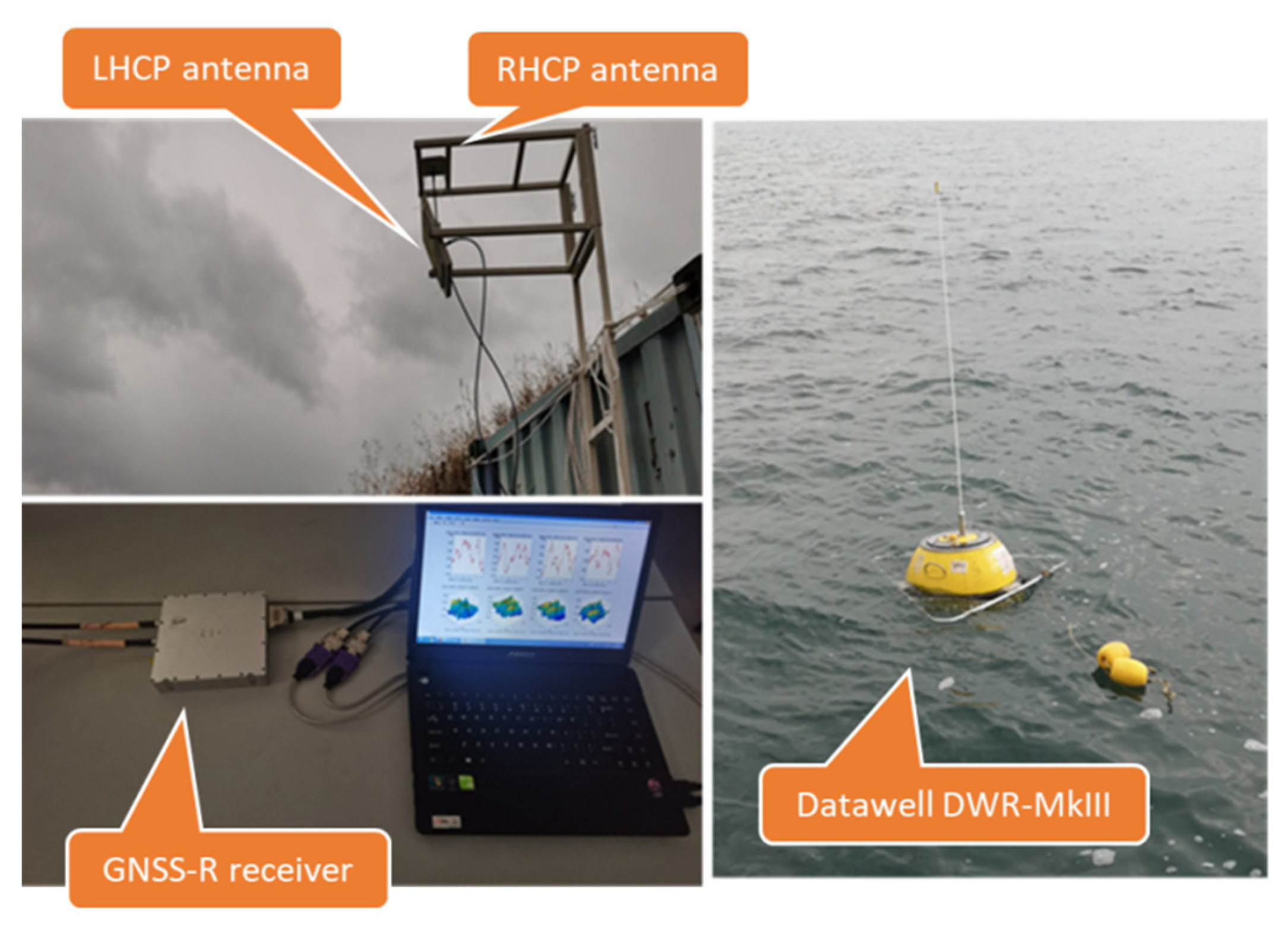
3.1. Experimental Data

To verify the feasibility of the algorithm, GNSS-R experiments were conducted in Lvshun, Dalian (China) in December 2020. As comparison data, we also acquired the instantaneous SWH measurements provided by the Datawell’s Directional Waverider buoy (Datawell DWR-MkIII), as shown in the right of Figure 4. The measurements recorded using the buoy include maximum wave height (Hmax), mean height of the highest 1/10 of the waves (H[1/10]), mean height of the highest third of the waves (H[1/3]), and mean height of all waves (Hav). According to the definition of significant wave height (SWH), this study selected the parameter “H[1/3]” as true value data. The location and antenna installations of the experimental observations are shown in Figure 4 and Figure 5, respectively. The entire observation system includes a right hand circularly polarized (RHCP) zenith antenna with a peak gain of 3 dBi, a left hand circularly polarized (LHCP) downward pointing with a peak gain of 12 dBi, and a GNSS-R receiver. This system can capture the BeiDou satellite signal on the B1 carrier at a center frequency of 1561 MHz and B2 carrier at a center frequency of 1207 MHz. The BeiDou system consists of geosynchronous earth orbit (GEO), medium earth orbit (MEO), and inclined geosynchronous satellite orbit (IGSO). The specific satellites distribution was described in [34]. MEO is running at a height of about 21,500 km with an inclination of 55°, and IGSO is running at a height of about 35,700 km with the same inclination of 55°. The receiver is near the experimental location (as shown in Figure 5) and has four reflection channels that directly generate the DDMs formed by sea surface scattering signals from BeiDou satellites. Besides, these four channels are sorted from high to low based on the quality of captured signals, so we choose the satellites of channels 1 and 2 for SWH retrieval, and channel 2 is used as the second satellite (i.e., the j-th satellite) into Equation (4) for calculating Δ. As the Doppler shift of each scattering point is little changed relative to the specular point, it can be ignored in ground-based GNSS-R. Therefore, the present study analyzes SWH from a delay perspective. When calculating the ADNR of the obtained DDM, we selected the points from −0.2 to 0.3 chips, which provide useful correlation power. The noise floor was calculated as the average correlation power from −2 to −1.5 chips and from 2.0 to 2.8 chips.

The method was verified with four performance measures: the bias, root mean square error (RMSE), mean absolute percentage error (MAPE), and scatter index (SI), respectively, computed as

$$bias=\frac{1}{L}{\displaystyle \sum _{i=1}^L\left(S_{es}^i-S_{true}^i\right)}$$

(7)

$$RMSE=\sqrt{\frac{1}{L}{\displaystyle \sum _{i=1}^L{\left(S_{es}^i-S_{true}^i\right)}^2}}$$

(8)

$$MAPE=\frac{100}{L}{\displaystyle \sum _{i=1}^L\frac{\left|S_{es}^i-S_{true}^i\right|}{S_{true}^i}}$$

(9)

$$SI=\frac{\sqrt{\frac{1}{L}{\displaystyle {\sum }_{i=1}^L{\left[\left(S_{es}^i-\overline{S_{es}}\right)-\left(S_{true}^i-\overline{S_{true}}\right)\right]}^2}}}{\overline{S_{true}}}$$

(10)

where $L$ represents the total number of the records, $S_{es}^i$ represents the estimated SWH, $S_{true}^i$ represents the buoy data, $\overline{S_{es}}$ represents the average value of estimated SWHs, and $\overline{S_{true}}$ represents the average value of buoy SWHs.

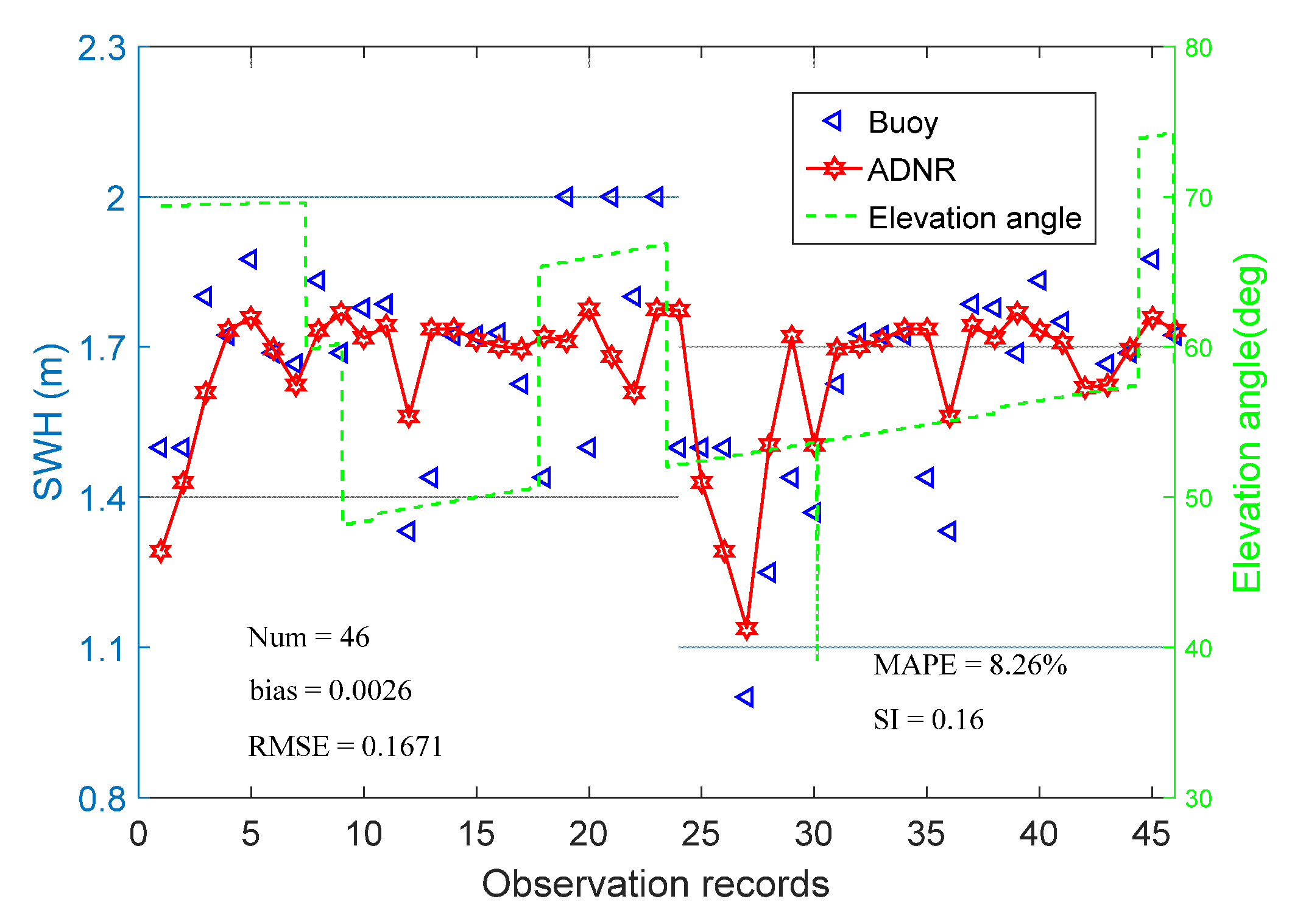
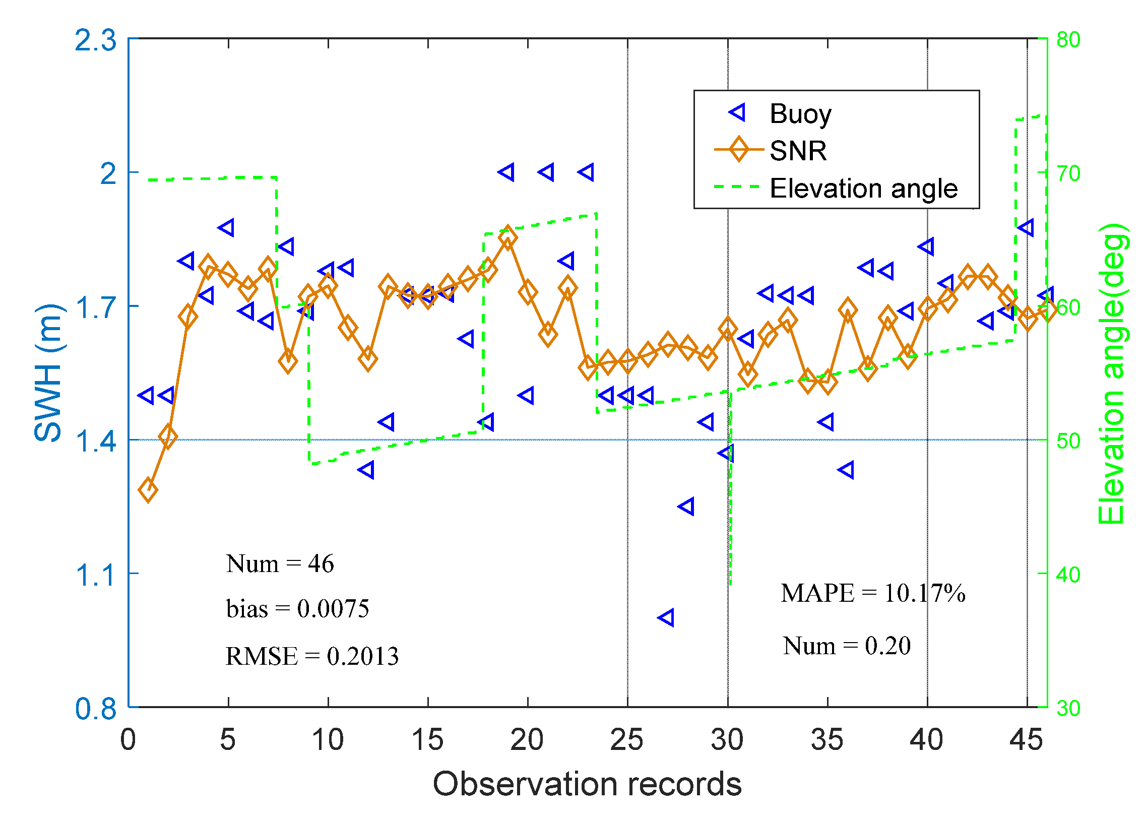
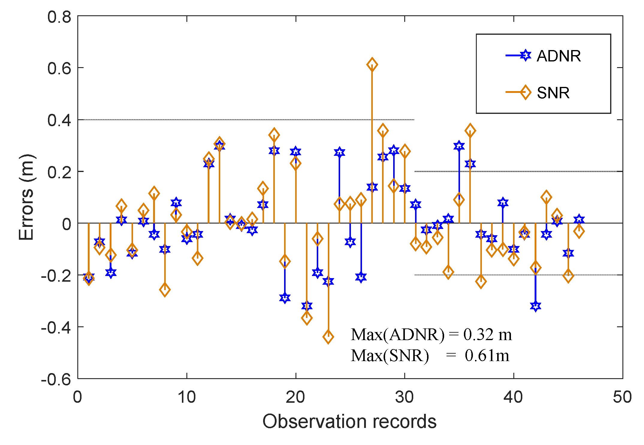
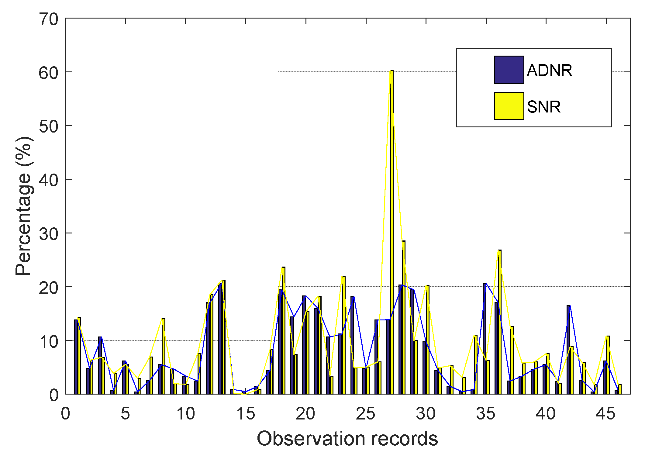
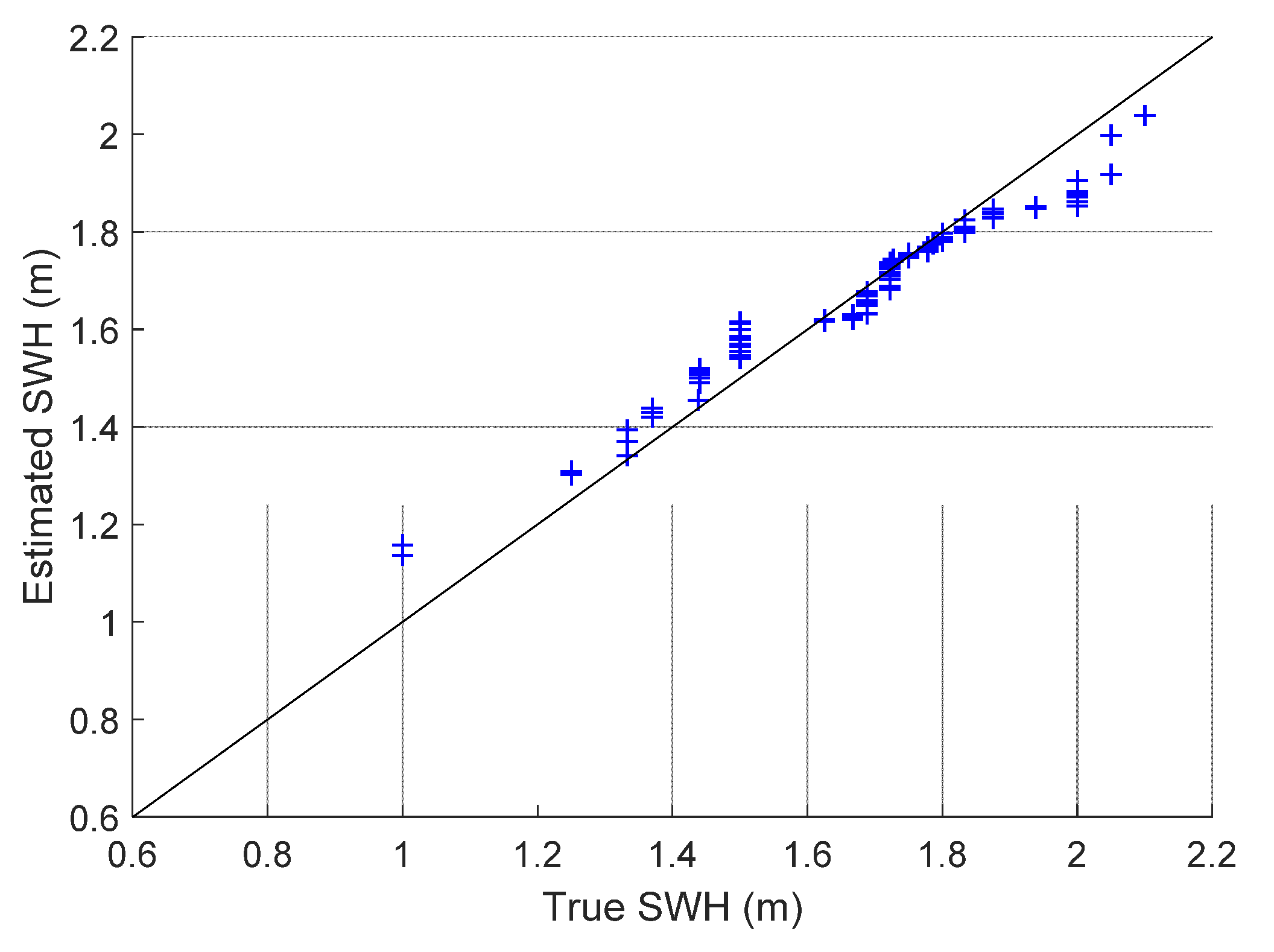
3.2. SWH Retrieval Results and Discussion

This subsection presents the experimental results and analyzes and discusses the proposed SWH retrieval algorithm.

Figure 6 presents the SWHs estimated by the proposed algorithm (denoted ADNR in the figure), and Figure 7 shows the results of the traditional SNR algorithm. In both plots, the changes of satellite elevation angles are plotted and the true SWHs are displayed for comparison. The proposed method better estimated the true data than the traditional method because it introduces the elevation angle of a second satellite to reduce the fluctuation difference among the results obtained from different elevation angles. The RMSE of the proposed algorithm was 0.1671 m, 17.00% lower than that of the traditional SNR algorithm. Furthermore, the proposed algorithm has a small scatter index of 0.16, versus 0.20 in the traditional SNR method. Figure 8 and Figure 9 compare the deviation fluctuations of the two algorithms. In each plot, the results obtained with the proposed algorithm lie closer to the y = 0 line than those of the traditional algorithm. The biases of the proposed algorithms and traditional SNR algorithms were 0.0026 m and 0.0075 m, respectively. The maximum error was 0.32 m in the proposed algorithm, versus 0.61 m in the traditional SNR method.

Meanwhile, the MAPEs of the proposed ADNR and traditional SNR algorithms were 8.26% and 10.17%, respectively, and their maximum percentage errors were 20.63% and 60.22%, respectively. However, we noticed that some of the percentage errors of the ADNR method were larger than those of the SNR method in Figure 9. It was mainly because the algorithm in this study focused on reflecting the fluctuation of true values to a greater extent during the entire estimation process (as shown in Figure 6), and a small number of individual values would be not as good as the SNR algorithm in an actual calculation, but generally reduce the mean error and maximum error. Therefore, the utilization of multi-satellite DDMs can improve the accuracy of SWH estimation. Figure 10 is a scatter plot of the SWH retrieved by ADNR versus the true SWH. Figure 11 is a Q-Q plot for the data in Figure 10. Most of the scattered points fell near the straight line. Although, there was still a gap compared with the ideal effect, and the model could be developed in further experiments.

4. Conclusions

Detecting the ocean-state information is important for marine navigation, marine disaster warnings, ocean-going, and polar exploration. An important indicator of the sea-state is the SWH. This study established an SWH retrieval algorithm using DDMs from multi-satellite observations. This approach constructs the offset correction from multiple satellite elevation angles, and improves the calculation method of SNR suitable for GNSS-R. The feasibility of this algorithm for GNSS-R estimation was confirmed in validation experiments. For comparison, we also acquired the instantaneous SWH measurements provided by the Datawell DWR-MkIII buoy. As the performance measures, we chose the bias, RMSE, MAPE, and SI. All the performance measures were lower in the proposed algorithm than in the SNR-based traditional algorithm. We thus confirmed that acquiring the multi-satellite DDMs improves the accuracy of SWH estimation.

In future experiments, we will explore researches of SWH estimation under higher sea-states to further improve the retrieval accuracy. Ultimately, research will be expected to provide services for sea-state perception and ocean observations, along with guarantees for navigation safety.

References

1. Bao, Q.; Lin, M.; Zhang, Y.; Dong, X.; Lang, S.; Gong, P. Ocean Surface Current Inversion Method for a Doppler Scatterometer. IEEE Trans. Geosci. Remote Sens. 2017, 55, 6505–6516. [Google Scholar] [CrossRef]
2. Wan, J.; Guo, W.; Zhao, F.; Wang, C. HY-2A Altimeter Time Tag Bias Estimation Using Reconstructive Transponder. IEEE Geosci. Remote Sens. Lett. 2015, 12, 1431–1435. [Google Scholar] [CrossRef]
3. Pires, N.; Fernandes, M.J.; Gommenginger, C.; Scharroo, R. Improved Sea State Bias Estimation for Altimeter Reference Missions with Altimeter-Only Three-Parameter Models. IEEE Trans. Geosci. Remote Sens. 2018, 57, 1448–1462. [Google Scholar] [CrossRef]
4. Wu, K.; Li, X.-M.; Huang, B. Retrieval of Ocean Wave Heights from Spaceborne SAR in the Arctic Ocean with a Neural Network. J. Geophys. Res. Oceans 2021, 126, e2020JC016946. [Google Scholar] [CrossRef]
5. Rodger, M.; Guida, R. Classification-Aided SAR and AIS Data Fusion for Space-Based Maritime Surveillance. Remote Sens. 2020, 13, 104. [Google Scholar] [CrossRef]
6. Angnuureng, D.B.; Jayson-Quashigah, P.-N.; Almar, R.; Stieglitz, T.C.; Anthony, E.J.; Aheto, D.W.; Appeaning Addo, K. Application of Shore-Based Video and Unmanned Aerial Vehicles (Drones): Complementary Tools for Beach Studies. Remote Sens. 2020, 12, 394. [Google Scholar] [CrossRef] [Green Version]
7. Lowe, M.K.; Adnan, F.A.F.; Hamylton, S.M.; Carvalho, R.C.; Woodroffe, C.D. Assessing Reef-Island Shoreline Change Using UAV-Derived Orthomosaics and Digital Surface Models. Drones 2019, 3, 44. [Google Scholar] [CrossRef] [Green Version]
8. Specht, C.; Lewicka, O.; Specht, M.; Dąbrowski, P.; Burdziakowski, P. Methodology for Carrying out Measurements of the Tombolo Geomorphic Landform Using Unmanned Aerial and Surface Vehicles near Sopot Pier, Poland. J. Mar. Sci. Eng. 2020, 8, 384. [Google Scholar] [CrossRef]
9. Zavorotny, V.U.; Voronovich, A.G. Scattering of GPS Signals from the Ocean with Wind Remote Sensing Application. IEEE Trans. Geosci. Remote Sens. 2000, 38, 951–964. [Google Scholar] [CrossRef] [Green Version]
10. Zavorotny, V.U.; Voronovich, A.G. Recent Progress on Forward Scattering Modeling for GNSS Reflectometry. In Proceedings of the 2014 IEEE Geoscience and Remote Sensing Symposium, Quebec City, QC, Canada, 13–18 July 2014; pp. 3814–3817. [Google Scholar]
11. Yan, Q.; Huang, W.; Foti, G. Quantification of the Relationship Between Sea Surface Roughness and the Size of the Glistening Zone for GNSS-R. IEEE Geosci. Remote Sens. Lett. 2017, 15, 237–241. [Google Scholar] [CrossRef]
12. Slater, L.B. From Minitrack to NAVSTAR: The Early Development of the Global Positioning System, 1955–1975. In Proceedings of the 2011 IEEE MTT-S International Microwave Symposium, Baltimore, MD, USA, 5–10 June 2011; pp. 1–4. [Google Scholar]
13. Baburov, V.I.; Ivantsevich, N.V.; Sauta, O.I. GLONASS Technologies for Controlling the Fields of Short-Range Navigation and Landing Systems. In Proceedings of the 24th Saint Petersburg International Conference on Integrated Navigation Systems (ICINS), St. Petersburg, Russia, 29–31 May 2017; pp. 1–4. [Google Scholar]
14. Bedrich, S.; Bauch, A.; Laverty, J.; Moudrak, A.; Schafer, W. Design of the Galileo Precise Time Facility (PTF). In Proceedings of the 18th European Frequency and Time Forum, Guildford, UK, 5–7 April 2004; Volume 2004, pp. 476–483. [Google Scholar]
15. Wang, F.; Zhang, B.; Yang, D.; Li, W.; Zhu, Y. Sea-State Observation Using Reflected BeiDou GEO Signals in Frequency Domain. IEEE Geosci. Remote Sens. Lett. 2016, 13, 1656–1660. [Google Scholar] [CrossRef]
16. Martin-Neira, M. A Passive Reflectometry and Interferometry System (PARIS): Application to Ocean Altimetry. ESA J. 1993, 17, 331–335. [Google Scholar]
17. Wang, F.; Yang, D.; Li, W.; Yang, W. On-Ground Retracking to Correct Distorted Waveform in Spaceborne Global Navigation Satellite System-Reflectometry. Remote Sens. 2017, 9, 643. [Google Scholar] [CrossRef] [Green Version]
18. Park, H.; Camps, A.; Pascual, D.; Kang, Y.; Onrubia, R.; Querol, J.; Alonso-Arroyo, A. A Generic level 1 Simulator for Spaceborne GNSS-R Missions and Application to GEROS-ISS Ocean Reflectometry. IEEE J. Sel. Top. Appl. Earth Obs. Remote Sens. 2017, 10, 4645–4659. [Google Scholar] [CrossRef] [Green Version]
19. Unwin, M.; Jales, P.; Tye, J.; Gommenginger, C.; Foti, G.; Rosello, J. Spaceborne GNSS-Reflectometry on TechDemoSat-1: Early Mission Operations and Exploitation. IEEE J. Sel. Top. Appl. Earth Obs. Remote Sens. 2016, 9, 4525–4539. [Google Scholar] [CrossRef]
20. Clarizia, M.P.; Ruf, C.S. Statistical Derivation of Wind Speeds from CYGNSS Data. IEEE Trans. Geosci. Remote Sens. 2020, 58, 3955–3964. [Google Scholar] [CrossRef]
21. Gleason, S.; Johnson, J.; Ruf, C.; Bussy-Virat, C. Characterizing Background Signals and Noise in Spaceborne GNSS Reflection Ocean Observations. IEEE Geosci. Remote Sens. Lett. 2020, 17, 587–591. [Google Scholar] [CrossRef]
22. Li, W.; Cardellach, E.; Fabra, F.; Ribó, S.; Rius, A. Effects of PRN-Dependent ACF Deviations on GNSS-R Wind Speed Retrieval. IEEE Geosci. Remote Sens. Lett. 2019, 16, 327–331. [Google Scholar] [CrossRef]
23. Wang, F.; Yang, D.; Yang, L. Feasibility of Wind Direction Observation Using Low-Altitude Global Navigation Satellite System-Reflectometry. IEEE J. Sel. Top. Appl. Earth Obs. Remote Sens. 2018, 11, 5063–5075. [Google Scholar] [CrossRef]
24. Alonso-Arroyo, A.; Camps, A.; Park, H.; Pascual, D.; Onrubia, R.; Martín, F. Retrieval of Significant Wave Height and Mean Sea Surface Level Using the GNSS-R Interference Pattern Technique: Results from a Three-Month Field Campaign. IEEE Trans. Geosci. Remote Sens. 2015, 53, 3198–3209. [Google Scholar] [CrossRef] [Green Version]
25. Peng, Q.; Jin, S. Significant Wave Height Estimation from Space-Borne Cyclone-GNSS Reflectometry. Remote Sens. 2019, 11, 584. [Google Scholar] [CrossRef] [Green Version]
26. Yan, Q.; Huang, W. Sea Ice Sensing from GNSS-R Data Using Convolutional Neural Networks. IEEE Geosci. Remote Sens. Lett. 2018, 15, 1510–1514. [Google Scholar] [CrossRef]
27. Gao, F.; Xu, T.; Meng, X.; Wang, N.; He, Y.; Ning, B. A Coastal Experiment for GNSS-R Code-Level Altimetry Using BDS-3 New Civil Signals. Remote Sens. 2021, 13, 1378. [Google Scholar] [CrossRef]
28. Chew, C.C.; Small, E.E.; Larson, K.M.; Zavorotny, V.U. Effects of Near-Surface Soil Moisture on GPS SNR Data: Development of a Retrieval Algorithm for Soil Moisture. IEEE Trans. Geosci. Remote Sens. 2014, 52, 537–543. [Google Scholar] [CrossRef]
29. Roggenbuck, O.; Reinking, J.; Lambertus, T. Determination of Significant Wave Heights Using Damping Coefficients of Attenuated GNSS SNR Data from Static and Kinematic Observations. Remote Sens. 2019, 11, 409. [Google Scholar] [CrossRef] [Green Version]
30. Soulat, F.; Caparrini, M.; Germain, O.; Lopez-Dekker, P.; Taani, M.; Ruffini, G. Sea State Monitoring Using Coastal GNSS-R. Geophys. Res. Lett. 2004, 31. [Google Scholar] [CrossRef] [Green Version]
31. Caparrini, M.; Egido, A.; Soulat, F.; Germain, O.; Farres, E.; Dunne, S.; Ruffini, G. Oceanpal: Monitoring Sea State with a GNSS-R Coastal Instrument. In Proceedings of the International Geoscience and Remote Sensing Symposium, Barcelona, Spain, 23–28 July 2007; pp. 5080–5083. [Google Scholar]
32. Shah, R.; Garrison, J.L. Application of the ICF Coherence Time Method for Ocean Remote Sensing Using Digital Communication Satellite Signals. IEEE J. Sel. Top. Appl. Earth Obs. Remote Sens. 2014, 7, 1584–1591. [Google Scholar] [CrossRef]
33. Clarizia, M.P.; Ruf, C.S.; Jales, P.; Gommenginger, C. Spaceborne GNSS-R Minimum Variance Wind Speed Estimator. IEEE Trans. Geosci. Remote Sens. 2014, 52, 6829–6843. [Google Scholar] [CrossRef]
34. Zhang, J.; Li, J. Development and Application of Big Data in the Field of Satellite Navigation. Wirel. Commun. Mob. Comput. 2021, 2021, 8850350. [Google Scholar] [CrossRef]
Figure 1. Geometry of GNSS-R.
Remotesensing 13 04806 g001
Figure 2. Relationship between satellite elevation angle and ADNR at a significant wave height of 2 m.
Remotesensing 13 04806 g002
Figure 3. Procedure of the proposed algorithm.
Remotesensing 13 04806 g003
Figure 4. GNSS-R installation, including the antennas and receiver. The RHCP (right hand circularly polarized) antenna and LHCP (left hand circularly polarized) antenna were installed on a bracket and were connected to the receiver by two RF cables. The right part is a view of Datawell DWR-MkIII.
Remotesensing 13 04806 g004
Figure 5. Location of the GNSS-R experiments (Dalian Lvshun, east China).
Remotesensing 13 04806 g005
Figure 6. Retrieval results of the proposed algorithm. The gap between two observations is 30 min.
Remotesensing 13 04806 g006
Figure 7. Retrieval results of the traditional algorithm.
Remotesensing 13 04806 g007
Figure 8. Error fluctuation in the two algorithms.
Remotesensing 13 04806 g008
Figure 9. Percentage error fluctuation in the two algorithms. Blue and yellow represent the proposed algorithm (ADNR) and SNR algorithm, respectively.
Remotesensing 13 04806 g009
Figure 10. GNSS-R-retrieved SWH versus true SWH.
Remotesensing 13 04806 g010
Figure 11. Q-Q plot for GNSS-R-retrieved SWH versus true SWH.
Remotesensing 13 04806 g011
Publisher’s Note: MDPI stays neutral with regard to jurisdictional claims in published maps and institutional affiliations.