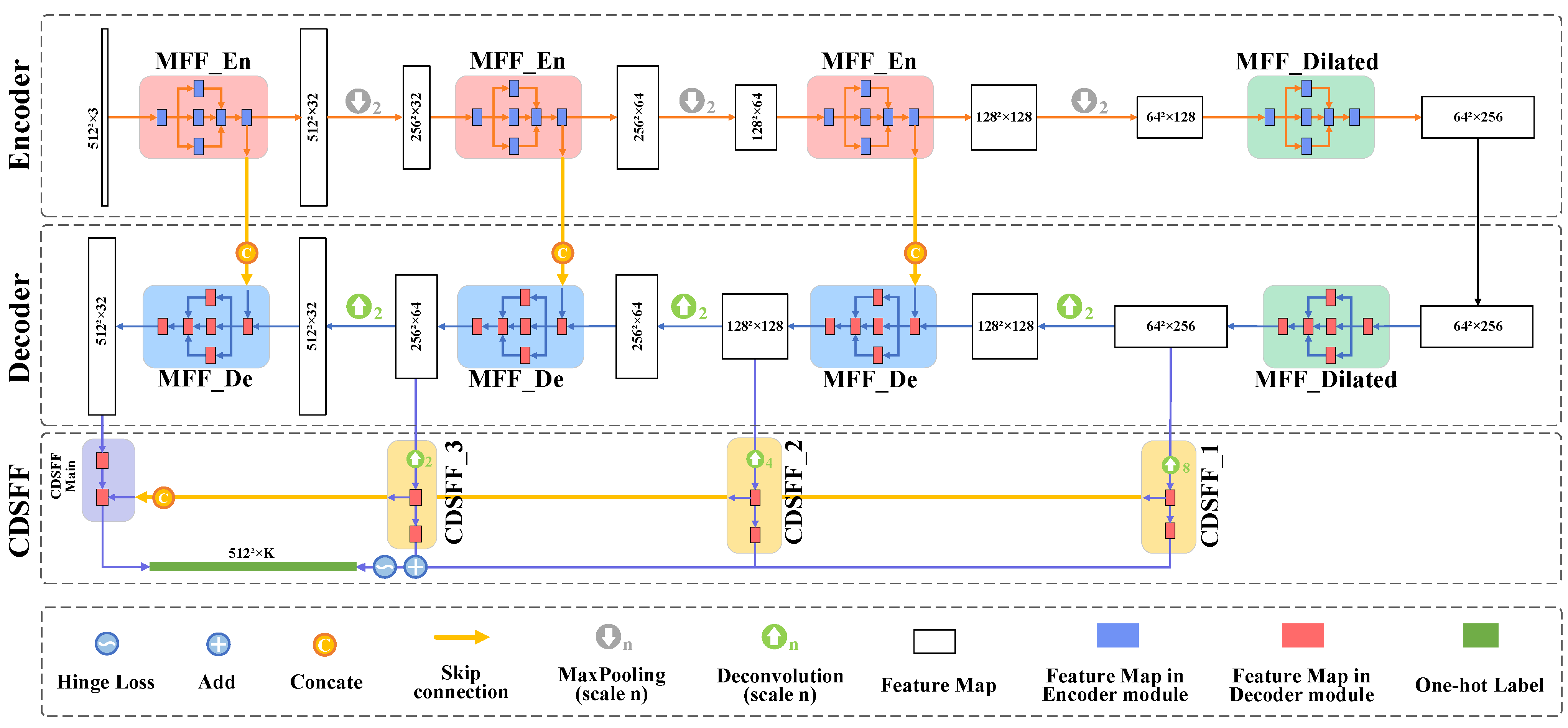
Article

Controllably Deep Supervision and Multi-Scale Feature Fusion Network for Cloud and Snow Detection Based on Medium- and High-Resolution Imagery Dataset

1
School of Geosciences, Yangtze University, Wuhan 430100, China
2
Beijing Key Laboratory of Urban Spatial Information Engineering, Beijing Institute of Surveying and Mapping, Beijing 100045, China
3
Hunan Provincial Key Laboratory of Geo-Information Engineering in Surveying, Mapping and Remote Sensing, Hunan University of Science and Technology, Xiangtan 411201, China
4
School of Computer Science, Hubei University of Technology, Wuhan 430068, China
*
Author to whom correspondence should be addressed.
Remote Sens. 2021, 13(23), 4805; https://doi.org/10.3390/rs13234805
Submission received: 29 October 2021 / Revised: 22 November 2021 / Accepted: 24 November 2021 / Published: 26 November 2021
(This article belongs to the Special Issue Deep Learning-Based Cloud Detection for Remote Sensing Images)

Abstract

:
Clouds and snow in remote sensing imageries cover underlying surface information, reducing image availability. Moreover, they interact with each other, decreasing the cloud and snow detection accuracy. In this study, we propose a convolutional neural network for cloud and snow detection, named the cloud and snow detection network (CSD-Net). It incorporates the multi-scale feature fusion module (MFF) and the controllably deep supervision and feature fusion structure (CDSFF). MFF can capture and aggregate features at various scales, ensuring that the extracted high-level semantic features of clouds and snow are more distinctive. CDSFF can provide a deeply supervised mechanism with hinge loss and combine information from adjacent layers to gain more representative features. It ensures the gradient flow is more oriented and error-less, while retaining more effective information. Additionally, a high-resolution cloud and snow dataset based on WorldView2 (CSWV) was created and released. This dataset meets the training requirements of deep learning methods for clouds and snow in high-resolution remote sensing images. Based on the datasets with varied resolutions, CSD-Net is compared to eight state-of-the-art deep learning methods. The experiment results indicate that CSD-Net has an excellent detection accuracy and efficiency. Specifically, the mean intersection over the union (MIoU) of CSD-Net is the highest in the corresponding experiment. Furthermore, the number of parameters in our proposed network is just 7.61 million, which is the lowest of the tested methods. It only has 88.06 GFLOPs of floating point operations, which is less than the U-Net, DeepLabV3+, PSPNet, SegNet-Modified, MSCFF, and GeoInfoNet. Meanwhile, CSWV has a higher annotation quality since the same method can obtain a greater accuracy on it.

1. Introduction

Long-term Earth observation permits remote sensing satellites to capture and characterize surface information [1,2], which is significant in Earth science, agriculture, forestry, hydrology, climate, and the environment [3]. However, every year, about 66 percent of the surface is covered by clouds [4]. More than 30 percent of that is covered by snow seasonally, and 10% is permanently covered by snow [5]. Satellite images covered with clouds and snow have a significant effect on Earth observation. On the one hand, clouds and snow can blur or even occlude ground objects, severely limiting the application of optical satellite data [6]. On the other hand, because snow and clouds have similar shallow features, they are difficult to distinguish from each other in cloud detection [7] or snow mapping [8]. As a result, accurate cloud and snow detection is necessary and meaningful in most remote sensing applications.
Over the years, many cloud and/or snow detection methods have been proposed. These methods can be categorized into rule-based algorithms [7,9,10,11], time difference-based algorithms [12,13,14], and machine learning algorithms [15,16,17,18,19,20,21]. First, rule-based algorithms usually analyze the differences in electromagnetic wave reflection or radiation characteristics between clouds, snow, and other objects. These differences are then combined with fixed or adaptive threshold methods to detect clouds and/or snow, such as the automated cloud cover assessment algorithm (ACCA) [10], the normalized difference snow index (NDSI) [7], the Fmask [9], and the snow detection decision tree algorithm [11]. Among them, the Fmask is frequently used to compare with the new approach since it is the classic and outstanding cloud, snow, and cloud shadow segmentation method. Meanwhile, the snow detection decision tree algorithm is a unique method for detecting shallow wet snow using brightness temperature characteristics. However, these methods only consider low-level spectral and spatial features and depend too heavily on shortwave-infrared and thermal bands [12]. Furthermore, they are overly susceptible to differences in sensor models and lack the adaptation capacity to different sensors [13]. As a result, the detection results of rule-based methods are not accurate enough [21,22], and their application is constrained. Second, time difference-based algorithms (also known as multi-temporal algorithms) exploit the dynamic properties of the clouds and snow. Therefore, the areas exhibiting significant reflectance fluctuations between multi-temporal images will be detected as clouds or snow, such as Tmask [23], CS [14], ATSA [24], and the multi-temporal cloud and snow detection algorithm [12]. Due to the high cost of intensive time-stacks image collection [13], the poor detection of permanent snow-covered areas [23], and unpredictable surface landscape changes, the operation of these methods is restricted.
Machine learning algorithms detect clouds and snow using trained classifiers such as the Support Vector Machine [15,16,17], Random Forest [19], Classical Bayes [25], and Neural Networks [18]. As higher-level spatial features such as the texture, shape, and contour of clouds and snow are utilized in these approaches, the detection accuracy can be increased. Nonetheless, because of the constraints of classifier performance and the trainable parameter capacity, several machine learning techniques have been proven to be inferior to the Fmask in complex tasks [9,22]. As a branch of machine learning, deep learning has made significant progress in recent years [21,26]. Its precision, generalization ability, and inference speed have all been improved. Meanwhile, convolutional neural networks (CNNs) have been used in a slew of cloud and/or snow detection studies, with encouraging results. These methods concentrate on two aspects: quick response and execution precision.
In terms of methods for a quick response, the lightweight RS-Net [21] and U-Net-modified [13] give significant attention to the fast-reasoning capability of the model, while ensuring accuracy. Both models employed the U-Net [27] as the backbone and halved the depth of the feature maps. Thus, their computational cost and number of parameters were reduced. On a Landsat8 product, the average cloud masking time of RS-Net has been decreased to roughly 18 s. Simultaneously, the reasoning time of the U-Net-modified model is almost 1/60 of the Fmask. These two models also outperform the Fmask in terms of detection accuracy.
The contribution to enhancing detection accuracy mainly focuses on incorporating complex components or changing the network structure. On the one hand, some methods introduce an optimized component into the network. In [28], the authors added the multi-level semantics information fusion module to the VGG [29] to improve the cloud and snow detection accuracy. MFFSNet [20] took ResNet101 as the main structure and introduced an enhanced pyramid pooling module [30]. It could obtain the relationship context of the cloud and shadow and combine the various levels of abstract features and spatial information. The performance of the network was superior to that of PSPNet and DeepLab. MF-CNN [31] incorporated a multi-scale module that could aggregate abstract features of various scales. Meanwhile, the network fused low-level spatial and high-level semantic features to precisely separate thick and thin clouds. On the other hand, some approaches focus on modifying the feature extractors in the encoder and decoder. Based on FCN [32], the Cloud-Net [33] meticulously designed cloud blocks to extract and integrate local and global semantic cloud features. It promoted the network to achieve high-level precision. MSCFF [34] took the improved Resnet50 [35] as its backbone. Before a unified output, it fused several levels of feature maps in the decoding part. This system promoted the fusion of multi-level advanced semantic information. From that, the MSCFF showed excellent precision on a variety of satellite datasets.
Although the preceding deep learning methods have improved the efficiency and accuracy of cloud and/or snow detection, the majority of them are designed and validated based on medium-resolution datasets with a wide range of bands. However, high-resolution (resolution within 10 m) satellite image applications have grown extensively in recent years. The need for cloud and snow detection from high-resolution remote sensing images has surged. Furthermore, the number of bands available in high-resolution images is limited. Therefore, the applicability of the above methods to high-resolution remote sensing images with limited accessible channels needs to be demonstrated further. Moreover, deep learning methods that excessively emphasize execution efficiencies, such as RS-Net and U-Net-modified, are insufficient in terms of accuracy [36,37], whereas the networks that prioritize accuracy, such as MSCFF, MFFSNet, and Cloud-Net, dramatically increase the computation cost as the number of parameters increases.
Inspired by the above issues, this research presents a convolutional neural network for detecting clouds and snow. It applies to medium- and high-resolution remote sensing images with visible bands. More importantly, it considers both reasoning speed and segmentation precision. Additionally, a high-resolution cloud and snow dataset was published. The following are the more specific innovations:
(1)
A cloud and snow detection network (CSD-Net) is proposed to generate cloud and snow masks according to the input satellite imageries. The network can robustly achieve a satisfactory detection accuracy and speed on medium-resolution and high-resolution remote sensing images with only RGB channels, due to two innovative components, including the multi-scale feature fusion module (MFF) and the controllably deep supervision and feature fusion structure (CDSFF).
(2)
The decoder and encoder of the network are driven by the MFF with parallel channels, so that, throughout the shallow and deep layers of the network, CSD-Net may gain low-level features with various granularities and advanced features with varying scales, respectively. This allows the network to better discriminate between clouds and snow objects, owing to the more comprehensive features obtained.
(3)
The CDSFF is deployed in the decoding part to establish a deep supervision structure with a tunable loss mechanism. It encourages the network to securely learn more representative features and improve the propagation of gradient flows within the network. Additionally, it fuses local and global features, enriching the captured features of clouds and snow.
(4)
An open-source cloud and snow dataset based on WorldView2 (CSWV) h tagged manually. It contains two sub-datasets: the submeter-level high-resolution cloud and snow dataset (CSWV_S6) comprises six scenes with a resolution of 0.5 m; the meter-level high-resolution cloud and snow dataset (CSWV_M21) includes 21 resampled scenes with a resolution of 1–10 m.
The rest of the manuscript is organized as follows: Section 2 delves deeper into the proposed CSD-Net. In Section 3, the experimental dataset is introduced. Section 4 explores the experimental setup and results in detail. Section 5 discusses the details of the method and dataset. In Section 6, we draw a summary of all the work in this paper.

2. Proposed Method

In this section, we provided a quick review of CSD-Net. Then, two key components, the multi-scale feature fusion module (MFF), and the controllably deep supervision and feature fusion structure (CDSFF) are described in detail.

2.1. Overview of CSD-Net

Figure 1 depicts the architecture of CSD-Net. It receives cloud and snow remote sensing images, extracts and exploits the multi-level features in an end-to-end manner, and then generates cloud and snow masks. The specific structures of this network are listed as follows: First, after stacking numerous times, MFF ran through the encoder and decoder of the network. This component extracted and aggregated multi-scale cloud and snow features. Second, CDSFF was distributed in the decoding part. It added a supervision mechanism with hinge loss to the middle layer and fused the available features of adjacent layers in the decoder. Third, skip connections were established between the equivalent feature maps of the encoder and decoder. These structures compensated for the loss of information during the max-pooling and convolution processes by propagating the lower-level features and location information to the depths of the network. Finally, the depth of the network feature maps was substantially decreased for reducing the number of parameters, training time, and the risk of overfitting.

2.2. CSD-Net: Multi-Scale Feature Fusion Module (MFF)

The thin clouds and the underlying surface can be easily confused, as are the nearly melted snow and the surrounding bare land. In addition, the cloud and snow features are similar in spectral features. Therefore, the existing methods are prone to generating more erroneous and missing detection results. In our research, we designed the MFF module to extract features with different granularities to aggregate richer multi-scale features to minimize the impact of similar objects.
In MFF, the basic module containing a convolution layer, a batch normalization layer [38], and a rectified linear unit (ReLU) activation layer was named the CBR block. In contrast, another basic module that lacks the batch normalization layer was named the CR block. The batch normalization layers made the network easier to train and fit [38]. Simultaneously, ReLU activation function layers could incorporate additional nonlinear mapping to boost the generalization capability of the network. Figure 2 describes the detailed process of constructing MFF. First, MFF used the 3 × 3 CBR basic module to change the number of the feature map channels. Second, the 1 × 1, 3 × 3, and double 3 × 3 CR basic modules were stacked in parallel channels. The concatenation layer followed. Therefore, MFF could extract and fuse diverse granularity features from different ranges of domains. This structure was conducive to enhancing the links between features of different scales and capturing richer kinds of semantic information for cloud, snow, and background, resulting in the best local sparse structure in two dimensions [39]. Third, the 1 × 1 CBR basic module reduced the depth of the feature map. Then, the information was compressed, and a sparse connection in the third dimension could also be achieved. In the last step, to create the identity mapping, the residual structure [35] was introduced between the feature maps generated in the first and third steps. In summary, the network captured more abstract and discriminative semantic information after the entire MFF processing.
As the MFF location changes in the encoding and decoding parts, the insertion location of the skip connection structure and the depth of feature maps changed. All the MFF structures were fine-tuned to accommodate the changes. We referred to them as MFF_En and MFF_De to distinguish various modified components, as illustrated in Figure 3. In addition, all 3 × 3 convolutions in the final MFF_En and the first MFF_De were converted to dilated convolutions and the skip connections were canceled. We further named this kind of MFF as MFF_Dilated. Their dilation rate was dynamically allocated to apply to image datasets with varied resolutions. This improvement helped to boost the receptive field, allowing the network to retain more meaningful information. The MFF underwent several modifications and was then added to the network, as shown in Figure 1.

2.3. CSD-Net: Controllably Deep Supervision and Feature Fusion Structure (CDSFF)

Even though MFF improves the discrimination of the features captured by CSD-Net, it is difficult for the middle layer to learn directly and transparently during the training process. Additionally, as the depth of the network grows, gradient vanishing or explosions may occur [40,41,42]. As a result, we designed a controllably deep supervision and feature fusion structure (CDSFF) as an early additional constraint to add to the decoding layer.
As shown in Figure 1, the feature maps in the decoder processed by MFF built a deeply supervised mechanism through CDSFF. Figure 4 displays that the deconvolution layer was initially employed in CDSFF to rebuild the feature map, returning the input feature map to its original size and reducing the number of channels. Then, the feature map was fed to the main output structure, which fused features at several levels to gather better local and global context information about clouds and snow. Finally, the 1 × 1 convolution and the Softmax activation function mapped the feature maps into the confidence measure matrices Y , which is described by Equation (1). Simultaneously, the categorical cross-entropy function was employed to evaluate the difference between the predicted values Y and actual values Y ^ , as depicted in Equation (2).
Y k = σ ( Z ) = e x p ( Z k ) i = 1 K e x p ( Z i )   , k ( 1 K ) ,
( Y ^ , Y ) = 1 h × w k = 1 K i = 1 h j = 1 w [ Y ^ k , i , j log ( Y k , i , j ) ] ,
where Y k is the confidence measure matrix of the k-th category. Z is the output of the filter/convolution kernel before the classifier. σ is the softmax activation function. K , h , and w represent the number of classifiable categories, the height, and the width of the input image, respectively. The loss function is denoted by .
Rather than the standard networks of merely providing supervision at the output layer, CDSFF installed several feature-quality feedback devices in the hidden layers, which have the potential to boost the gradient flow momentum in the shallow layers. Therefore, it increased convergence speed and provided a strong regularization to learn more powerful and representative features. Nevertheless, the resolution of the feature maps in the decoding arm (e.g., the feature map connected with CDSFF_1 in Figure 4) was too low, and these feature maps lacked sufficient fine features. Especially after attaching the CDSFF, the large-scale resolution recovery and depth reduction increased the fine information loss. It could directly impact the updating of the front-layer parameters and affect the overall network performance. Thus, different coefficients were weighted to the CDSFF associated with different level feature maps, as defined in Equation (3) and shown in Figure 4. This balanced the importance of the gradient flow in different companion output paths and suppressed backpropagation with errors.
all ( Y ^ , Y ) = ω 0 × main ( Y ^ , Y ) + i = 1 3 ω i × i ( Y ^ , Y ) ,
Furthermore, the features in low-resolution feature maps were coarse-grained and abstract. While the gradient inside the network tended to be stable in later stages of training, these feature maps were too direct to learn from the target features. It increased the chances of learning signals that were incorrect and introduced uncertainty into the network. As a result, CDSFF incorporated hinge loss [43] to safeguard network performance against this issue. Hinge loss indicated that if the loss value fell below a specific threshold, it would be set to 0. It was generally used to deal with classification techniques using support vector machines. In our research, we refined the hinge loss and applied it to CDSFF. It allowed the gradient descent algorithm to ignore the deep supervision branch losses if the sum of these losses was less than the artificial set safety factor α   (Equation (4)). This innovation prevented the gradient flow with errors in the network during the latter stage of training.
all ( Y ^ , Y ) = ω 0 × main ( Y ^ , Y ) + max ( l = 1 3 ω l × l ( Y ^ , Y ) α , 0 ) ,
To summarize, CSD-Net mapped the given image X h × w × c to the pixel level confidence map Y h × w × k and produced the cloud and snow mask. Meanwhile, the proposed modules substantially refined the detection results and minimized gradient disappearance or explosion possibilities. We validated these benefits detailed in Section 4.

3. Dataset

The datasets involved in the experiment were explained and compared in this section.

3.1. Existing Cloud and Snow Datasets

Cloud detection has made significant progress in recent years, and many relevant datasets have been generated [33,44,45,46,47,48]. However, the datasets for cloud and snow detection are rare, including Levir_CS [49] and the Landsat8 SPARCS (L8_SPARCS) [18] dataset. The details of these two datasets are as follows:
Levir_CS is a dataset dedicated to cloud and snow detection in low-resolution images. It gathers 4168 scenes from GF-1 WFV, with distinct ground cover types and climate. The original images have a spatial resolution of 16 m. However, they are 10× downsampled. Finally, 1320 × 1200 pixel-sized image blocks with a spatial resolution of 160 m are gained. Each pixel in the dataset is assigned to one of three categories: “cloud”, “snow”, and “background”. Simultaneously, metadata such as the longitude, latitude, and height are included in the dataset as well.
The L8_SPARCS dataset has 80 scenes collected by Landsat8 with a 30 m spatial resolution. Additionally, it is manually labeled with seven categories: “cloud”, “cloud shadow”, “snow/ice”, “water”, “cloud shadow on the water surface”, “flood”, and “clear sky”. As this dataset includes cloud and snow labels, it can also be trained and tested using deep learning methods for cloud and snow detection. To make the dataset suitable for the task of cloud and snow detection, only the “cloud”, “snow/ice”, and “clear sky” categories of the dataset were preserved in this experiment, and all other categories were consistently grouped into “clear sky”. In our experiment, we used visible spectral bands from the L8_SPARCS and ignored other channels.
Although the two datasets are suitable for cloud and snow detection, their resolution is only 160 m and 30 m, respectively. Thus, the existing datasets cannot meet the needs of high-resolution cloud and snow detection tasks.

3.2. CSWV Dataset

Since there is no high-resolution cloud and snow dataset, we constructed a public dataset with a 0.5–10 m spatial resolution, termed the cloud and snow dataset based on WorldView2 (CSWV). It included 27 WorldView2 images with clouds and snow, located in the North American Cordillera mountains and acquired from June 2014 to July 2016. The ground surface in these scenes was complex, including a forest, grassland, lake region, bare ground, etc. The clouds in the images varied, including cirrus, cirrocumulus, altocumulus, cumulus, and stratus clouds. Meanwhile, in the images, the snow comprised of permanent snow, stable snow, and discontinuous snow. The variety of clouds and snow increased the heterogeneity of their form, size, thickness, brightness, and texture, making the dataset more generalizable and representative.
The dataset was further divided into two subsets for assessing the performance of methods on the submeter-level and meter-level high-resolution remote sensing images. Six of the 27 scenes were left unprocessed and named the submeter-level high-resolution cloud and snow dataset (CSWV_S6), with a resolution of 0.5 m. Through resampling, the remaining 21 scenes constructed a meter-level high-resolution cloud and snow dataset (CSWV_M21), with various resolutions from 1 to 10 m.
As far as we know, CSWV is the first freely available dataset for cloud and snow detection with high-resolution remote sensing imageries. Figure 5 illustrates several CSWV_S6 and CSWV_M21 annotation examples. Simultaneously, the dataset was made available at https://github.com/zhanggb1997/CSDNet-CSWV (accessed on 24 November 2021) for free to assist other researchers in conducting relevant research.

3.3. The Comparison of the Datasets

Because we focused on cloud and snow detection applications in medium-resolution and high-resolution remote sensing images, this experiment employed the L8_SPARCS dataset and the CSWV dataset we proposed. The experimental data spanned a wide range of datasets with spatial resolutions ranging from 0.5 to 30 m, as shown in Table 1. In the datasets, CSWV_S6 had the most available pixels and the highest spatial resolution. The sub-meter high-resolution and the large number of pixels in CSWV_S6 made it more difficult to annotate, resulting in fewer scenes than in other datasets. Additionally, the statistical chart of different category proportions in the three datasets is depicted in Figure 6. It can be seen that the proportion of cloud and snow pixels in L8_SPARCS was 19.37% and 5.3%, respectively, with a 14.07% gap. Our proposed CSWV_M21 and CSWV_S6 datasets had a higher proportion of cloud and snow pixels than L8_SPARCS. Additionally, the ratio difference between the two categories was more balanced, with only 9.31% and 9.42%, respectively.

4. Experiments and Results

Ablation studies and comparison experiments in terms of the accuracy and efficiency were carried out in this section.

4.1. Experimental Setup and Details

The whole scenes in L8_SPARCS, CSWV_M21, CSWV_S6, Landsat8 Biome (Biome) [44,50], and HRC_WHU [34] were sliced into patches with 5122 pixels. Then, the clipped patches were divided into three subsets: the training set, validation set, and testing set, intended for a deep convolution neural network learning optimization, unbiased assessment, and final evaluation, respectively. Each subset assured the independence and randomness of data during the partitioning process.
Overfitting was common in the training process due to the limited number of available training data. Therefore, data augmentation was employed to enlarge the number of image blocks and corresponding labels. This process did not increase the labeling burden [51], but the robustness of the network was strengthened by learning more invariance in the data augmentation field. Since the snow and clouds had minor spectral differences and complex natural contours, the transformation augmentation approach incorporating color, contrast, and geometric aspects was abandoned. Therefore, rotation operations were employed in L8_SPARCS, CSWV_M21, and CSWV_S6 only three times. As a result, the enlarged dataset was four times the original dataset. Because there was a clear gap in the number of image patches in the three datasets, the fixed proportion of the train, validation, and test subsets introduced fortuity to the network prediction results. Therefore, the proportions of subsets differed between various datasets. Table 2 gives a detailed description of the experimental settings.
All of the experiments in this study were carried out on a computer running Windows 10 64-bit. The AMD Ryzen5 5600X 6-Core Processor, 32GB of memory, 1TB SSD, 4TB mechanical hard disk, and NVIDIA GeForce RTX 3090 graphics card with 24GB of video RAM were all included in the device. We next built a deep learning environment employing Python3.8 [52], PyTorch1.8.0 [53], and CUDA11.1 [54]. All of the network models in the experiment were implemented using the above hardware and software environment. The random seed was set to 0 and served as the initialization weight of the network. The adaptive motion estimation (Adam) optimizer was applied for gradient descent during the training process. The loss function was the categorical cross-entropy function, with the learning rate set at 0.0001. Then, the epochs were set to 80 or 120, and the batch size was 8. In the experiment, the automatic mixed precision (AMP) of PyTorch [53] and the gradient scaling mode were both enabled. Therefore, each operation in training could automatically find the best match between the float16 and float32 data types and reduce memory occupancy. The benchmark strategy was also activated, which could encourage cuDNN [55] to select the most efficient algorithm for the current convolution task to accelerate training.

4.2. Evaluation Metrics

The overall accuracy (OA), mean intersection over union (MIoU), Kappa, F1-score (F1), recall (Rc), and precision (Pc) were used as evaluation metrics in our experiment to assess the accuracy of cloud and snow detection. It should be noted that for the controversial F1, Rc, and Pc, this paper adopted the calculation method proposed in [56]. We labeled them as Macro-Rc, Macro-Pc, and Macro-F1, respectively. The following formulas show the metrics definition:
OA = Po = i = 1 c TP i t ,
MIoU = i = 1 c IoU i c ,
Pe = i = 1 c P i × ( TP i + FN i ) + N i × ( TN i + FP i ) t 2 ,
Kappa = Po Pe 1 Pe ,
Macro F 1 = i = 1 c F 1 c ,
Macro Rc = i = 1 c Rc i c ,
Macro Pc = i = 1 c Pc i c ,
where i stands for the i-th category, c is the total number of categories, and t denotes the total number of pixels.

4.3. Ablation Experiments

Various feature extractors or technology components were deployed to form the new networks. These networks were trained and tested on the enhanced CSWV_S6 dataset to evaluate how different modules affected the detection accuracy, space complexity, and time complexity. All of these studies were intended to verify the rationality and efficacy of our suggested components in various aspects. The setup details for eight networks (a)–(h) used to execute ablative experiments are shown in Table 3. In the experiments, the network structure was modified, or new components were introduced, while the rest of the setup stayed unchanged.
Network (a): all MFF modules in CSD-Net were replaced by two serial CBR basic modules with 3 × 3 filters, and the CDSFF in CSD-Net was also removed. The rest of the structures remained unchanged. The processed network was used as the backbone for the other improved components.
Network (b): MFF_En, MFF_De, and MFF_Dilated are inserted into matching locations in the network (as defined in Section 2.2 and Figure 1). The effect of MFF on the network performance could be determined by comparing the results of this network to those of network (a).
Network (c): the deep supervision structure (DS) was extracted after deconstructing the CDSFF. Then, the DS was combined with network (b) to construct the network (c). The experiment based on network (c) could be employed to validate the effect of the DS.
Network (d): the controllable loss mechanism (CL) was eliminated in CDSFF from a deep supervision and feature fusion structure (DSFF). Then, the DSFF was integrated into network (b). Compared to network (c), it could particularly examine the availability of the feature fusion structure (FF).
Network (e): CDSFF was deployed on the network (b) to build a full CSD-Net. This network intended to compare with network (d) and validate the efficacy brought by the controllable loss mechanism (CL).
Network (f): based on network (e), the 1 × 1 and 3 × 3 CR channels in the MFF were removed. This network was used to test the impact of a multi-channel network on the cloud and snow detection accuracy.
Networks (g) and (h): based on network (e), both networks replaced the MFF multi-channels with the Inception V1 naive module [39] and the Inception V4-A module [57], respectively. The performance difference between the traditional multi-channel modules and our well-designed MFF module were verified using these networks. Table 3 displays the quantitative evaluation results of the eight networks.
MFF showed excellent feature extraction and network optimization capabilities. Table 3 shows that, as compared to network (a), the MIoU, Macro-F1, and Kappa of network (b) rose by 2.29%, 1.33%, and 3.83%, respectively. The reason for the accuracy improvement was that MFF brought more trainable parameters and multi-scale spatial domain features to the network, which helped the network to obtain more advanced semantic information. Simultaneously, by comparing the loss curve of the validation set in Figure 7a, network (b) accelerated the gradient descent during the early training process because of the residual structure in the MFF. In brief, MFF in the network could determine significant contributions to both the detection accuracy and convergence speed. Meanwhile, removing the multi-channel from MFF reduced the potential of multi-granular feature fusion, as well as the overall performance of the network. As shown in Table 3, the MIoU, Macro-F1, and Kappa of network (f) were reduced by 2.81, 1.71, and 1.39, respectively, when compared to network (e). Moreover, network (g) results showed that when the multi-channel structure was replaced with the Inception V1 module, the complexity of the network increased, and the capacity to extract features was harmed. Especially in network (h), the detection accuracy dropped dramatically. In conclusion, our well-designed MFF was particularly effective in dealing with cloud and snow detection tasks, as seen by the comparison with other multi-channel modules.
CDSFF was also useful for increasing the network performance. Its substructure, the deep supervision structure (DS), enhanced the detection accuracy of MIoU, Macro-F1, and Kappa by 1.34%, 0.83%, and 0.62%, respectively, compared to network (b). Furthermore, because the deep supervision mechanism was incorporated into the hidden layer, the network fitting was expedited in the early training stages, as seen in Figure 7b. Although DS did not perform as well as MFF in terms of improving the accuracy and accelerating the convergence speed, the network with DS did not significantly increase the complexity of time and space. The feature fusion mechanism (FF) produced a gain in detection precision that was not obvious, but we could see that this structure improved the overfitting of the network in the latter stages, as shown in Figure 7c. Network (e), with a controllable loss mechanism (CL), outperformed network (d) by 1.64%, 0.97%, and 1.00% on MIoU, Macro-F1, and Kappa, respectively. Additionally, it also did not bring the additional computational cost and parameters of the network. However, due to the complexity of its loss curve over the validation set, we did not obtain valuable insights. After integrating the DS, FF, and CL, we could gain the CDSFF. Compared with network (b), network (e) with CDSFF could improve the feature extraction and fitting ability of the network. Meanwhile, the time and space complexity of the network did not improve significantly, as can be seen in Table 3.

4.4. Comparison with Other SOTA Methods

In this section, a series of comparisons were used to validate the performance of the proposed method. We selected three classic deep learning models: U-Net [27], PSPNet [30], and DeepLabV3+ [58] for comparison. Moreover, five semantic segmentation networks for cloud and/or snow detection were also contrasted: RS-Net [21], SegNet-Modified (after this referred to as SegNet-M) [22], MSCFF [34], GeoInfoNet [49], and CDnetV2 [37]. Eight state-of-the-art (SOTA) deep learning methods and CSD-Net were trained and predicted based on the L8_SPARCS, CSWV_M21, and CSWV_S6 datasets.

4.4.1. Accuracy Evaluation and Comparison

We calculated the quantitative accuracy of the predicted results and listed them in Table 4. The visual comparisons of the results are also presented in Figure 8, Figure 9, Figure 10, Figure 11, Figure 12 and Figure 13. Through the overall comparison, we could find that CSD-Net was far superior to the other networks, both in terms of quantitative evaluation values and subjective visual feelings. Next, we provided a more detailed comparison.
In the L8_SPARCS, the detection results of the compared methods had many low-level errors. The large scene results in Figure 8 showed that CSD-Net was extremely close to the ground truth. However, other methods had a lot of cloud detection noise in the snow area, and it was simple to mistake the clouds with the high reflection of snow. Figure 9 gives a more detailed representation of the results, revealing that U-Net, PSPNet, DeepLabV3+, RS-Net, MSCFF, GeoInfoNet, and CDnetV2 all mistook certain snow areas with evident snow characteristics for clouds. Meanwhile, SegNet-M, DeepLabV3+, U-Net, and CDnetV2 mistook vast cloud patches with fine and smooth surfaces for snow. Evidently, all the compared methods were inadequate for cloud and snow detection. According to Table 4 (a), we could see that the MIoU of these methods was significantly lower than CSD-Net. There were three main reasons for this phenomenon. First, the spatial and spectral features of cloud and snow objects were similar, making it challenging for the network to learn distinguished features from limited training samples. Second, the percentage of cloud and snow pixels in the L8_SPARCS dataset was overly imbalanced, which aggravated the learning bias of networks. Third, the compared methods had no robust feature extracting ability on tiny or sample-unbalanced datasets. As a result, during the detection phase of the competing methods, low-level errors arose. On the contrary, our proposed method had no distinct misclassification in Figure 8 and Figure 9. Moreover, Table 4 (a) shows that the MIoU, Macro-F1, Kappa, and Macro-Rc of CSD-Net were higher than the second-best MSCFF by 3.65%, 2.25%, 1.70%, and 4.85%, respectively. The reason was that CSD-Net had a modest number of parameters and benefits from MFF and CDSFF, which allowed it to have unbiased learning and prevent overfitting.
The detection results based on the CSWV_M21 scenes are depicted in Figure 10 and Figure 11. Although PSPNet and DeepLabV3+ could detect the majority of cloud and snow objects, they had many misclassifications and were unable to recover more detailed masks. Hence, the evaluation scores on MIoU for these two networks were relatively low in Table 4 (b), with only 75.59% and 69.51%. Other comparison methods were fairly accurate, but their ability to detect details was different. Figure 10 and Figure 11 showed that the bare land and cement floors with sunlight were easily identified as thin clouds in the detection results of U-Net, PSPNet, DeepLabV3+, RS-Net, GeoInfoNet, and CDnetV2. Meanwhile, some discontinuous fine cloud pixels at the border of thick clouds were overlooked and misidentified by U-Net, PSPNet, DeepLabV3+, SegNet-M, and CDnetV2. Although RS-Net, MSCFF, and GeoInfoNet can detect as many thin clouds as possible, this led to oversensitivity for the snow areas with shadows and the bright ground areas with sunlight. Moreover, there were frequent misclassifications of U-Net, DeepLabV3+, and SegNet-M detection results in the city area, as bright building roofs were misinterpreted for snow. Furthermore, all the comparison methods were challenging to identify the clouds over the snow. Because the results of the compared methods had a huge number of misclassifications, their accuracy was relatively low, as shown in Table 4 (b). Figure 10 and Figure 11 show that CSD-Net could provide satisfactory prediction results. Specifically, it could accurately identify clouds over the bright surface and retrieve more refined thin clouds. Meanwhile, it minimizes the likelihood that underlying surfaces (such as building roofs, pavements, and bare ground) are misidentified as snow. In addition, Table 4 (b) demonstrates that CSD-Net had the highest values on MIoU and Macro-F1, which were 87.05% and 93.01%, respectively. These precision advantages benefited from the unique structure of CSD-Net, which could be summarized as follows. First, the skip connection structure in CSD-Net delivered more position and appearance information to the deeper network. Meanwhile, the CDSFF aggregated the feature maps from the different tiers of the decoder. Both structures were capable of retaining more refined features of thin clouds and snow patches. Second, the MFF constantly collected and combined the multi-scale information from the feature domain, allowing the network to better differentiate the distinct objects in cloud-snow coexistence areas and complex urban scenes.
The visual comparison of CSWV_S6 test results is listed in Figure 12 and Figure 13. In comparison, the detection results of the compared methods did not have substantial errors on the cloud edge and only had some small detection noises. However, more obvious issues could be found in the interior of the clouds and the shadow regions. Cloud centers with high reflectivity were prone to misclassification by comparison methods. Moreover, the comparison methods also easily misidentified the snow regions and bare land covered by the shadows as the clouds. This was because, as the spatial resolution increased, the amount of information that could be conveyed in the small-sized image block decreased. It was more difficult for networks to capture distinguishing features from image blocks with constrained information. In comparison, our method performed better at detecting delicate clouds and eliminating the above issues as much as possible. In addition, U-Net, DeepLabV3+, RS-Net, SegNet-M, MSCFF, and GeoInfoNet were prone to misidentifying high-reflectivity structures as snow. The reason was that the strong reflectivity on the tops of some buildings in the high-resolution imageries was comparable to snow. Meanwhile, our dataset did not contain many urban scenes, and these methods were incapable of robustly extracting distinguishing features from the limited samples. The MIoU and Macro-F1 of the best CSD-Net were 88.54% and 93.83%, respectively. They were 1.91% and 1.14% higher than the second-best MSCFF. The following are the facts why CSD-Net could create such precise masks. The max-pooling layer and the MFF_Dilated enabled the receptive field of the network to expand considerably. It aided the network in receiving more complete information about large-sized objects in high-resolution images. Moreover, the CDSFF caused the features in the middle layers to directly learn from ground truth, which could substantially reduce low-level misclassification in information-insufficient areas.
To summarize, CSD-Net obtained the maximum MIoU, Macro-F1, Kappa, OA, and Macro-Rc values in all datasets. The majority of the compared methods were able to generate generally satisfactory masks, but they were less precise than CSD-Net. More specifically, DeepLabV3+ performed the worst in various datasets. This may be attributed to information loss caused by its large-stride upsampling in the decoder, resulting in a decline in the detection performance. Among the deep learning algorithms appropriate for cloud and snow detection, GeoInfoNet had a relatively low reliability, because the proposition of GeoInfoNet focused on confirming network performance improvements by using geographic information rather than making significant changes to the network structure. PSPNet, U-Net, RS-Net, and SegNet-M performed moderately and differently on various datasets. To state it another way, the assessment scores of these methods may have been high in one dataset but mediocre in another, since the capacity to extract features of these methods was not robust and generalized. Despite the fact that CDnetV2 used several novel feature fusion blocks and feature guidance flows, the large-scale sampling in the decoder made it challenging to achieve fine results. The MSCFF could fuse rudimentary appearance and abstract semantic information based on the excellent feature extractor and fusion structure. These benefits ensured the accuracy of MSCFF on various datasets was always suboptimal. By contrast, our proposed method could extract most fine clouds, even over the snow. Meanwhile, the snowy places polluted by shadows and bright bare lands could be the correct classification. Moreover, our approach was not misled by buildings or exposed ground and did not misclassify them as snow or clouds. As a result, the masks generated by CSD-Net had an excellent matching effect with ground truths.
Furthermore, Equation (6) shows the MIoU was the average of the IoU for all categories. Therefore, the MIoU had a uniformity and was unable to represent the single-category detection accuracy adequately. Therefore, the intersection over union (IoU) evaluation metrics for clouds and snow were calculated and plotted in Figure 14. The IoU of cloud (IoUc) and the IoU of snow (IoUs) generated by CSD-Net on the three datasets were the greatest. Moreover, the difference between the IoUs and IoUc of CSD-Net on CSWV_M21 was the least, and the differences on the other datasets were also at a lower level. These findings suggested that CSD-Net was not biased toward a particular detection category in the multi-segmentation challenges. Even if the samples of different categories were imbalanced, it could provide impartial learning and balanced detection results.
Additionally, all the methods used in the experiments was trained and evaluated independently no less than five times on the CSWV_S6 dataset to avoid the impact of outliers. Meanwhile, we employed the box chart to show the experiment results, considering it could represent the distribution of multiple sets of data. Specifically, the box chart could reflect the minimum, lower quartile, median, upper quartile, maximum, and abnormal values. It could also represent the degree of data dispersion, as the box size was affected by the lower and higher quartiles. Then, the essential accuracy evaluation metrics MIoU, Macro-F1, and Kappa were presented in the box charts (see Figure 15). The charts showed that the SegNet-M produced the most stable numerical distribution because its upsampling process was based on the index gained in the max-pooling step rather than linear variation. Consequently, there were no unexpected changes in the training process for SegNet-M, resulting in consistent outcomes. The DeepLabV3+ had the worst performance, as its scores were the most discrete and low. The accuracy of other competing networks was slightly higher, but the score distribution range was considerable. It is noteworthy that CSD-Net had nearly consistent performances, as its box was small in all the charts. The reason was that CSD-Net employed the deconvolutional layer rather than the bilinear interpolation-based upsampling layer. Meanwhile, its CDSFF ensured that the parameters of the middle layer approached the target feature region more precisely. These improvements limited the randomness of the parameter update process in the network, resulting in more stable prediction outputs.
In sum, the suggested method could provide satisfactory segmented results even in thin cloud regions, shadow regions, and cloud–snow overlapping regions. It also included a remarkable trait of single-category detecting equilibrium in cloud and snow detection. In addition, after repeated experiments, it could produce more consistent outcomes. In brief, CSD-Net performed much better than other SOTA methods in terms of the accuracy.

4.4.2. Efficiency Evaluation and Comparison

Besides the stringent accuracy requirement, the masking time was especially prominent in the emergency response [59]. Most relevant cloud and snow detection methods highlight the importance of immediate reasoning abilities to obtain masks in the original scenes [13,21]. Therefore, in the same experimental environment (described in Section 4.1), the execution efficiency of all methods was further assessed. The floating point operations (FLOPs), the number of trainable parameters, and the prediction time were calculated and listed in Table 5.
CSD-Net limited the depth of the entire network and each feature map. Thus, it contained the fewest parameters, with only, roughly, 7.6 million. Its FLOPs and time costs were 88.06 GFLOPs and about 4.4721 s. Because MFF improved CSD-Net’s width and parallel operation times, both values were slightly higher than the RS-Net, but at a low level. There were 43 convolution layers in the MSCFF, but only 3 max-pooling layers. Therefore, MSCFF had many thick and high-resolution feature maps, causing the operation times to be the largest. It had four times the FLOPs and seven times the parameter quantity as CSD-Net. For CDnetV2 to extract dense high-level semantic information, it had a large number of residual units and feature fusion modules. These modules contained a significant number of convolution layers, resulting in the CDnetV2 having almost ten times the number of parameters as CSD-Net. However, its number of operations and run-times was at a lower level. In the other networks, their FLOPs and the number of parameters were much more than in CSD-Net, as they had so many convolution layers with thick and large feature maps. Consequently, CSD-Net possessed significant benefits in terms of masking efficiency.

4.4.3. Comprehensive Comparison

In order to evaluate the performance of networks more thoroughly, this study combined accuracy and efficiency evaluations. Figure 16 depicts the MIoU, the number of parameters, and the value of FLOPs for all networks. CSD-Net was always positioned at the top left of the drawing area in different datasets and had the smallest circle area. It indicated that CSD-Net offered the best detection accuracy, fast reasoning speed, and the fewest parameters. On the contrary, DeepLabV3+ had a low detection accuracy and execution efficiency, as evidenced by the fact that it was constantly at the bottom of the chart and covered a vast region in three datasets. U-Net, SegNet-M, PSPNet, and GeoInfoNet had a modest accuracy and moderate complexity. The MSCFF was slightly below CSD-Net on the vertical axis in all datasets, showing that its accuracy was relatively good. However, MSCFF included an excessive number of parameters and calculations. Although the FLOPs of RS-Net and CDnetV2 were lower than those of CSD-Net, its accuracy was more flawed and had more parameters. After a more thorough examination of all the approaches, we discovered that CSD-Net could provide a more complete performance boost, rather than merely focusing on improving masking precision or reducing time consumption. Thus, this network could be applied to cloud and snow detection assignments that demand both speed and precision.

5. Discussion

This section first goes through the settings of critical parameters. Secondly, depending on the evaluation results in Section 4.4, we compared the annotation quality of datasets. Furthermore, the performance of the suggested method for transfer learning and application extension was discussed. Finally, the limitations of the study were also described.

5.1. Sensitivity Analysis of Critical Parameters

In this section, the atrous convolution dilation rate in MFF_Dilated, the hinge loss threshold in CDSFF, and the learning rate of the network were analyzed and determined.
When we fine-tuned the network by adding a dilated convolution, the segmentation outcomes were more accurate, since the atrous convolution allowed the network to obtain more available features. In addition, after modifying the dilate rate, the network also had different effects on various datasets. We ran further tests to investigate the potential link between different dilated rates and datasets based on the above findings. According to the evaluation results in Table 6, we could conclude that the dilation rate needed to be changed according to different resolution datasets. Specifically, in the CSWV_S6-based training and testing procedure, the detection accuracy improved when the MFF_Dilated dilation rate increased. However, the dilation rate needed to be relatively low in the L8_SPARCS and CSWV_M21 datasets to guarantee a greater accuracy. The situation was caused by the fact that many clouds and snow occupied the whole image block in CSWV_S6, which was uncommon in the other two datasets. Moreover, the network with a higher dilation rate could expand the recept field, which was effective for segmenting huge objects. Consequently, combined with the experimental results, (2, 4) was used as the dilation rate of MFF_Dilated in CSWV_S6, and (1, 2) was used as the dilation rate in CSWV_M21 and L8_SPARCS.
For the same reason, we undertook a series of fine-tuning and comparisons on the hinge loss threshold in CDSFF. Table 7 displays the outcomes of our experiments. When hinge loss being taken into account, the accuracy of the method improved. However, if the α was highly skewed, the performance of the network was affected. Based on the values in Table 7, we determined the values of the hinge loss threshold for CSWV_S6, CSWV_M21, and L8_SPARCS were 0.075, 0.12, and 0.15, respectively.
Moreover, eight values (0.05, 0.01, 0.005, 0.001, 0.0005, 0.0001, 0.00005, and 0.00001) were sampled from 0.05 to 0.00001 to determine the optimal learning rate for our research. Then, the values were successively set as the network learning rate and the experiment based on CSWV_S6 was performed. The resulting training loss curve was then drawn in Figure 17, and the quantitative assessment findings were presented in Table 8.
By observing the figures, it could be found that the higher the learning rate, the faster the loss curve declined. However, as shown in Figure 17a, the loss curves of the network with an excessive learning rate fluctuated significantly in the later stages of training, such as the curves with the learning rate of 0.05, 0.01, 0.005, and 0.001. This was due to the high learning rate, which made the network difficult to obtain the local optimal solution. When the learning rate was very low (for example, 0.00001), the gradient descent speed of the network was excessively sluggish, and the loss value stayed fairly high even at the end of training (see Figure 17b).
The loss curves for networks with learning rates of 0.00005, 0.0001, and 0.0005 were nearly identical, as shown in Figure 17a. Meanwhile, it was difficult to obtain valuable insights at the end of the training stage since the loss curves were complex and dense, as shown in Figure 17b. Therefore, we used the quantitative evaluation of the prediction results to determine the optimum learning rate. From Table 8, the network with a learning rate of 0.0001 had the best accuracy. Hence, we employed 0.0001 as the learning rate in our research.

5.2. Further Datasets Comparison Based on the Results

In this part, the experiment results in Section 4.4 were used to further assess the quality of datasets. We calculated the minimum loss over the validation subset, the maximum MIoU value, and evaluation metrics standard deviation of different methods on various datasets. The values were then shown in Figure 18. Most methods had the lowest validation loss and the best MIoU on CSWV_S6, followed by CSWV_M21, and the worst performance on L8_SPARCS, as seen in Figure 18a. Moreover, as shown in Figure 18b, the standard deviation of the same evaluation metric was lowest in CSWV_S6, and CSWV_M21 was lower than L8_SPARCS in most metrics. There were two primary factors that all of the techniques performed better in on the datasets we presented. First, as the CSWV dataset underwent several rounds of scrutiny, CSWV_S6 and CSWV_M21 had a higher annotation quality. Thus, it allowed various methods to better fit target features and achieve better training effects. Second, as the spatial resolution improved, all the networks could more readily extract features of ground objects. To summarize, CSWV_S6 and CSWV_M21 had a better labeling accuracy and higher resolution, resulting in superior segmentation outcomes for all networks trained on our proposed datasets.

5.3. Verify Transferability of CSD-Net

Models trained on one dataset could not be directly applied to another dataset for cloud and snow detection when there were differences between both datasets in resolution and spectral characteristics. However, the success of deep learning automation relied heavily on the capacity for the extrapolation ability. Therefore, we further examined the transferability of CSD-Net. Meanwhile, it was worth noting that we only considered the native incremental learning in this transferable experiment.
CSD-Net was pre-trained on CSWV_S6 and then transferred to CSWV_M21 with the same feature pattern but a lower resolution. Meanwhile, for comparison, CSD-Net also conducted direct training with the same epochs on the CSWV_M21, as shown in Figure 19. When pre-trained, CSD-Net directly executed the cloud and snow detection on CSWV_M21, its MIoU and Macro-F1 could achieve 65.38% and 78.05%, respectively. Furthermore, after two epochs of transfer training on CSWV_M21, the MIoU and Macro-F1 could be improved to 83.70% and 91.02%, respectively. The traditional direct training approach could not reach such a high accuracy in such a short time; rather, it would take more than 30 training epochs to achieve this accuracy level, as shown in Figure 19. Moreover, the transfer training network consistently outperformed the direct training network with the same training epochs. In particular, after 60 epochs, the MIoU and Macro-F1 of transfer training reached 87.87% and 93.50%, respectively. These values were still higher than the MIoU and Macro-F1 of direct training after 120 epochs, which were 87.05% and 93.01%, as shown in Table 4 (b). In Figure 20, we could observe the benefits of the transfer learning strategy more intuitively. Even the pre-trained network without transfer learning could roughly recognize clouds and snow. With continuous transfer training, the corresponding detection results of the network could be constantly refined. All the results mentioned above demonstrated the datasets with the same source, but different resolutions made the transfer learning extremely straightforward. Moreover, even if the training duration was reduced in the transfer training, a higher accuracy could be achieved.
On the L8_SPARCS dataset, transfer training, which was pre-trained on the CSWV_S6, and direct training were also compared. However, as shown in the quantitative evaluation in Figure 21 and the visual contrast in Figure 22, the pre-trained CSD-Net had a low detection performance without transfer learned on the L8_SPARCS test set. The general outline of the snow and clouds was detected. However, many clouds were mislabeled as snow, and numerous underlying surface pixels were incorrectly classified as clouds. Although the prediction accuracy increased after multiple epochs of transfer training, it still fell short of the precision stated in Table 4 (a). Moreover, the detection results still had a large number of mistakes and omissions. In addition, since the feature distributions of the source domain and the target domain were substantially different, direct training accuracy overtook transfer training at the later stage of training. Therefore, we first enlarged the learning rate of transfer learning to make the network parameters fit the features of the target domain faster, rather than progressively fitting with a small gradient step because it was easily caught in the local optimum around the source domain. Then, the learning rate was lowered to cause the network to progressively achieve a local optimal value around the target domain. By establishing the dynamic learning rate, transfer training always outperformed direct training, as illustrated in Figure 21.
To summarize, when the source dataset and target dataset had equivalent scene patterns, the advantages of transfer learning were clear and immediate. When the target dataset differed greatly from the source dataset, however, the transfer training strategy would have to be improved in order to achieve the same benefits. In this experiment, the native transfer learning with a dynamic learning rate was adapted and had a great transfer result.

5.4. Application Extension

The method proposed in this paper was extended to cloud detection to verify its performance in additional tasks. Meanwhile, the competing deep learning networks described in Section 4.4 were applied and compared to our network. We chose the medium-resolution Biome [44,50] and high-resolution HRC_WHU [34] datasets as the training data, while only employing their visible bands for cloud detection in this study. In addition, the process for training and testing the deep learning models was based on the experimental setup described in Section 4.1. Finally, the evaluation values were listed in Table 9 and Table 10.
Table 9 demonstrates that CSD-Net had the highest accuracy in the HRC_WHU dataset. In particular, CSD-Net was 3.76%, 2.13%, 3.43%, and 1.61% higher than MSCFF on IoU, F1-score, Kappa, and OA, respectively, even though MSCFF was proposed with the HRC_WHU dataset together. Meanwhile, compared with the second-placed RS-Net, CSD-Net had advantages in each accuracy metric as well. Table 10 further revealed that CSD-Net had the highest score across all evaluation metrics. In IoU, F1-Score, Kappa, and OA, CSDNet was 1.28%, 0.88%, 0.97%, and 0.28% greater than the suboptimal CDnetV2. Similarly, such high-precision benefits from the MFF and CDSFF provided robust feature extraction and training guidance. Our proposed method retained the highest accuracy record even in cloud detection datasets with different resolutions. It demonstrated that CSD-Net had a high-generalization ability when dealing with comparable assignments.

5.5. Limitations

Only several images with complicated surfaces were not detected by CSD-Net, despite the fact that CSD-Net had generated excellent detection results in the vast majority of situations. In several challenging scenes, the tiny areas covered by thin clouds and fine snow were unable to be detected. The main reason was that, in the original image without infrared bands, the spotwise region covered by fine clouds and snow had few distinguishing features. Even with human eyes, the region was difficult to discern. Next, the repeated downsampling, atrous convolution, and different scale feature aggregation in CSD-Net caused the large surrounding region features to influence the local details. As a result, the fine-grained recovery ability of the network was harmed, and it was unable to generate refined segmentation outputs in some regions with complicated ground landscapes. Figure 23 shows several cases in L8_SPARCS. This situation did occasionally happen in L8_SPARCS with medium-resolution, but it was very rare in images of CSWV.

6. Summary

In this paper, a convolutional neural network named CSD-Net was proposed for cloud and snow detection in medium- and high-resolution satellite images of distinct sensors. It was constructed with MFF and CDSFF modules, which could help the network fuse the different scale features and construct a controllable deep supervision system. As a result, CSD-Net significantly improved the segmentation outcomes over complex scenes, such as thin cloud-cover areas, cloud–snow coexistence areas, and snow–shadow overlap areas. In particular, our method outperformed other SOTA methods in terms of the visual contrast and quantitative assessment. Specifically, the MIoU of CSD-Net was 3.65%, 1.14%, and 1.91% higher than the second-best MSCFF in the L8_SPARCS, CSWV_M21, and CSWV_S6, respectively. Furthermore, CSD-Net had a simplified network layout and a restricted number of feature map channels, so that its value of FLOPs and its number of parameters was even 1/4 and 1/7 of that of MSCFF. Meanwhile, these values of CSD-Net were substantially lower than those of most other SOTA networks. Finally, attempts to extrapolate the pre-trained model indicated that the right transfer learning strategy could further promote the precision of detection results while avoiding the consumption of additional computational resources. In conclusion, the rationality of CSD-Net ensured its high-speed and high-quality deployment in cloud and snow detection for diverse types of satellite images. Additionally, a novel high-resolution cloud and snow dataset was created and released. When compared to other datasets, the same method could obtain a greater accuracy on our suggested datasets. It demonstrated that our datasets had the highest quality labels.
In the future, the existing datasets should be expanded to increase the number of scenes. Meanwhile, we will consider adding the cloud shadow category to current and future datasets. Furthermore, to reach a greater degree of deployment efficiency and accuracy, improving the method will be continued by exploring self-supervised learning and knowledge distillation strategies.

Author Contributions

Conceptualization, G.Z. and X.G.; methodology, G.Z. and S.R.; writing—original draft preparation, G.Z.; writing—review and editing, G.Z., X.G. and M.W.; supervision, Y.Y.; funding acquisition, Y.Y. All authors have read and agreed to the published version of the manuscript.

Funding

This research was supported by the Open Fund of Key Laboratory of National Geographic Census and Monitoring, Ministry of Natural Resources Open Fund (no. 2020NGCM07); the Open Fund of National Engineering Laboratory for Digital Construction and Evaluation Technology of Urban Rail Transit (no. 2021ZH02); open Fund of Hunan Provincial Key Laboratory of Geo-Information Engineering in Surveying, Mapping and Remote Sensing, Hunan University of Science and Technology (no. E22133); the Open Fund of Beijing Key Laboratory of Urban Spatial Information Engineering (no. 20210205); the Open Research Fund of Key Laboratory of Earth Observation of Hainan Province (no. 2020LDE001).

Data Availability Statement

The Landsat8 SPARCS dataset was accessed from emapr.ceoas.oregonstate.edu/sparcs/ (accessed on 24 November 2021). The Biome dataset was accessed from https://landsat.usgs.gov/landsat-8-cloud-cover-assessmentvalidation-data (accessed on 24 November 2021). The HRC_WHU dataset was accessed from http://sendimage.whu.edu.cn/en/hrc_whu/ (accessed on 24 November 2021).

Acknowledgments

We would like to thank the anonymous reviewers for their constructive and valuable suggestions on the earlier drafts of this manuscript.

Conflicts of Interest

The authors declare no conflict of interest.

References

  1. Cohen, W.; Fiorella, M.; Gray, J.; Helmer, E.; Anderson, K. An Efficient and Accurate Method for Mapping Forest Clearcuts in the Pacific Northwest Using Landsat Imagery. Photogramm. Eng. Remote Sens. 1998, 64, 283–300. [Google Scholar]
  2. Idso, S.B.; Jackson, R.D.; Reginato, R.J. Remote-sensing of crop yields. Science 1977, 196, 19–25. [Google Scholar] [CrossRef]
  3. Long, J.; Shi, Z.; Tang, W.; Zhang, C. Single Remote Sensing Image Dehazing. IEEE Geosci. Remote Sens. Lett. 2014, 11, 59–63. [Google Scholar] [CrossRef]
  4. Zhang, Y. Calculation of radiative fluxes from the surface to top of atmosphere based on ISCCP and other global data sets: Refinements of the radiative transfer model and the input data. J. Geophys. Res. 2004, 109, 19105. [Google Scholar] [CrossRef] [Green Version]
  5. Dozier, J. Spectral signature of alpine snow cover from the landsat thematic mapper. Remote Sens. Environ. 1989, 28, 9–22. [Google Scholar] [CrossRef]
  6. Coppin, P.R.; Bauer, M.E. Processing of multitemporal Landsat TM imagery to optimize extraction of forest cover change features. IEEE Trans. Geosci. Remote Sens. 1994, 32, 918–927. [Google Scholar] [CrossRef] [Green Version]
  7. Choi, H. Cloud detection in Landsat imagery of ice sheets using shadow matching technique and automatic normalized difference snow index threshold value decision. Remote Sens. Environ. 2004, 91, 237–242. [Google Scholar] [CrossRef]
  8. Athick, A.M.A.; Naqvi, H.R. A method for compositing MODIS images to remove cloud cover over Himalayas for snow cover mapping. In Proceedings of the 2016 IEEE International Geoscience and Remote Sensing Symposium (IGARSS), Beijing, China, 10–15 July 2016; pp. 4901–4904. [Google Scholar]
  9. Zhu, Z.; Woodcock, C.E. Object-based cloud and cloud shadow detection in Landsat imagery. Remote Sens. Environ. 2012, 118, 83–94. [Google Scholar] [CrossRef]
  10. Irish, R.R.; Barker, J.L.; Goward, S.N.; Arvidson, T. Characterization of the Landsat-7 ETM+ Automated Cloud-Cover Assessment (ACCA) Algorithm. Photogramm. Eng. Remote Sens. 2006, 72, 1179–1188. [Google Scholar] [CrossRef]
  11. Pan, J.; Jiang, L.; Zhang, L. Wet snow detection in the south of China by passive microwave remote sensing. In Proceedings of the 2012 IEEE International Geoscience and Remote Sensing Symposium, Munich, Germany, 22–27 July 2012; pp. 4863–4866. [Google Scholar]
  12. Bian, J.; Li, A.; Jin, H.; Zhao, W.; Lei, G.; Huang, C. Multi-temporal cloud and snow detection algorithm for the HJ-1A/B CCD imagery of China. In Proceedings of the 2014 IEEE Geoscience and Remote Sensing Symposium, Quebec City, QC, Canada, 13–18 July 2014; pp. 501–504. [Google Scholar]
  13. Wieland, M.; Li, Y.; Martinis, S. Multi-sensor cloud and cloud shadow segmentation with a convolutional neural network. Remote Sens. Environ. 2019, 230, 111203. [Google Scholar] [CrossRef]
  14. Li, X.; Shen, H.; Zhang, L.; Zhang, H.; Yuan, Q.; Yang, G. Recovering Quantitative Remote Sensing Products Contaminated by Thick Clouds and Shadows Using Multitemporal Dictionary Learning. IEEE Trans. Geosci. Remote Sens. 2014, 52, 7086–7098. [Google Scholar] [CrossRef]
  15. Lee, K.-Y.; Lin, C.-H. Cloud Detection of Optical Satellite Images Using Support Vector Machine. ISPRS-Int. Arch. Photogramm. Remote Sens. Spat. Inf. Sci. 2016, XLI-B7, 289–293. [Google Scholar] [CrossRef] [Green Version]
  16. Joshi, P.P.; Wynne, R.H.; Thomas, V.A. Cloud detection algorithm using SVM with SWIR2 and tasseled cap applied to Landsat 8. Int. J. Appl. Earth Obs. Geoinf. 2019, 82, 101898. [Google Scholar] [CrossRef]
  17. Ishida, H.; Oishi, Y.; Morita, K.; Moriwaki, K.; Nakajima, T.Y. Development of a support vector machine based cloud detection method for MODIS with the adjustability to various conditions. Remote Sens. Environ. 2018, 205, 390–407. [Google Scholar] [CrossRef]
  18. Hughes, M.J.; Hayes, D.J. Automated Detection of Cloud and Cloud Shadow in Single-Date Landsat Imagery Using Neural Networks and Spatial Post-Processing. Remote Sens. 2014, 6, 4907–4926. [Google Scholar] [CrossRef] [Green Version]
  19. Ghasemian, N.; Akhoondzadeh, M. Introducing two Random Forest based methods for cloud detection in remote sensing images. Adv. Space Res. 2018, 62, 288–303. [Google Scholar] [CrossRef]
  20. Yan, Z.; Yan, M.; Sun, H.; Fu, K.; Hong, J.; Sun, J.; Zhang, Y.; Sun, X. Cloud and cloud shadow detection using multilevel feature fused segmentation network. IEEE Geosci. Remote Sens. Lett. 2018, 15, 1600–1604. [Google Scholar] [CrossRef]
  21. Jeppesen, J.H.; Jacobsen, R.H.; Inceoglu, F.; Toftegaard, T.S. A cloud detection algorithm for satellite imagery based on deep learning. Remote Sens. Environ. 2019, 229, 247–259. [Google Scholar] [CrossRef]
  22. Chai, D.; Newsam, S.; Zhang, H.K.; Qiu, Y.; Huang, J. Cloud and cloud shadow detection in Landsat imagery based on deep convolutional neural networks. Remote Sens. Environ. 2019, 225, 307–316. [Google Scholar] [CrossRef]
  23. Zhu, Z.; Woodcock, C.E. Automated cloud, cloud shadow, and snow detection in multitemporal Landsat data: An algorithm designed specifically for monitoring land cover change. Remote Sens. Environ. 2014, 152, 217–234. [Google Scholar] [CrossRef]
  24. Zhu, X.; Helmer, E.H. An automatic method for screening clouds and cloud shadows in optical satellite image time series in cloudy regions. Remote Sens. Environ. 2018, 214, 135–153. [Google Scholar] [CrossRef]
  25. Hollstein, A.; Segl, K.; Guanter, L.; Brell, M.; Enesco, M. Ready-to-Use Methods for the Detection of Clouds, Cirrus, Snow, Shadow, Water and Clear Sky Pixels in Sentinel-2 MSI Images. Remote Sens. 2016, 8, 666. [Google Scholar] [CrossRef] [Green Version]
  26. Ran, S.; Gao, X.; Yang, Y.; Li, S.; Zhang, G.; Wang, P. Building Multi-Feature Fusion Refined Network for Building Extraction from High-Resolution Remote Sensing Images. Remote Sens. 2021, 13, 2794. [Google Scholar] [CrossRef]
  27. Ronneberger, O.; Fischer, P.; Brox, T. U-Net: Convolutional Networks for Biomedical Image Segmentation. In Medical Image Computing and Computer-Assisted Intervention—MICCAI 2015; Navab, N., Hornegger, J., Wells, W.M., Frangi, A.F., Eds.; Springer International Publishing: Cham, Switzerland, 2015; pp. 234–241. ISBN 978-3-319-24574-4. [Google Scholar]
  28. Zhan, Y.; Wang, J.; Shi, J.; Cheng, G.; Yao, L.; Sun, W. Distinguishing Cloud and Snow in Satellite Images via Deep Convolutional Network. IEEE Geosci. Remote Sens. Lett. 2017, 14, 1785–1789. [Google Scholar] [CrossRef]
  29. Simonyan, K.; Zisserman, A. Very Deep Convolutional Networks for Large-Scale Image Recognition. arXiv 2014, arXiv:1409.1556. [Google Scholar]
  30. Zhao, H.; Shi, J.; Qi, X.; Wang, X.; Jia, J. Pyramid Scene Parsing Network. In Proceedings of the 2017 IEEE Conference on Computer Vision and Pattern Recognition (CVPR), Honolulu, HI, USA, 21–26 July 2017; Staff, I., Ed.; IEEE: Piscataway, NJ, USA, 2017; pp. 6230–6239, ISBN 978-1-5386-0457-1. [Google Scholar]
  31. Shao, Z.; Pan, Y.; Diao, C.; Cai, J. Cloud Detection in Remote Sensing Images Based on Multiscale Features-Convolutional Neural Network. IEEE Trans. Geosci. Remote Sens. 2019, 57, 4062–4076. [Google Scholar] [CrossRef]
  32. Long, J.; Shelhamer, E.; Darrell, T. Fully convolutional networks for semantic segmentation. In Proceedings of the 2015 IEEE Conference on Computer Vision and Pattern Recognition (CVPR), Boston, MA, USA, 7–12 June 2015; pp. 3431–3440. [Google Scholar]
  33. Mohajerani, S.; Saeedi, P. Cloud-Net: An End-To-End Cloud Detection Algorithm for Landsat 8 Imagery. In Proceedings of the IGARSS 2019—2019 IEEE International Geoscience and Remote Sensing Symposium, Yokohama, Japan, 28 July–2 August 2019; pp. 1029–1032. [Google Scholar]
  34. Li, Z.; Shen, H.; Cheng, Q.; Liu, Y.; You, S.; He, Z. Deep learning based cloud detection for medium and high resolution remote sensing images of different sensors. ISPRS J. Photogramm. Remote Sens. 2019, 150, 197–212. [Google Scholar] [CrossRef] [Green Version]
  35. He, K.; Zhang, X.; Ren, S.; Sun, J. Deep Residual Learning for Image Recognition. In Proceedings of the 2016 IEEE Conference on Computer Vision and Pattern Recognition (CVPR), Las Vegas, NV, USA, 27–30 June 2016; pp. 770–778. [Google Scholar]
  36. Kanu, S.; Khoja, R.; Lal, S.; Raghavendra, B.S.; Asha, C.S. CloudX-net: A robust encoder-decoder architecture for cloud detection from satellite remote sensing images. Remote Sens. Appl. Soc. Environ. 2020, 20, 100417. [Google Scholar] [CrossRef]
  37. Guo, J.; Yang, J.; Yue, H.; Tan, H.; Hou, C.; Li, K. CDnetV2: CNN-Based Cloud Detection for Remote Sensing Imagery with Cloud-Snow Coexistence. IEEE Trans. Geosci. Remote Sens. 2021, 59, 700–713. [Google Scholar] [CrossRef]
  38. Ioffe, S.; Szegedy, C. Batch Normalization: Accelerating Deep Network Training by Reducing Internal Covariate Shift. CoRR 2015, 37, 448–456. [Google Scholar]
  39. Szegedy, C.; Liu, W.; Jia, Y.; Sermanet, P.; Reed, S.; Anguelov, D.; Erhan, D.; Vanhoucke, V.; Rabinovich, A. Going Deeper with Convolutions. In Proceedings of the 2015 IEEE Conference on Computer Vision and Pattern Recognition (CVPR), Boston, MA, USA, 7–12 June 2015; pp. 1–9. [Google Scholar]
  40. Luo, S.; Li, H.; Shen, H. Deeply supervised convolutional neural network for shadow detection based on a novel aerial shadow imagery dataset. ISPRS J. Photogramm. Remote Sens. 2020, 167, 443–457. [Google Scholar] [CrossRef]
  41. Lee, C.-Y.; Xie, S.; Gallagher, P.; Zhang, Z.; Tu, Z. Deeply-Supervised Nets. In Proceedings of the 18th International Conference on Artificial Intelligence and Statistics, San Diego, CA, USA, 9–12 May 2015; Lebanon, G., Vishwanathan, S.V.N., Eds.; pp. 562–570. [Google Scholar]
  42. Wang, D.; Chen, X.; Jiang, M.; Du, S.; Xu, B.; Wang, J. ADS-Net:An Attention-Based deeply supervised network for remote sensing image change detection. Int. J. Appl. Earth Obs. Geoinf. 2021, 101, 102348. [Google Scholar] [CrossRef]
  43. Rosasco, L.; de Vito, E.; Caponnetto, A.; Piana, M.; Verri, A. Are Loss Functions All the Same? Neural Comput. 2004, 16, 1063–1076. [Google Scholar] [CrossRef] [Green Version]
  44. Foga, S.; Scaramuzza, P.L.; Guo, S.; Zhu, Z.; Dilley, R.D.; Beckmann, T.; Schmidt, G.L.; Dwyer, J.L.; Joseph Hughes, M.; Laue, B. Cloud detection algorithm comparison and validation for operational Landsat data products. Remote Sens. Environ. 2017, 194, 379–390. [Google Scholar] [CrossRef] [Green Version]
  45. Scaramuzza, P.L.; Bouchard, M.A.; Dwyer, J.L. Development of the Landsat Data Continuity Mission Cloud-Cover Assessment Algorithms. IEEE Trans. Geosci. Remote. Sens. 2012, 50, 1140–1154. [Google Scholar] [CrossRef]
  46. Li, Z.; Shen, H.; Li, H.; Xia, G.; Gamba, P.; Zhang, L. Multi-feature combined cloud and cloud shadow detection in GaoFen-1 wide field of view imagery. Remote Sens. Environ. 2017, 191, 342–358. [Google Scholar] [CrossRef] [Green Version]
  47. Mohajerani, S.; Krammer, T.A.; Saeedi, P. A Cloud Detection Algorithm for Remote Sensing Images Using Fully Convolutional Neural Networks. In Proceedings of the 2018 IEEE 20th International Workshop on Multimedia Signal Processing (MMSP), Vancouver, BC, Canada, 29–31 August 2018; pp. 1–5. [Google Scholar]
  48. Li, Y.; Chen, W.; Zhang, Y.; Tao, C.; Xiao, R.; Tan, Y. Accurate cloud detection in high-resolution remote sensing imagery by weakly supervised deep learning. Remote Sens. Environ. 2020, 250, 112045. [Google Scholar] [CrossRef]
  49. Wu, X.; Shi, Z.; Zou, Z. A geographic information-driven method and a new large scale dataset for remote sensing cloud/snow detection. ISPRS J. Photogramm. Remote Sens. 2021, 174, 87–104. [Google Scholar] [CrossRef]
  50. Scaramuzza, P.; Foga, S.; Dwyer, J. L8 Biome Cloud Validation Masks; U.S. Geological Survey, Data Release; USGS: Reston, VA, USA, 2016.
  51. Dosovitskiy, A.; Springenberg, J.T.; Brox, T. Unsupervised Feature Learning by Augmenting Single Images. 2013. Available online: https://arxiv.org/pdf/1312.5242 (accessed on 24 November 2021).
  52. Python.org. Welcome to Python.org. Available online: https://www.python.org/ (accessed on 21 July 2021).
  53. PyTorch. Available online: https://pytorch.org/ (accessed on 21 July 2021).
  54. NVIDIA Developer. CUDA Toolkit. Available online: https://developer.nvidia.com/cuda-toolkit (accessed on 21 July 2021).
  55. NVIDIA Developer. cuDNN Archive. Available online: https://developer.nvidia.com/rdp/cudnn-archive (accessed on 21 July 2021).
  56. Lewis, D.D.; Schapire, R.E.; Calian, J.P.; Papka, R. Abstract Training Algorithms for Linear Text Classifiers. In Proceedings of the 19th Annual International ACM SIGIR Conference on Research and Development in Information Retrieval, Zurich, Switzerland, 18–22 August 1996; pp. 298–306. [Google Scholar]
  57. Szegedy, C.; Ioffe, S.; Vanhoucke, V.; Alemi, A.A. Inception-v4, Inception-ResNet and the Impact of Residual Connections on Learning. In Proceedings of the Thirty-First AAAI Conference on Artificial Intelligence, San Francisco, CA, USA, 4–9 February 2017; pp. 4278–4284. [Google Scholar]
  58. Chen, L.-C.; Zhu, Y.; Papandreou, G.; Schroff, F.; Adam, H. Encoder-Decoder with Atrous Separable Convolution for Semantic Image Segmentation. In Proceedings, Part VII, Proceedings of the Computer Vision—ECCV 2018: 15th European Conference, Munich, Germany, 8–14 September 2018, 1st ed.; Ferrari, V., Hebert, M., Sminchisescu, C., Weiss, Y., Eds.; Springer: Cham, Switzerland, 2018; pp. 833–851. ISBN 9783030012335. [Google Scholar]
  59. Voigt, S.; Giulio-Tonolo, F.; Lyons, J.; Kučera, J.; Jones, B.; Schneiderhan, T.; Platzeck, G.; Kaku, K.; Hazarika, M.K.; Czaran, L.; et al. Global trends in satellite-based emergency mapping. Science 2016, 353, 247–252. [Google Scholar] [CrossRef]
Figure 1. The architecture of CSD-Net. The number on the blocks indicates the size of the feature maps, with K denoting the number of anticipated categories.
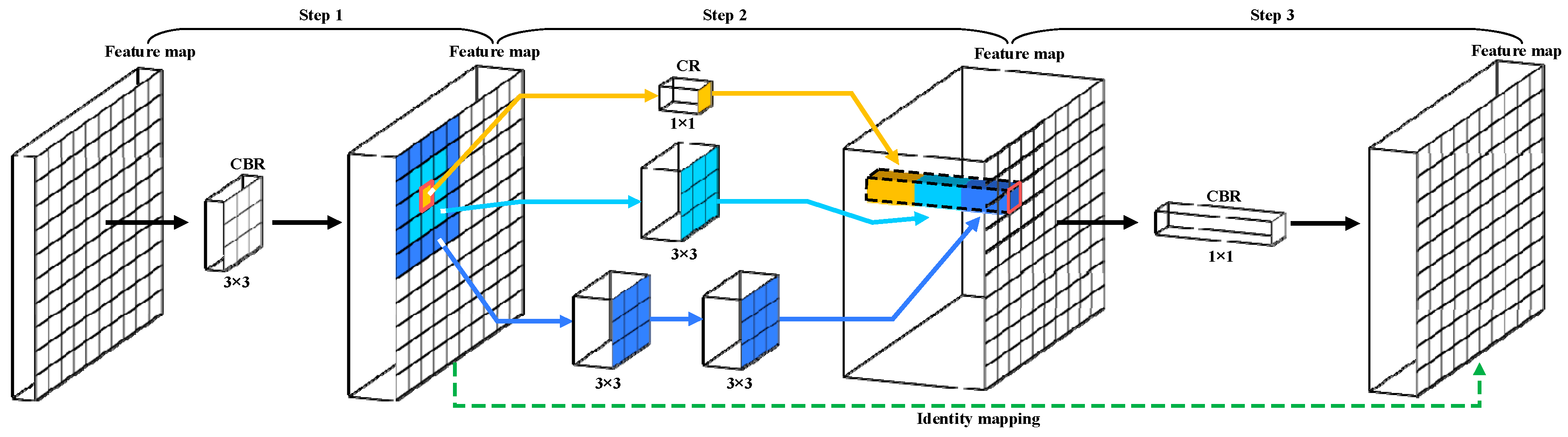
Remotesensing 13 04805 g001
Figure 2. The general structure of the MFF. The graphic does not show the specific structural changes caused by the skip connections and the dilated convolution. Meanwhile, different colors are utilized to emphasize the vital structures.
Remotesensing 13 04805 g002
Figure 3. The details of MFF_En and MFF_De. (a) The structure of MFF_En. (b) The structure of MFF_De. In the graph, N2 represents the size of the feature map, while C represents the number of the feature map channels.
Remotesensing 13 04805 g003
Figure 4. The CDSFF structural diagrams in CSD-Net. The four feature maps with different levels are coupled by CDSFF_1, CDSFF_2, CDSFF_3, and the Main Output structure in the decoding part.
Remotesensing 13 04805 g004
Figure 5. Some annotation samples from CSWV. (a,b) The original images and corresponding masks of CSWV_M21. (c,d) The original images and corresponding masks from CSWV_S6. The red regions represent clouds, the snow is represented by the blue regions, and the gray regions are the other objects.
Remotesensing 13 04805 g005
Figure 6. The proportion of cloud, snow, and background pixels in different datasets. (a) The components of L8_SPARCS. (b) The components of CSWV_M21. (c) The components of CSWV_S6.
Remotesensing 13 04805 g006
Figure 7. The loss curves over the validation subset for ablation networks. (a) The ablation comparison of MFF. (b) The ablation comparison of DS. (c) The ablation comparison of FF. (d) The ablation comparison of CL. The initial loss value is shown by the light-colored line in the figures. To better show the comparison, the original (ori.) loss curves were processed by the smoothing (smo.) function and formed more smooth dark curves. The results of the experiments showed that the MFF and CDSFF were favorable for obtaining accurate detection outcomes and for guiding the network to a stable and rapid gradient descent. However, when these modules were replaced or removed, the capacity of the network to extract the features was harmed. In a word, CSD-Net with MFF and CDSFF gained the best performance.
Remotesensing 13 04805 g007
Figure 8. Large scene visualization of cloud and snow detection results by different methods based on the L8_SPARCS dataset. The delineated areas with the green boxes were magnified to provide a more detailed visual comparison in the bottom columns.
Remotesensing 13 04805 g008
Figure 9. On the L8_SPARCS dataset, the visual comparison of cloud and snow detection results for several deep learning methods. It lists the original images, the detection results of various methods, and the ground truths one by one. The delineated areas with the green boxes were magnified to provide a more detailed visual comparison.
Remotesensing 13 04805 g009
Figure 10. Large scene visualization of cloud and snow detection results by different methods based on the CSWV_M21 dataset. The delineated areas with the green boxes were magnified to provide a more detailed visual comparison in the bottom columns.
Remotesensing 13 04805 g010
Figure 11. On the CSWV_M21 dataset, the visual comparison of cloud and snow detection results for several deep learning methods. It lists the original images, the detection results of various methods, and the ground truths one by one. The delineated areas with the green boxes were magnified to provide a more detailed visual comparison.
Remotesensing 13 04805 g011
Figure 12. Large scene visualization of cloud and snow detection results by different methods based on the CSWV_S6 dataset. The delineated areas with the green boxes were magnified to provide a more detailed visual comparison in the bottom columns.
Remotesensing 13 04805 g012
Figure 13. On the CSWV_S6 dataset, the visual comparison of cloud and snow detection results for several deep learning methods. It lists the original images, the detection results of various methods, and the ground truths one by one. The delineated areas with the green boxes were magnified to provide a more detailed visual comparison.
Remotesensing 13 04805 g013
Figure 14. The MIoU, IoUc, and IoUs of different methods. Meanwhile, the absolute difference between IoUc and IoUs was calculated and shown. (ac) The comparison of results on L8_SPARCS, CSWV_M21, CSWV_S6, respectively.
Remotesensing 13 04805 g014
Figure 15. The box graphs of accuracy metrics for various deep learning methods. (ac) The numerical distribution of MIoU, Macro-F1, and Kappa. The cross in the box represents the median of all values, while the horizontal line denotes the mean value.
Remotesensing 13 04805 g015
Figure 16. The accuracy and complexity bubble charts of different methods. (ac) The comparisons of the various methods based on the L8_SPARCS, CSWV_M21, and CSWV_S6, respectively. The various colors of circles symbolize different networks. The vertical axis is the value of MIoU, while the value of FLOPs is represented on the horizontal axis. The center of the circle corresponds to its MIoU and FLOPs, and the area of the circle reflects its parameter quantity.
Remotesensing 13 04805 g016
Figure 17. The loss curves of CSD-Net with different learning rates. (a) The complete loss curve of CSD-Net during training. (b) Partial enlargement of the loss curves in the later stages of training.
Remotesensing 13 04805 g017
Figure 18. The comparison of the three datasets based on experimental results. (a) The combination chart indicates the lowest loss over the validation subset and the highest MIoU achieved by the methods on various datasets. (b) The radar chart reflects the standard deviation of the same assessment metric for different methods.
Remotesensing 13 04805 g018
Figure 19. The accuracy curves of transfer training and direct training. In the charts, the disparities in accuracy between both training strategies were also plotted. (a) The MIoU values of both training strategies. (b) The Macro-F1 values of both training strategies.
Remotesensing 13 04805 g019
Figure 20. The examples of transfer learning prediction results on the CSWV_M21. The number at the top indicates how many epochs of transfer learning were performed on the target dataset.
Remotesensing 13 04805 g020
Figure 21. The accuracy curves of transfer training, direct training, and transfer training with dynamic learning rate. (a) The MIoU values of three training strategies. (b) The Macro-F1 values of three training strategies. Difference1 is the discrepancies in accuracy between direct training and transfer training. Difference2 represents the discrepancies in accuracy between direct training and transfer training with dynamic learning rates.
Remotesensing 13 04805 g021
Figure 22. The examples of transfer learning prediction results on the L8_SPARCS. The number at the top indicates how many epochs of transfer learning were performed on the target dataset.
Remotesensing 13 04805 g022
Figure 23. Error cases in challenging cloud and snow detection scenes. (a) The remote sensing images with detection errors. (b) The delineated areas in (a) with the green boxes were magnified to provide a more detailed visual comparison.
Remotesensing 13 04805 g023
Table 1. The detailed information of L8_SPARCS, CSWV_M21, and CSWV_S6 datasets.
NameL8_SPARCSCSWV
CSWV_M21CSWV_S6
SourceLandsat8WorldView2WorldView2
Scenes80216
ChannelsLack of band11R/G/BR/G/B
Total Pixels8 × 107~2.2 × 10⁷~2.9 × 10⁸
Pixel size30 m1–10 m0.5 m
Image size1000 × 1000 × 10Irregular size × 3Irregular size × 3
LabelFloodYesNoNo
WaterYesNoNo
ShadowYesNoNo
Shadow on wat.YesNoNo
Snow/IceYesYesYes
CloudYesYesYes
Table 2. The training details in different datasets.
DatasetTypeTrainVal.TestAllEpochsHinge Loss αDilation Rate
L8_SPARCSOriginal22060403201200.150(1,2)
Enhanced880240401160
CSWV_M21Original481620841200.120(1,2)
Enhanced1926420276
CSWV_S6Original7202181761114800.075(2,4)
Enhanced28808721763928
BiomeOriginal85981554282512,977800.200(1,2)
Enhanced34,3926216282543,433
HRC_WHUOriginal600120180900800.120(1,2)
Enhanced24004801803060
Table 3. The detection accuracy, time complexity, and spatial complexity of various ablation networks on the CSWV_S6.
Networks(a)(b)(c)(d)(e)(f)(g)(h)
Backbone
Inception V1-naive×××××××
Inception V4-A×××××××
MFF (single channel)×××××××
MFF××××
DS×××××××
DSFF×××××××
CDSFF××××
MIoU82.89%85.18%86.52%86.90%88.54%85.73%87.09%85.03%
Macro-F190.46%91.79%92.62%92.86%93.83%92.12%92.98%91.70%
Kappa86.00%89.83%90.45%90.53%91.53%90.14%90.47%89.55%
OA94.09%95.87%96.13%96.14%96.56%95.99%96.11%95.73%
Macro-Pc88.56%90.37%91.70%91.39%92.84%90.99%91.82%90.55%
Macro-Rc93.15%93.40%93.60%94.46%94.91%93.33%94.29%93.02%
GFLOPs 140.2687.8887.9288.0688.0662.1680.356.44
Parameters (M) 23.627.467.617.617.615.518.856.09
1 1 M = 1 × 10⁶; 2 1 GFLOPs = 1 × 10⁹ FLOPs.
Table 4. The cloud and snow detection accuracy comparisons on the various datasets.
DatasetMethodMIoUMacro-F1KappaOAMacro-PcMacro-Rc
(a) L8_SPARCSU-Net79.94%88.47%85.07%94.60%90.43%86.80%
PSPNet79.17%88.02%82.12%93.45%89.76%86.68%
DeeplabV3+66.26%78.74%70.87%87.93%75.50%83.77%
RSNet79.60%88.17%85.94%94.79%90.98%86.87%
SegNet-M75.81%85.56%81.57%93.52%88.99%82.70%
MSCFF83.59%90.83%87.77%95.51%92.65%89.55%
GeoInfoNet75.77%85.72%79.93%92.09%86.39%87.15%
CDnetV283.19%90.59%86.02%94.77%89.69%91.53%
CSD-Net87.24%93.08%89.47%96.02%91.85%94.40%
(b) CSWV_M21U-Net82.41%90.18%86.77%92.85%91.61%89.04%
PSPNet75.59%85.78%79.95%89.04%86.26%85.45%
DeeplabV3+69.51%81.44%74.78%85.53%79.68%84.58%
RSNet85.06%91.82%88.37%93.68%92.82%91.08%
SegNet-M81.10%89.38%85.19%91.94%90.03%88.81%
MSCFF85.91%92.33%89.27%94.12%92.13%92.58%
GeoInfoNet79.68%88.52%83.40%90.75%88.50%89.06%
CDnetV283.65%91.01%87.02%92.86%90.54%91.51%
CSD-Net87.05%93.01%90.01%94.51%92.85%93.19%
(c) CSWV_S6U-Net86.48%92.61%90.00%95.89%90.62%94.89%
PSPNet86.62%92.71%89.99%95.92%91.79%93.79%
DeeplabV3+81.43%89.51%85.74%94.11%87.29%92.10%
RSNet84.53%91.43%88.44%95.26%91.25%92.23%
SegNet-M83.30%90.96%88.91%95.50%89.22%92.58%
MSCFF86.63%92.69%90.51%96.14%91.93%93.60%
GeoInfoNet85.45%92.00%88.95%95.46%90.32%93.88%
CDnetV286.53%92.63%90.59%96.20%91.88%93.42%
CSD-Net88.54%93.83%91.53%96.56%92.84%94.91%
Table 5. The value of floating point operations, the number of parameters, and the time cost for several methods.
Test ImageModelFLOPs (GFLOPs) 1Parameters (M) 2Time Cost (s)
CSWV_S6 test subset
Image size:512 2
Image number: 176
U-Net219.5934.515.3797 ± 0.1269
PSPNet184.546.714.6257 ± 0.3248
DeepLabV3+102.9441.053.0638 ± 0.0591
RS-Net56.037.852.8704 ± 0.3622
SegNet-M201.734.925.0814 ± 0.3821
MSCFF354.7951.889.2112 ± 0.1795
GeoInfoNet99.8314.666.6706 ± 0.5881
CDnetV270.1367.094.022 + 0.7158
CSD-Net88.067.614.4721 ± 0.1397
1 1 M = 1 × 10⁶; 2 1 GFLOPs = 1 × 10⁹ FLOPs.
Table 6. Comparison of CSD-Net accuracy with different dilation rates.
Dilation RateCSWV_S6CSWV_M21L8_SPARCS
MIoUMacro-F1MIoUMacro-F1MIoUMacro-F1
No dilation85.0491.7786.6792.8086.4392.60
(1, 2)86.3492.5387.0593.0187.2893.10
(2, 2)87.3393.1085.7092.2187.2893.09
(2, 3)86.1192.3684.1491.2781.9889.81
(2, 4)88.5493.8384.7191.6285.4291.97
(3, 3)86.1692.4283.5890.9385.7992.20
Table 7. Comparison of CSD-Net accuracy with different dilation rates.
Hinge Loss αCSWV_S6Hinge Loss αCSWV_M21Hinge Loss αL8_SPARCS
MIoUMacro-F1MIoUMacro-F1MIoUMacro-F1
α = 086.9092.86α = 084.4891.49α = 085.0891.78
α = 0.0684.3191.31α = 0.1086.1792.50α = 0.1287.0593.01
α = 0.0788.2993.68α = 0.1184.7891.67α = 0.1386.7092.75
α = 0.07588.5493.83α = 0.1287.0593.01α = 0.1485.2691.89
α = 0.0888.0093.51α = 0.1385.7792.26α = 0.1587.2893.10
α = 0.0987.0492.94α = 0.1486.0592.42α = 0.1686.8193.01
Table 8. Quantitative evaluation results of CSD-Net with different learning rates.
Learning RateMIoUMacro-F1KappaOAMacro-PcMacro-Rc
0.0000176.53%86.14%82.98%92.91%86.13%87.47%
0.0000582.81%90.37%87.17%94.69%88.92%92.18%
0.000188.54%93.83%91.53%96.56%92.84%94.91%
0.000583.85%91.04%87.42%94.75%88.34%94.25%
0.00187.95%93.48%91.21%96.44%92.31%94.76%
0.00585.85%92.25%89.16%95.53%90.36%94.36%
0.0182.58%90.28%85.88%93.99%86.96%94.42%
0.0583.46%90.70%88.49%95.29%89.43%92.10%
Table 9. The quantitative evaluation comparison on the HRC_WHU dataset.
MethodIoUF1-ScoreKappaOA
U-Net86.23%92.60%87.78%94.16%
PSPNet84.27%91.46%86.21%93.49%
DeepLabV3+82.57%90.45%84.14%82.40%
RS-Net88.37%93.83%89.72%95.07%
SegNet-M85.77%92.34%87.28%93.91%
MSCFF85.89%92.41%87.54%94.07%
GeoInfoNet83.02%90.72%84.43%92.50%
CDnetV285.81%92.36%87.10%93.76%
CSD-Net89.65%94.54%90.97%95.68%
Table 10. The quantitative evaluation comparison on the Biome dataset.
MethodIoUF1-ScoreKappaOA
U-Net70.88%82.96%75.43%89.51%
PSPNet74.22%85.20%78.48%90.73%
DeepLabV3+70.12%82.43%74.56%89.09%
RS-Net73.88%84.98%78.28%90.70%
SegNet-M74.74%85.54%78.73%90.73%
MSCFF74.89%85.64%78.95%90.86%
GeoInfoNet70.93%82.99%75.12%89.23%
CDnetV275.61%86.11%79.74%91.25%
CSD-Net76.89%86.99%80.71%91.53%
Publisher’s Note: MDPI stays neutral with regard to jurisdictional claims in published maps and institutional affiliations.

