Efficient and Safe Robotic Autonomous Environment Exploration Using Integrated Frontier Detection and Multiple Path Evaluation

Abstract

Autonomous exploration and remote sensing using robots have gained increasing attention in recent years and aims to maximize information collection regarding the external world without human intervention. However, incomplete frontier detection, an inability to eliminate inefficient frontiers, and incomplete evaluation limit further improvements in autonomous exploration efficiency. This article provides a systematic solution for ground mobile robot exploration with high efficiency. Firstly, an integrated frontier detection and maintenance method is proposed, which incrementally discovers potential frontiers and achieves incremental maintenance of the safe and informative frontiers by updating the distance map locally. Secondly, we propose a novel multiple paths planning method to generate multiple paths from the robot position to the unexplored frontiers. Then, we use the proposed utility function to select the optimal path and improve its smoothness using an iterative optimization strategy. Ultimately, the model predictive control (MPC) method is applied to track the smooth path. Simulation experiments on typical environments demonstrate that compared with the benchmark methods, the proposed method reduce the path length by 27.07% and the exploration time by 27.09% on average. The real-world experimental results also reveal that our proposed method can achieve complete mapping with fewer repetitive paths.

1. Introduction

Autonomous exploration enables robots to be capable of actively perceiving the environment, which has played an increasingly important role in various applications, such as monitoring environmental quality [1,2], precision agriculture [3], search and rescue [4,5,6], and open-sea exploration [7,8]. There has been some valuable work on navigation using GNSS [9,10], but in most cases, indoor robots can only rely on their carried sensors for navigation. However, the limited perception range of the sensor and the absence of any prior information about the surrounding environment pose a significant challenge for the robot to make optimal decisions. In addition, the restricted battery capacity of robots makes efficient environmental exploration essential.

Many researchers have proposed various autonomous exploration methods in recent years, which can be divided into frontier-based methods [11,12,13,14], information-based methods [15,16], and hybrid methods [17]. Different types of maps are applied to autonomous exploration, such as methods [11,18,19,20] based on occupancy grid map, methods [21,22] based on topological maps, and methods [23] based on feature maps. The frontier-based method is intuitive and efficient, and an occupancy grid map can be used for efficient path planning. We propose a frontier-based exploration method based on an occupancy grid map. The frontier-based exploration method advocates the constant acquiring of frontiers, an evaluation of the frontiers, and a move towards the most promising frontier in each exploration step. The following problems at each stage persist.

Frontier detection is the cornerstone of autonomous exploration. Failure to obtain the frontier in time will cause the robot to explore an area back and forth. Traditional methods [13] deal with the entire map to obtain the frontier, but the efficiency decreases as the map increases. Furthermore, most of the existing methods still consider a single source to obtain frontiers. How to effectively maintain the frontiers in the exploration process and eliminate inefficient frontiers in time is also an urgent problem to be solved and has largely been ignored in the literature. An integrated frontier detection and maintenance method is proposed in this work. We obtain two types of frontiers by detecting changes in the active area on the occupancy grid map and lidar data. We propose the use of the Euclidean distance map to perform incremental maintenance on the frontier.

The evaluation of the frontier determines the next promising target. Some exploration methods [11,24,25] directly use Euclidean distance instead of the actual path length, which will affect the decision making in complex scenarios. Some methods require multiple path generations, resulting in a waste of computing resources. Incomplete evaluation metrics cannot accurately evaluate unexplored frontiers effectively [13,15]. We propose a novel utility function to carry out a reasonable assessment of frontiers, which considers information gain, path cost, consistency of robot movement, and valid lidar data acquisition.

For path planning, using local paths to explore the environment often requires other strategies to solve the local minimum problem. The rapidly exploring random trees (RRT) path planning method [26] has a tortuous path. Some search planning algorithms [11,25] focus on the generation of the shortest path and ignore the clearance and smoothness of the path. We propose a multiple paths generation method based on fast marching [27]. An iterative path optimization strategy is put forward to improve the smoothness of the selected path.

Our main contributions include the following aspects.

• We propose an integrated frontier detection and maintenance method. A complete environmental exploration can be achieved by sufficient frontier detection and incrementally maintaining reachable and informative frontiers.
• A multiple path generation method is proposed using the wavefront propagation trend of the fast-marching method and a well-designed velocity field to generate safe paths with a good view.
• A multi-object utility function is proposed for frontier evaluation to obtain the optimal path, improving exploration efficiency. A path smoothing method with dynamic parameter adjustment improves the smoothness of the optimal path.

We propose a complete framework for autonomous robot exploration in unknown environments and verify the effectiveness and practicability of the proposed framework through sufficient experiments.

The remaining article is organized as follows. In Section 2, we introduce related work in autonomous exploration. In Section 3, we provide the problem statement. Our proposed method is presented in Section 4. In Section 5, we provide the experiments and results both in simulated and real-world environments. In Section 6, we provide the discussion of this work. Lastly, in Section 7, we provide the conclusion of this work and provide future directions.

2. Related Works

2.1. Frontier Detection Methods

Yamauchi et al. [13] proposed the concept of frontier-based exploration; however, frontier detection requires the processing of the entire map each time—as the map increases, the frontier detection efficiency gradually decreases. Some researchers have worked on the efficient detection of the frontier. Umari et al. [11] innovatively proposed using global and local rapidly exploring random trees [26] to detect frontiers in 2D and 3D scenes. Keidar et al. [12] proposed efficient frontier detection methods, such as the wavefront frontier detector (WFD) and the fast frontier detector (FFD) but did not consider whether the frontier was reachable. Unreachable frontiers will produce invalid paths, waste computing resources, and make exploration inefficient. The work in [19] further considered the extraction of reachable frontiers and only incrementally processed the modified portions of the occupancy to obtain safe and valid frontiers. The safe and reachable frontier detection generator (SRFDG) [27] uses laser data to efficiently obtain two types of fronters and maintains a global topological map. However, due to the uncertainty of the pose during the mapping process, the frontier cannot always be effectively obtained based on laser data alone. At the same time, this method ignores the timely detection of the changes on the map. Different from the above method, which detects frontiers from a single source, our method uses an occupancy grid map and lidar data to obtain frontiers together. The proposed method only deals with a fixed size active area, which reduces the computational burden. Meanwhile, we propose a method of deleting inefficient frontiers.

2.2. Decision-Making Methods

Some methods only consider a single evaluation metric. Yamauchi et al. [13] only considered the distance between the frontier and the robot as the evaluation metric, ignoring the different information acquisition between frontiers. Stachniss et al. [20] proposed an evaluation strategy to evaluate each action that trades off the expected information gain cost and reduces localization uncertainty. To prevent the robot becoming trapped in the cubicle areas, Gao et al. [28] added the consideration of the rotation angle to the evaluation function, allowing the robot to explore as far as possible along the current direction. However, this method increases the complexity of adjusting the parameters. Unlike the above methods, we propose a method that considers multiple metrics for evaluating frontiers with only two adjustable parameters, which uses the distance map to efficiently evaluate the impact of different paths on the mapping.

2.3. Path-Planning Methods

Fang et al. [29] proposed an improved dynamic window approach [30] with a new trajectory evaluation function to achieve local exploration. Lauri et al. [31] modeled the robot’s autonomous exploration as a partially observable Markov decision process (POMDP) and obtained the most informative local trajectory through forward simulation algorithms with an open-loop approximation. Ding et al. [32] proposed to obtain multiple local trajectories and used information entropy to evaluate multiple trajectories. However, the above methods may have had local minimum problems in some complicated scenarios. Therefore, some of the methods solve the local minimum problem by integrating the frontier-based exploration method [31] or re-planning the global path [32]. Bircher et al. [33] used the RRT method to explore and generate a path. However, the randomness of the RRT tree has poor smoothness and hinders the robot’s rapid movement. Some advanced improvement methods such as RRT* [34], qRRT [35], and RRdT* [36] improve the path quality of RRT. A class of common methods [11,24,25] uses the A* algorithm for path planning, sometimes resulting in paths close to obstacles. The fast-marching method [37] is local minimum free and complete and has been widely used in path planning [38,39,40]. The method in [41] performs the fast-marching method to obtain a path on the gradually acquired environment map transformed using the logarithm of the extended Voronoi. However, this work ignored ensuring that the ranging sensor collected valid data when generating the path. When the robot executes such a path, it may affect the quality of positioning. We use the Euclidean distance map to generate a reasonable velocity field to avoid the above problem and generate multiple paths for evaluation. Usenko et al. [42] proposed a trajectory optimization method using the uniform B-spline. Zhou et al. [43] further improved the optimization efficiency. Inspired by the above methods, to facilitate the tracking of non-holonomic constrained robots, we propose a path optimization method with dynamic parameter adjustment to improve the smoothness of the path.

According to the characteristics of our proposed work, we give a comparison with related works in

Table 1. Comparison of our proposed work with related works.

References	Map Type			Frontiers Detection			Decision Making			Path Planning			Experimental Scenario
	Occupancy Grid Map	Topological Map	Feature Map	Occupancy Grid Map	Lidar Data	Lidar Detection Range	Lidar Data Quality	Actual Path	Movement Consistency	Multiple Path Generation	Path Smoothing	Path Clearance	Simulation	Real-World
[11]	√	–	–	√	–	–	–	–	–	–	–	–	√	√
[12]	√	–	–	√	√	√	–	–	–	–	–	–	√	–
[13]	√	–	–	√	–	–	–	–	–	–	–	–	√	√
[15]	√	–	–	√	–	–	–	–	–	–	–	–	√	√
[17]	√	√	–	√	–	√	–	√	–	√	√	–	√	√
[18]	√	–	–	√	–	–	–	–	–	–	–	–	√	√
[19]	√	–	–	√	–	√	–	–	–	–	–	–	√	–
[20]	√	–	–	√	–	–	–	√	–	√	–	–	√	√
[21]	√	√	–	√	–	–	–	√	–	–	–	–	√	√
[23]	–	–	√	–	–	–	–	√	–	√	–	–	√	√
[24]	√	–	–	√	–	–	–	–	–	–	–	–	√	√
[25]	√	–	–	√	–	–	–	–	–	–	–	–	√	√
[37]	√	√	–	–	√	–	–	√	–	–	–	–	√	√
[28]	√	–	–	√	–	–	–	–	√	–	–	–	√	√
[29]	√	–	–	√	–	–	–	–	–	√	–	–	√	√
[41]	√	–	–	√	–	–	–	–	–	–	–	√	√	–
Our work	√	–	–	√	√	√	√	√	√	√	√	√	√	√

.

3. Problem Statement

We first list the common symbols and meanings used in

Table 2. Common symbols and meanings used in this article.

$ℳ$	Occupancy grid map.
$f$	Single frontier.
$F_w$	The frontier warehouse is used to store the frontiers obtained in each exploration cycle.
$F_o$	Stores the frontiers obtained from the active area of occupancy grid map $ℳ$.
$F_l$	Stores frontiers acquired using lidar data.
$F$	The clustered frontiers.
$F_s$	Frontiers with valid paths.
${\theta }_{Max}$	The maximum angular deviation that can be followed.
$k_P$, $k_{\phi }$, $k_I$	The coefficient in utility function, where $k_{\phi }$ is only related to the physical characteristics of the robot.
$D_l$	Lidar max range.
$\mu$	The confidence range ratio.
$T$, $\tau$	$T$ represents the path which is composed of waypoint $\tau$.
$d(·)$	Distance function, obtain the distance between any position on the map and the obstacle.

, then give the problem statement.

Define $\mathcal{S}\subset {ℝ}^2$ as the environment to be explored. We used the occupancy grid map $ℳ$ to model the 2D environment $\mathcal{S}$. $ℳ$ consists of many grids $s_i$, $i\in [1,N]$ and $N$ is the number of grids. The value of $s_i$, $i\in [1,N]$ indicates the probability of being occupied. Before the exploration, all the grids are marked as ${\mathcal{S}}_{unknown}$. During continuous exploration, an increasing number of grids marked ${\mathcal{S}}_{known}$ begin to appear, and ${\mathcal{S}}_{known}$ is divided into occupied grids and free grids, ${\mathcal{S}}_{known}=\{{\mathcal{S}}_{occupied},{\mathcal{S}}_{free}\}$. In this article, the discrete grids located in the frontier area are referred to as frontiers.

Problem: Given occupancy grid map $ℳ$ find the next most promising frontier $f$ with the optimal path $T^{*}$ which is followed by the robot.

The problem is solved repetitively at every exploration cycle. Use $ℳ$ to detect the unexplored frontiers and calculate the corresponding paths to those frontiers. Find the next promising fronter $f$ using the utility function. The robot moves along the optimal path $T^{*}$ attached to $f$, and updates $ℳ$ with the up-to-date sensor reading online, such as 2D lidar, constantly changing ${\mathcal{S}}_{unknown}$ to ${\mathcal{S}}_{known}$. The newly generated $ℳ$ is used for the next exploration cycle until the map of the entire environment is completed.

4. Proposed Method

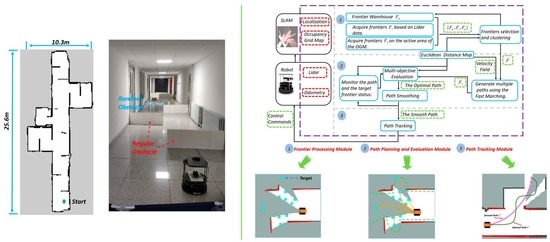
4.1. Method Overview

The autonomous exploration framework consists of the frontier processing module, the path planning and evaluation module, and the path tracking module, as shown in Figure 1. The robot provides lidar and odometry data and responds to control commands. The SLAM module simultaneously generates the occupancy grid map $ℳ$ and localizes the robot. The blue rectangles represent the crucial functions. The green dashed rectangles represent the information to be transmitted. The black rectangles represent the external inputs of the system.

Algorithm 1 shows the process of autonomous exploration. Each module can interact with external inputs, such as lidar data, localization, and occupancy grid map $ℳ$. The execution of the exploration cycle is awakened through a timing trigger and a re-planning trigger (line 1). The timing trigger mechanism can adapt to environmental changes. The re-planning trigger mechanism continuously detects the safety of the path and the information acquisition of the target to reduce unnecessary forward distance and ensure that the path is collision-free. The Bayesian filter and log-odds ratio formulation are used to update the grid map. The Euclidean distance map can obtain the distance between any position and the obstacle on the map, which can be used for autonomous robot exploration. The updated $ℳ$ and a dynamic variant of the brushfire algorithm [44] are used to obtain the Euclidean distance map, where the unknown and free areas are regarded as free (line 2). The frontier detection and maintenance method incremental acquires and maintains frontiers for the subsequent modules (line 3). Then, multiple paths planning and evaluation generates the OptimalPath by evaluating multiple paths (line 7). The OptimalPath is further processed to improve its smoothness (line 8). Finally, the path is tracked by the robot, and the data observed by the robot are also updated (line 9). When there is no effective frontier, the exploration is complete (lines 4–6).

Algorithm 1. Autonomous Exploration.
Input: $ℳ$, RobotLocation, LidarData,$F_w$←∅, ExplorationFlag←True
Output: Complete map of environment
1	whileExplorationFlag=True∧(ReplanTrigger=True∨ TimingTrigger=True) do
2	DistanceMap←UpdatingEuclideanDistanceMap($ℳ$);
3	$F$←Frontier Detection and Maintenance($F_w$,$ℳ$,
	DistanceMap, RobotLocation, LidarData);
4	if $F$ = ∅ then
5	ExplorationFlag = False;
6	break;
7	end
8	OptimalPath←Multiple paths planning and  evaluation($F$,$ℳ$, DistanceMap, RobotLocation);
9	SmoothPath←Smooth the path$({\phi }_1$,${\phi }_2$, DistanceMap, OptimalPath);
10	Publish Smooth Path to Path Tracking Module;
11	end

4.2. Frontier Detection and Maintenance

As shown in Algorithm 2, this method inputs updated $ℳ$, robot localization, lidar data, and outputs frontiers set $F$ for path planning and evaluation. $F_o$ stores the frontiers obtained from the active area of $ℳ$ and $F_l$ stores frontiers acquired using lidar data. The frontier warehouse $F_w$ incrementally stores the frontiers obtained during the exploration process and records all the acquired but unexplored areas. Using the lidar detection range, $ℳ$, and robot location, we can obtain the frontier $F_o$ by searching the active area (lines 2,3).

Algorithm 2. Frontier Detection and Maintenance.
Input: $ℳ$, RobotLocation, LidarData, $F_w$, DistanceMap
Output: $F$
1	$F_o$←∅, $F_l$←∅;
2	ActiveArea← AquireActiveArea ($ℳ$, RobotLocation, LidarData);
3	$F_o$← SearchFronteirsOnOGM (ActiveArea);
4	SetObstacle (RobotLocation, DistanceMap);
5	foreach frontier f in {$F_o$,$F_w$} do
6	if GetDistance(f)<safe dist ∨ (GetNearestObsCood (f)=
	RobotLocation∧|| f- RobotLocation || <$D_l$) ∨GetInformationCost<
	InfoThreshhold then
7	remove f;
8	end
9	end
10	$F_l$← AquireFrontiersUsingLidarDate (LidarData, RobotLocation);
11	foreach frontier f in$F_l$do
12	if GetInformationCost<InfoThreshhold then
13	remove f;
14	end
15	end
16	RemoveObstacle(RobotLocation, DistanceMap);
17	if {$F_o$,$F_l$,$F_w$}= ∅ then
18	$F$←∅;
19	return;
20	else
21	$F$← Cluttering($F_o$,$F_l$,$F_w$);
22	$F_w$←∅, $F_w$←$F$;
23	end

However, some frontiers are too close to the robot, as shown by the red dots in Figure 2b. If these frontiers are selected as targets, the efficiency of robot exploration will decrease. The method of connecting the robot to all frontiers within the scanning range of lidar and performing collision detection is computationally intensive and may remove frontiers that facilitate positioning. The distance map can be updated efficiently by only updating affected parts without updating the entire map. Based on the above considerations, we take advantage of the local update feature of the dynamic distance map to remove inefficient frontiers. The local distance map can be changed by setting the robot as a virtual obstacle, as shown in Figure 2c. The inefficient frontiers within the lidar range can be eliminated by querying whether the nearest obstacle of those frontiers is the robot’s position. In addition, the current $F_o$ and $F_w$ obtained in the previous cycle are processed to remove inefficient and unreachable frontiers (lines 4–7). To improve the efficiency, we use the ray-casting method to simulate lidar to sample the environment and use the Breshmen method [45] to obtain the corresponding grids. When the number of unknown grids around a frontier is less than the threshold, it is considered that there is too little information.

The lidar data of undetected obstacles are processed to obtain potentially accessible frontiers to accelerate the autonomous exploration of the environment, as shown in Figure 3. The green dotted curve in Figure 3a shows the potential unexplored area $\stackrel{⌢}{AB}$ which presents the end of the continuous and collision-free laser beam. First, whether the midline of the acquired area $\stackrel{⌢}{AB}$ can make the robot collision-free is determined. If the above condition is satisfied, further analysis of the area $\stackrel{⌢}{AB}$ can be performed.

$$\begin{array}{l}{\alpha }_1=(n+1)\cdot {\alpha }_0-2d_1/(D_l-d_0)\\ {\alpha }_2=2r/(D_l-d_0)\\ m=\lfloor {\alpha }_1/{\alpha }_2\rfloor \end{array}$$

(1)

We can further extract the safe and feasible area $\stackrel{⌢}{A^{\prime }{B}^{\prime }}$, as shown in the green line. The red circle indicates the robot’s footprint, and $d_0$ is slightly larger than the robot radius $r$, and $d_1=2d_0$. The ${\alpha }_0$ is the angular resolution of the lidar. The $n$ is the continuous and non-collision laser beam, and the $D_l$ is the maximum detection range of lidar. Using Equation (1) to process the acquired area $\stackrel{⌢}{AB}$, we can obtain $m$ uniformly distributed frontiers. Then, we can calculate the position of these frontiers in the lidar coordinate system and transform these frontiers into the map coordinate system. Finally, we can keep the information-rich frontiers in $F_l$ (lines 8–11).

After the above processing, if there are unexplored frontiers, we can use the mean-shift clustering method [46] to remove redundant frontiers as it has only one parameter (bandwidth) and the parameter has a clear physical meaning (line 17). However, using the mean-shift method may cause the frontier to be unreachable or contain less information after clustering. The frontier with the smallest Euclidean distance from the cluster center in a cluster of frontiers is selected as the output to solve this problem. This method preserves the clustering characteristics as much as possible and ensures that the points after the clustering are informative and collision-free. The frontier set $F$ is used for subsequent path planning and evaluation, and $F_w$ is updated to achieve complete mapping (line 18).

4.3. Multiple Paths Planning and Evaluation

The process of multiple paths planning and evaluation is divided into three parts. We use the fast-marching method with a well-designed velocity field to generate multiple paths from the robot position to the unexplored frontiers. Then, we evaluate those paths to obtain the optimal path, which corresponds to the most promising frontier using the proposed utility function. Finally, the smoothness of the path is further improved.

4.3.1. Multiple Path Generation Using Fast Marching

Fast marching is a numerical method for simulating the spread of a wavefront which can be represented by the Eikonal differential equation [27]:

$$|\nabla T(x)|=\frac{1}{f(x)}$$

(2)

The left side of the equation depicts the function of the arrival time and $f(x)$ represents the velocity of different positions $x$. The velocity function $f(x)$ determines the propagation velocity at different positions and is the key to the fast-marching method. When $f>0$, the wavefront always spreads outward, and the wavefront will only pass through each grid on the map once. We used the two characteristics of the fast-marching method for multiple paths planning.

Characteristic 1: Design an appropriate velocity field to generate a path with good clearance.

$$f(x)=\{\begin{array}{cc}d(x)\hfill & (0<d(x)<D_l)\hfill \\ 0\hfill & (d(x)\ge D_l)\hfill \\ 0\hfill & (d(x)\le r)\hfill \end{array}$$

(3)

The distance map can be transformed into a velocity field using Equation (3). The $d(x)$ is the distance corresponding to position $x$, and the $D_l$ is the maximum detection range of lidar. If the $d(x)$ of a location $x$ on the map is greater than $D_l$ or less than the robot radius r, the speed is set to 0. The velocity function ensures the wavefront will not extend to these locations during the path generation process. By simulating a wave expanded from the start point, we can obtain the arrival time of each point on the map. The closer a certain position $x$ to an obstacle, the lower the corresponding wavefront spread speed of the position will be generated, which leads to a later arrival time at the position. We can trace the path from the target point to the starting point along the descending direction of the arrival time gradient and obtain the path with the minimal arrival time. The path is also away from obstacles and ensures that lidar can extract the environmental features to facilitate positioning.

Characteristic 2: The wavefront propagates from near to far to generate multiple paths. The robot is used as the starting point when performing fast marching. When the far frontier is selected as the target, the frontiers near the robot will often be covered as the wavefront expands. Coincidentally, from the perspective of exploration, the robot usually explores from near to far to avoid repeatedly visiting a certain area. Nevertheless, as the map becomes larger, more computing resources will be consumed. Moreover, too many paths to be evaluated also put pressure on the evaluation module. To reduce the computational burden, we formulate the following rules.

1. Select $t$ frontiers closest to the robot in the set $F$ as the set $F_d$, $F_d=\{f_1,f_2,\cdot \cdot \cdot ,f_t\}$ and $F_d\subseteq F$.

2. Set the frontier $f_i\in F_d$, $i\in [1,t]$ which is the farthest from the robot, as the target point.

3. If multiple frontiers satisfy rule 2, select the closest one to the obstacle as the target point. Finally, frontiers with valid paths are stored in set $F_s$, $F_s\subseteq F_d$.

Figure 4 shows the process of generating multiple paths. The fast-marching method is executed using the generated velocity field and the target point selected using the above rules. The fast-marching method only expands once to obtain multiple paths, with the time complexity of $O(Nlog(N))$ and $N$ is the number of free discretization grids on the map. In Figure 4, multiple paths connecting with unexplored frontiers are represented by yellow curves.

Theorem 1.

Each frontier $f$, $f\in F_s$ has a valid path.

Proof of Theorem 1.

After clustering, all frontiers are located in different grids of map, and there are no overlapping frontiers. The fast-marching method has been proven to be complete [47]. Considering all frontiers in $F_d$, when a frontier is within the extended range of the wave, the path from the frontier to the starting point can be found. Otherwise, there is no path with a frontier that is out of range of the wave. The frontier $f$, $f\in F_d$ with a valid path is stored in set $F_s$, ensuring each $f$, $f\in F_s$ has a valid path. □

4.3.2. Path Evaluation

After path planning, we can obtain the set $F_s$, $F_s=\{f_1,f_2,\cdot \cdot \cdot ,f_n\}$ and each $f_i$, $i\in [1,n]$, has an attached path $T$. Path $T$ is composed of waypoints ${\tau }_j$, $j\in [1,m]$, where $m$ is the number of waypoints. We put forward a utility function to find the most promising frontier $f_i$, $f_i\in F_s$ and $i\in [1,n]$, and the attached path is regarded as the optimal path and represented by $T^{*}$. The utility function considers information gain, path cost, consistency of robot movement, and valid lidar data acquisition. Therefore, each candidate frontier $f_i\left\{L_i,I_i,P_i\right\}$, $i\in [1,n]$ has three attributes: $L$ represents lidar data acquisition cost, $I$ represents the information gain, and $P$ represents the path cost.

1. Lidar data acquisition cost $L$

For $f_i$, $f_i\in F_s$ and $i\in [1,n]$, we use Equation (4) combined with the distance function $d(\cdot )$ to evaluate the lidar data acquisition quality of the attached path $T$.

$$l({\tau }_j)=\{\begin{array}{cc}1\hfill & (d({\tau }_j)<\mu \cdot D_l)\hfill \\ -(d({\tau }_j)-\mu \cdot D_l{)}^3+1\hfill & (d({\tau }_j)\ge \mu \cdot D_l)\hfill \end{array}$$

(4)

$$L(f_i)={\displaystyle \sum _{j=1}^{m}l({\tau }_j)}/m$$

(5)

When the distance between the waypoint ${\tau }_j$, $j\in [1,m]$ and the obstacle is less than $\mu \cdot D_l$, assign a constant value; otherwise, the value will decrease rapidly as the distance increases. $\mu$ is set by the user representing the confidence range ratio of the lidar. Take the average of the values of all waypoints to obtain the lidar data acquisition cost $L$.

2. Information gain $I$

The entropy $H$ is an effective tool to describe the uncertainty of the map [20]. The process of exploration is a process of continuously reducing map uncertainty $H$.

$$H(S)=-{\displaystyle \sum _{i=1}^{N}p(s_i)}\log (p(s_i))$$

(6)

Mutual information $I$ is used to represent the reduced uncertainty after the robot executes a certain path $T$ where $p(s_i)$ represents the occupancy probability of grid $s_i$, $i\in [1,N]$ and $N$ is the number of grids.

$$I\left(\mathcal{S};T\right)=H(\mathcal{S})-H\left(\mathcal{S}\mid T\right)$$

(7)

To improve computational efficiency, the information gain $I$ is only processed at the target point. Furthermore, the ray-casting and Breshmen methods are used to obtain the corresponding grid and calculate the corresponding information gain.

3. Path cost $P$

We can calculate the path length cost $P$ from path $T$. In addition, in order to maintain the consistency of the motion and avoid back-and-forth maneuver, we calculate the angle $\theta$ between the initial part of the path and the orientation $\phi$ of the robot.

$$\theta ={\cos }^{-1}\frac{({\tau }_2-{\tau }_1)·\phi }{\Vert {\tau }_2-{\tau }_1\Vert ·\Vert \phi \Vert }$$

(8)

This item has less influence on the exploration process than other items. We design the measurement of the consistency of the motion as a coefficient multiplied by the path cost $P$. This avoids adding new items to the utility function. When the initial path and the robot direction vector are greater than ${\theta }_{Max}$, we set the coefficient $k_{\phi }$ to 1; otherwise, it is set to the user set value (less than 1). This can ensure that even a slightly longer path with an appropriate angle can be selected to ensure the continuity of movement and improve the efficiency of exploration. The value of ${\theta }_{Max}$ considers the actual tracking condition of the robot. Equation (8) gives the complete utility function.

$$U\left(f_i\left\{I_i,P_i,L_i\right\}\right)=\frac{k_I{I}_i}{\overline{I}}-\frac{k_{\phi }{k}_P{P}_i}{\overline{P}}+L_i,\hspace{1em}i\in [1,n]$$

(9a)

$$\overline{I}={\displaystyle \sum _{i=1}^n{I}_i/n}$$

(9b)

$$\overline{P}={\displaystyle \sum _{i=1}^n{P}_i/n}$$

(9c)

The coefficient $k_{\phi }$ is only related to the physical characteristics of the robot. We need only adjust the coefficients $k_I$ and $k_P$ to realize efficient exploration of different environments. The information gain $I$ and the path cost $P$ are normalized to remove their unit.

$$\underset{f_i\in F_s}{\arg \max }U\left(f_i\left\{I_i,P_i,L_i\right\}\right)$$

(10)

Each time the robot chooses the frontier $f_i\in F_s$, $i\in [1,n]$, with maximum $U$ as the target region to be explored. The selected target region is more informative and near the robot. At the same time, the attached $T^{*}$ of $f_i$ can promote the consistency of robot movement and confirm the lidar obtain effective data.

4.3.3. Path Smoothing and Tracking

The path $T^{*}$ generated by the fast-marching method is affected by the environment, and the smoothness of the path needs to be improved. An optimization method of dynamically adjusting parameters is applied to smooth the path to facilitate the further tracking of the robot.

Considering that the B-spline has some characteristics, such as the fact that its derivative is still B-spline, and control points are located inside the convex hull, we use B-spline to represent the path and further optimize its control points. The $N+1$ control points $\{P_0,P_1,\cdots ,P_N\}$, $P_i\in {ℝ}^2$, can define a $\lambda \mathrm{th}$ B-spline and knot vector $[t_0,t_1,\cdots ,t_M]$, $t_m\in R$, where $M=N+\lambda +1$. A B-spline is parameterized by $t$, $t\in [t_{\lambda },t_{M-\lambda }]$, and a uniform B-spline with each knot span has identical value $\Delta t$. We can obtain the position at the corresponding parameter $t$ using Equation (10) and $t$ is normalized as $\alpha (t)=(t-t_m)/\Delta t$, where $t\in [t_m,t_{m+1}]\subset [t_{\lambda },t_{M-\lambda }]$. $M_{p+1}$ is the constant matrix determined by $\lambda$ [48].

$$\begin{array}{c}T(\alpha (t))=\alpha {(t)}^T{M}_{\mathrm{p}+1}P\hfill \\ \alpha (t)={[{\alpha }^{\lambda }(t),{\alpha }^{\lambda -1}(t),\cdots ,\alpha (t),1]}^T\hfill \\ P={[P_{i-\lambda },P_{i-\lambda +1},P_{i-\lambda +2}\cdots P_i]}^T\hfill \end{array}$$

(11)

Algorithm 3 shows the path optimization process. The function GenerateBspline converts the waypoints into uniform B-spline control points by down-sampling the waypoints while maintaining the waypoints with larger curvature. Considering the improvement of the calculation efficiency, we chose the cubic uniform B-spline, $\lambda =3$. Then, to not change the direction of the initial part of the path, we ensure that the B-spline connects the starting point and the target point of the path. The initial part of the waypoints ${\tau }_1$, ${\tau }_2$ and the target point ${\tau }_m$ are repeated $\lambda$ times and added to the control points $\left\{P_i\right\}$, $i\in [0,N]$. Due to the convex hull nature of the B-spline curve, the obtained B-spline is close to the original path $T^{*}$.

Algorithm 3. Smooth the path.
Input: ${\phi }_1$,${\phi }_2$, DistanceMap, OptimalPath
Output: SmoothPath
1	OptTimes←0;
2	BsplinePath←GenerateBspline (OptimalPath);
3	SmoothPath←BsplinePathOptimization (BsplinePath);
4	whilePathCheck(SmoothPath)∧OptTimes < MaxOptTimesdo
5	OptTimes + +;
6	${\phi }_2$←${\phi }_2$(MaxOptTimes—OptTimes)/MaxOptTimes;
7	SmoothPath←BsplinePathOptimization (BsplinePath);
8	end
9	ifOptTimes = MaxOptTimes then
10	${\phi }_2$←0;
11	SmoothPath←BsplinePathOptimization (BsplinePath);
12	end

We use $V_i,i\in [0,N-1]$ and $A_i,i\in [0,N-2]$ representing the control points of the first derivative and the control points of the second derivative, respectively.

$$\begin{array}{c}{V}_i=\left(P_{i+1}-P_i\right)/\Delta t,\begin{array}{c}\end{array}{V}_{i+1}=\left(P_{i+2}-P_{i+1}\right)/\Delta t\hfill \\ A_i=\left(P_{i+2}-2P_{i+1}+P_i\right)/\Delta t^2\hfill \end{array}$$

(12)

For a uniform B-spline, the knot span has an identical value, and we only use its numerator of $A_i,i\in [0,N-2]$ to measure the smoothness of the B-spline. The BsplinePathOptimization function realizes the optimization of control points. We denote the optimized control points as $\left\{P_i^o\right\}$, $i\in [0,N]$. The Euclidean distance between the $\left\{P_i^o\right\}$ and initial control points $\left\{P_i\right\}$, $i\in [0,N]$ is used to measure their closeness. Combining the above two items, we can obtain Equation (13).

$$f={\phi }_i\left({\displaystyle \sum _{i=2\lambda }^{N-\lambda }}{\Vert P_i^o-P_i\Vert }^2\right)+{\phi }_2\left({\displaystyle \sum _{i=\lambda -1}^{N-\lambda +1}}{\Vert P_{i+1}^o-2P_i^o+P_{i-1}^o\Vert }^2\right)$$

(13)

Use the function PathCheck to detect whether the optimized path has a collision risk or the making robot obtains little environmental information. If the above problems occur, the parameter ${\phi }_2$ is adjusted to make the optimized path close to the original path. After a limited number of adjustments, we can obtain a safe and smooth path $T_s^{*}$ to observe environmental information. The optimal path $T^{*}$ is represented by the green line, and the rose-red line is the final smooth path $T_s^{*}$, as shown in Figure 5.

To achieve a smoother motion than the reactive local planning method, we use the nonlinear MPC method [49] to implement the path following of the differential robot. When the robot is close to the target point, we can design the robot’s reference speed using a trapezoidal acceleration and deceleration algorithm. Otherwise, the robot’s reference speed will be set to its maximum speed. When the angle between the robot’s current orientation and the initial part of the path is larger than ${\theta }_{Max}$, the robot stops and adjusts the orientation to ensure accurate tracking of the path.

5. Experimental Research and Results

5.1. Experiment Setup

To verify the feasibility and superiority of our proposed autonomous exploration method, we conducted experiments with RRT-exploration [11] and nearest frontier [13] methods in three common building environments, as shown in Figure 6.

RRT-exploration: An advanced exploration method using RRT to detect frontiers has attracted more and more attention from researchers. According to the experimental part of RRT-exploration [11], when the parameter Geta is 4 or 6, the exploration efficiency is better than other parameters, so we use these two different parameters for experimental comparison. We use the author’s open-source code [11] for experimental comparison.

Nearest frontier: A traditional and widely used method. To ensure the fairness of the experiment and verify the effectiveness of the proposed multi-objective utility function, the method is implemented by ourselves. The nearest frontier method finds the nearest frontier to the robot every time it makes a decision, and the rest of the modules are the same as the proposed method.

We use a laptop with the specifications Intel i5-8250U CPU, 8G RAM, and 240G ROM for all experimental comparisons. All code is implemented using C++ with ROS Kinetic release on Ubuntu 16.04. We use the stage simulator [50] to build the experimental environment with a modification that, when the lidar does not detect any obstacle, it returns infinity instead of 0. The robot we use in the simulator and subsequent experiments is TurtleBot2. The robot’s maximum speed is set to 0.3 m/s, the maximum rotation speed is set to 0.9rad/s, and the origin rotation speed is set to 0.6 rad/s. The mapping method use gmapping [51] with adjusted parameters, and the mapping resolution is set to 0.1 m. Experiments with different lidars are carried out to verify the algorithm’s effectiveness, and

Table 3. Experimental data of different methods in three environments.

Method	Exploration Distance(m)				Exploration Time(s)
	Avg	Std	Max	Min	Avg	Std	Max	Min
Laboratory: 15 m × 15 m, Lidar: Filed of view 270°, Max range 6 m
RRT-exploration (Geta = 4)	86.1	6.9	97.0	75.7	346.3	27.3	410.0	313.5
RRT-exploration (Geta = 6)	80.9	5.1	90.4	75.1	366.6	71.6	515.5	293.0
Nearest Frontier	68.6	7.4	77.3	53.8	382.6	54.0	486.0	323.0
Proposed (2,1)	58.8	5.9	67.6	50.9	304.7	22.6	334.5	262.5
Proposed (1,1)	56.6	3.3	62.2	51.5	280.6	22.9	310.0	245.5
Corridor: 20 m × 15 m, Lidar: Filed of view 360°, Max range 8 m
RRT-exploration (Geta = 4)	97.6	9.8	115.4	81.6	499.0	87.1	618.5	394.0
RRT-exploration (Geta = 6)	89.5	7.0	97.7	74.6	460.0	59.4	556.5	388.0
Nearest Frontier	88.2	5.6	94.7	77.3	430.8	33.4	497.5	369.0
Proposed (2,1)	77.9	2.4	82.6	74.1	346.2	24.2	398.5	316.0
Proposed (1,1)	80.9	3.3	85.6	75.0	336.6	15.9	360.0	301.0
Office: 20 m × 20 m, Lidar: Filed of view 360°, Max range 6 m
RRT-exploration (Geta = 4)	132.3	17.9	163.8	109.4	517.6	73.7	656.0	462.0
RRT-exploration (Geta = 6)	129.5	18.1	146.4	96.0	535.2	64.5	619.0	442.0
Nearest Frontier	73.5	1.8	78.1	71.9	434.9	34.9	475.5	356.5
Proposed (2,1)	67.6	1.7	71.1	64.9	339.2	22.1	377.5	307.0
Proposed (1,1)	69.6	4.1	76.3	63.4	323.8	19.4	363.5	284.5

shows the parameters of the different lidars.

The parameters used by the proposed method are as follows. The bandwidth of the mean-shift is set to 0.3. The number of $F_d$ is set to 20. For the path optimization, we set ${\phi }_1$ = 0.2, ${\phi }_2$ = 10 and MaxOptTimes = 10. The $\mu$ is set to 0.9. We compare the two sets of parameters of the proposed method as proposed ($k_P$ = 1, $k_I$= 1) and proposed ($k_P$ = 2, $k_I$ = 1), and $k_{\phi }$ = 0.8. ${\theta }_{Max}$ is set to $\pi /3$.

5.2. Performance Comparison in Simulation

5.2.1. The Autonomous Exploration Process

Figure 7 demonstrates the autonomous exploration process of the robot in the lab environment. The three functional modules in the proposed autonomous exploration framework drives the robot to continuously explore the unknown environment in each exploration cycle. The frontiers processing module detects frontiers based on $ℳ$ and lidar data and uses an improved mean-shift method for clustering. The cyan-colored square represents the frontiers obtained from the frontier processing module. The improved clustering method prevents the occurrence of the situation where the target point is an obstacle. The path planning and evaluation module plans multiple paths connecting the unexplored frontiers represented by a yellow curve. These paths are safe and have a better view. The utility function obtains the optimal path $T^{*}$ by considering multiple metrics represented by a green curve. The complete and timely generation of frontiers and the utility function that considers the consistency of motion can avoid the robot’s repeated exploration of an area. The rose-red curve represents the path $T_s^{*}$, and the smoothness of the optimal path is greatly improved. The path tracking module controls the robot to accurately follow the path and continuously move toward the unexplored area, gradually completing the exploration of the environment. As shown in Figure 7, we used a red arrow to present the robot’s location and orientation. The “star pattern” means that the robot turns in place. Due to the consideration of the consistency of the robot’s motion and timely frontier detection, our proposed method rarely cause the robot to turn in place unless the area in front of the robot has been explored.

5.2.2. Performance Comparison and Result

In this part, we analyze the performance of RRT-exploration (Geta = 4), RRT-exploration (Geta = 6), nearest frontier, the proposed method ($k_P$ = 2, $k_I$ = 1) and the proposed method ($k_P$ = 1, $k_I$ = 1) in different environments. As each method with different parameters runs 10 times in each environment, we conducted 150 experiments in three environments. We use Proposed (2,1) to represent our proposed method in which the coefficient $k_P$ in the utility function is assigned the value of 2, and the coefficient $k_I$ is assigned the value of 1.

Experimental data of different methods with different lidar in three environments are shown in Table 3. The optimal data in each item are marked in bold. We show the exploration process close to the average level in each set of experiments in Figure 8. Figure 9 shows the exploration efficiency of the corresponding exploration process in Figure 8.

From the data in Table 3, compared with the benchmark methods, our proposed method reduces the path length by 27.07% (25.5 m) and the exploration time by 27.09% (119.6 s) on average. Moreover, the minor standard deviation indicates that the proposed method is more stable and less affected by the environment. The proposed method with parameter ($k_P$ = 2, $k_I$ = 1) is more inclined to choose a shorter path in the exploration process. It reduced the path length by 27.57% (25.9 m) and the exploration time by 25.24% (111.4 s) on average compared with the benchmark methods. The proposed method with parameter ($k_P$ = 1, $k_I$ = 1) is more inclined to obtain environmental information to achieve faster exploration. It reduces the path length by 26.58% (25.0 m) and the exploration time by 28.95% (127.8 s) on average compared with the benchmark methods.

As mentioned earlier, the nearest frontier method we implemented differs from the proposed method only in the evaluation of the next most promising frontier. Compared with the nearest frontier method in the three environments, our proposed method reduces the path length by 10.68% (8.2 m) and the exploration time by 22.65% (94.3 s) on average, which proves the effectiveness of the proposed utility function. The nearest frontier method ignores information acquisition in the exploration process, which lead to inefficient exploration. For example, the average exploration time of the nearest frontier method in the lab environment is longer than other methods. The RRT method uses Euclidean distance instead of the actual path distance, hindering accurate decision making in complex environments. In the office environment, the narrow gates are not conducive to the expansion of RRT branches. This leads to inefficient frontier detection of the RRT-exploration method, resulting in unnecessary repetitive paths and excessive energy consumption. As shown in Figure 8, the RRT method repeatedly explores the same area in the laboratory and office environments.

The integrated frontiers detection and maintenance method ensures the storage of unexplored areas. A multiple path generation method generates multiple high-quality paths leading to unexplored areas. Then, the proposed utility function evaluates multiple paths, which balances the information acquisition, path length, and the consistency of movement. Finally, the proposed autonomous exploration method makes the robot avoid multiple explorations of one area, as shown in Figure 8. The monitoring of safety and information acquisition of the execution path further reduces invalid exploration path.

Figure 9 shows that due to the frontier’s sufficient detection and maintenance of the environment, comprehensive multiple paths evaluation, and path smoothing, the proposed method with different parameters can achieve faster exploration than other methods. Furthermore, the proposed method with parameters $k_P$ = 1 and $k_I$ = 1 makes it easier for the robot to explore the unknown environment, improving the exploration efficiency. Experiments in different environments show that our proposed method has a more stable performance. Compared with other methods, our proposed autonomous exploration method can reduce the uncertainty of the map using fewer path costs and in a relatively shorter time.

Furthermore, to validate the performance of the proposed planning method, we conducted comparative experiments with the advanced optimal path planning method RRT* [34] in a 27 m × 24 m environment with walls and random obstacles. To improve the quality and efficiency of the RRT*, we set the step length to 3 m, and the optimized scope is set to 8 m, considering 10% of the sampling as the target point. The parameters of our path planning method are the same as previously mentioned. We set the planning time limit to 5 s. We conducted four sets of experiments, each with 100 trials, and the results areaveraged as shown in

Table 4. Experimental data of different path planning methods.

Method	Time (ms)	Length (m)	Clearance (m)	Success Rate	Continuity
1
RRT*	89.5	26.7	1.0	100%	$C^0$
Proposed Method	54.9	27.0	1.2	100%	${\mathit{C}}^{\mathbf{2}}$
2
RRT*	181.8	37.8	1.1	100%	$C^0$
Proposed Method	60.3	38.7	1.4	100%	${\mathit{C}}^{\mathbf{2}}$
3
RRT*	332.7	34.0	0.9	98%	$C^0$
Proposed Method	56.8	34.3	1.1	100%	$C^2$
4
RRT*	46.3	21.2	1.0	99%	$C^0$
Proposed Method	33.0	20.7	1.2	100%	${\mathit{C}}^{\mathbf{2}}$

. The optimal data in each item are marked in bold. The first three groups have a fixed starting point and a fixed target point, and the last group randomly generated 100 effective target points. Figure 10 shows the performance of the different methods.

As shown in Table 4, the planning time of our proposed method is shorter than RRT*, and the performance in several sets of experiments is less affected by the environment. Compared with RRT*, the path planning method we proposed has a 2% longer path distance, but the clearance is at least 20% better. In addition, our method satisfied $C^2$ continuity, which means better smoothness than RRT*. The performance of the method in Figure 10 also proves that our method is smoother and safer. The comparative experiments with RRT* show that our proposed planning method can quickly generate a safe and smooth path.

5.3. Real-World Experiments

To further verify the practicability and effectiveness of the proposed method, we implement multiple experiments under different parameters in a common corridor environment with many regular and random obstacles placed in the corridor. Figure 11 shows the corridor for the experiment and the equipment for autonomous exploration. The corridor contains three compartments, and the length and width are 25.6 m and 10.3 m, respectively.

We use the turtlebot2 robot, and a 2D lidar is installed on the base with a detection range of 5 m. Due to the occlusion of the metal brackets, the lidar’s field of view is less than 360 degrees. We use the same laptop to complete all calculations. The experimental parameters are consistent with the simulation environment. In each test, the starting point indicated by the green dot is shown on the left side of Figure 11.

We conducted three experiments on the parameters ($k_P$ = 2, $k_I$ = 1) and ($k_P$ = 1, $k_I$ = 1), respectively.

Table 5. Experimental data of the proposed method in real environments.

Method		Exploration Distance(m)	Exploration Time(s)	Completeness of the Mapping	Smoothness Comparison
Proposed(2,1)
	1	64.7	438.0	0.998	0.32
	2	57.0	435.0	0.982	0.31
	3	57.4	402.5	0.996	0.37
	Avg	59.7	425.2	0.992	0.33
Proposed(1,1)
	1	54.0	394.0	0.996	0.33
	2	63.4	454.0	1.013	0.33
	3	59.8	408.0	0.996	0.31
	Avg	59.1	418.7	0.997	0.32

shows the experimental data. The completeness of the mapping is obtained by comparing the area of the map created by a human-operated robot.

The results are shown in Table 5 and the optimal data in each item are marked in bold. Table 5 shows that the proposed autonomous exploration method with different parameters can achieve complete mapping, proving the effectiveness of the proposed frontier detection and maintenance method. The complete and timely frontier detection and the utility function—considering the consistency of motion—avoid the problem of the robot repeatedly entering the same area during the exploration process. The proposed path planning algorithm combined with efficient path detection can plan multiple collision-free paths in time for evaluation, ensuring the robot’s safety during the movement. Using Equation (12) to measure the smoothness of the path, we show the ratio of the smoothed path $T_s^{*}$ to the original path $T^{*}$ in the smoothness comparison item of Table 5. The results show that the path smoothing method further improves the smoothness of the path. The path tracking method enables the robot to follow the path accurately and smoothly.

The exploration process that produces the shortest path in each set of experiments is shown in Figure 12. In this corridor environment, the exploration experiment with parameters ($k_P$ = 1, $k_I$= 1) tends to plan a longer path and complete the exploration in a shorter time and smaller path cost. Although there are more uncertainties in the real environment, the performance of our method is similar to simulation experiments, which proves the effectiveness of the proposed method. The video submitted with the manuscript shows our experimental process (see Supplementary Materials).

6. Discussion

We propose a complete framework for autonomous robot exploration in unknown environments. Simulation experiments on typical environments demonstrate that compared with the benchmark methods, our framework reduces the path length by 27.07% and the exploration time by 27.09% on average.

(1) Detecting frontiers only based on the map often ignores some exploration areas, especially in environments with long corridors and narrow doors. Our proposed integrated frontier detection and maintenance method can detect frontiers based on map and lidar data. A complete environmental exploration can be achieved by sufficient frontier detection and incrementally maintaining reachable and informative frontiers. In the office environment, there is 47.62% less path length and 38.86% less exploration time than RRT-exploration.

(2) The proposed utility function evaluates multiple paths, balancing the lidar data quality, information acquisition, path length, and the consistency of movement. Combining the frontier detection and maintenance method the proposed utility function can avoid the robot’s repeated exploration of an area. We implemented the nearest frontier method differs from the proposed method only in evaluating the next most promising frontier. Compared with the strategy of selecting the nearest target point in the nearest frontier method, the multi-object utility function we proposed can reduce the path length by 10.68% and the exploration time by 22.65% on average.

(3) Planning a smooth and safe path in a short time is crucial to deal with the uncertainty in autonomous exploration. A multiple path generation method is proposed using the wavefront propagation trend of the fast-marching method and a well-designed velocity field to generate safe paths with a good view. Compared with the advanced optimal path planning method RRT*, the proposed path planning method can quickly generate a path, and the path has only 2% longer path distance, but the clearance is at least 20% better. The proposed path smoothing method with dynamic parameter adjustment improves the smoothness of the optimal path, which satisfies $C^2$ continuity. Experiments in real environments with random obstacles also show that the proposed method can avoid obstacles in real-time and create complete maps.

However, although the proposed method has made some improvements in autonomous robotic exploration, some limitations still need to be improved. First of all, the path planning and frontier detection method in our autonomous exploration framework does not consider the uneven ground environment. The slope of the ground can change a lidar or visual sensor’s line of sight. To solve this problem, a 3D sensor could be added to model the ground and consider the sensor’s perspective in the path planning. Moreover, the current framework we propose does not consider the recognition and detection of dynamic obstacles. The development of a recognition algorithm for dynamic objects could solve this problem and reduce its impact on the slam algorithm.

7. Conclusions

A complete robot exploration framework is proposed and has the following characteristics. The proposed integrated frontier detection and maintenance method realizes the efficient and incremental management of the frontier. The proposed multiple path generation using the fast-marching method and multi-object utility function can promote an evaluation of the next best target, reducing the path length by 10.68% and the exploration time by 22.65% on average compared with the nearest frontier method. The smoothness of the path is further improved, and the non-linear MPC is used to track the path accurately. Simulated experimental studies indicate that our method can autonomously build a precise environment map with 27.09% shorter time and 27.07% short path than compared benchmark methods. The proposed method can safely and efficiently establish a complete map in a real-world environment with regular and random obstacles, proving the practicability and effectiveness of the method.

Future directions include extending the proposed method to 3D space to deal with more complex terrain environments and combining dynamic object detection to achieve autonomous exploration in dynamic environments.

References

1. Ghaffari Jadidi, M.; Valls Miro, J.; Dissanayake, G. Sampling-based incremental information gathering with applications to robotic exploration and environmental monitoring. Int. J. Robot. Res. 2019, 38, 658–685. [Google Scholar] [CrossRef] [Green Version]
2. Girdhar, Y.; Dudek, G. Modeling curiosity in a mobile robot for long-term autonomous exploration and monitoring. Auton. Robot. 2016, 40, 1267–1278. [Google Scholar] [CrossRef] [Green Version]
3. Fentanes, J.P.; Gould, I.; Duckett, T.; Pearson, S.; Cielniak, G. 3-d soil compaction mapping through kriging-based exploration with a mobile robot. IEEE Robot. Autom. Lett. 2018, 3, 3066–3072. [Google Scholar] [CrossRef]
4. Niroui, F.; Zhang, K.; Kashino, Z.; Nejat, G. Deep reinforcement learning robot for search and rescue applications: Exploration in unknown cluttered environments. IEEE Robot. Autom. Lett. 2019, 4, 610–617. [Google Scholar] [CrossRef]
5. Basilico, N.; Amigoni, F. Exploration strategies based on multi-criteria decision making for searching environments in rescue operations. Auton. Robot. 2011, 31, 401–417. [Google Scholar] [CrossRef]
6. Goian, A.; Ashour, R.; Ahmad, U.; Taha, T.; Almoosa, N.; Seneviratne, L. Victim Localization in USAR Scenario Exploiting Multi-Layer Mapping Structure. Remote Sens. 2019, 11, 2704. [Google Scholar] [CrossRef] [Green Version]
7. Palomeras, N.; Hurtós, N.; Vidal, E.; Carreras, M. Autonomous exploration of complex underwater environments using a probabilistic next-best-view planner. IEEE Robot. Autom. Lett. 2019, 4, 1619–1625. [Google Scholar] [CrossRef]
8. Palomeras, N.; Carreras, M.; Andrade-Cetto, J. Active SLAM for Autonomous Underwater Exploration. Remote Sens. 2019, 11, 2827. [Google Scholar] [CrossRef] [Green Version]
9. Tu, Z.; Lou, Y.; Guo, W.; Song, W.; Wang, Y. Design and Validation of a Cascading Vector Tracking Loop in High Dynamic Environments. Remote Sens. 2021, 13, 2000. [Google Scholar] [CrossRef]
10. Yang, Z.; Liu, H.; Qian, C.; Shu, B.; Zhang, L.; Xu, X.; Zhang, Y.; Lou, Y. Real-Time Estimation of Low Earth Orbit (LEO) Satellite Clock Based on Ground Tracking Stations. Remote Sens. 2020, 12, 2050. [Google Scholar] [CrossRef]
11. Umari, H.; Mukhopadhyay, S. Autonomous Robotic Exploration Based on Multiple Rapidly-Exploring Randomized Trees. In Proceedings of the 2017 IEEE/RSJ International Conference on Intelligent Robots and Systems (IROS), Vancouver, BC, Canada, 24–28 September 2017; pp. 1396–1402. [Google Scholar]
12. Keidar, M.; Kaminka, G.A. Efficient frontier detection for robot exploration. Int. J. Robot. Res. 2014, 33, 215–236. [Google Scholar] [CrossRef]
13. Yamauchi, B. A frontier-based approach for autonomous exploration. In Proceedings of the 1997 IEEE International Symposium on Computational Intelligence in Robotics and Automation CIRA’97. Towards New Computational Principles for Robotics and Automation, Monterey, CA, USA, 10–11 July 1997; pp. 146–151. [Google Scholar]
14. Shapovalov, D.; Pereira, G.A.S. Tangle-Free Exploration with a Tethered Mobile Robot. Remote Sens. 2020, 12, 3858. [Google Scholar] [CrossRef]
15. Bai, S.; Wang, J.; Chen, F.; Englot, B. Information-theoretic exploration with Bayesian optimization. In Proceedings of the 2016 IEEE/RSJ International Conference on Intelligent Robots and Systems (IROS), Daejeon, Korea, 9–14 October 2016; pp. 1816–1822. [Google Scholar]
16. Julian, B.J.; Karaman, S.; Rus, D. On mutual information-based control of range sensing robots for mapping applications. Int. J. Robot. Res. 2014, 33, 1375–1392. [Google Scholar] [CrossRef]
17. Wang, C.; Chi, W.; Sun, Y.; Meng, M.Q. Autonomous robotic exploration by incremental road map construction. IEEE Trans. Autom. Sci. Eng. 2019, 16, 1720–1731. [Google Scholar] [CrossRef]
18. Oršulić, J.; Miklić, D.; Kovačić, Z. Efficient dense frontier detection for 2-d graph slam based on occupancy grid submaps. IEEE Robot. Autom. Lett. 2019, 4, 3569–3576. [Google Scholar] [CrossRef] [Green Version]
19. Senarathne, P.; Wang, D. Incremental algorithms for Safe and Reachable Frontier Detection for robot exploration. Robot. Auton. Syst. 2015, 72, 189–206. [Google Scholar] [CrossRef]
20. Stachniss, C.; Grisetti, G.; Burgard, W. Information Gain-based Exploration Using Rao-Blackwellized Particle Filters. Robot. Sci. Syst. 2005, 2, 65–72. [Google Scholar]
21. Li, L.; Zuo, X.; Peng, H.; Yang, F.; Zhu, H.; Li, D.; Liu, J.; Su, F.; Liang, Y.; Zhou, G. Improving Autonomous Exploration Using Reduced Approximated Generalized Voronoi Graphs. J. Intell. Robot. Syst. 2020, 99, 91–113. [Google Scholar] [CrossRef]
22. Wang, C.; Ma, H.; Chen, W.; Liu, L.; Meng, M.Q. Efficient Autonomous Exploration With Incrementally Built Topological Map in 3-D Environments. IEEE Trans. Instrum. Meas. 2020, 69, 9853–9865. [Google Scholar] [CrossRef]
23. Gao, H.; Zhang, X.; Wen, J.; Yuan, J.; Fang, Y. Autonomous indoor exploration via polygon map construction and graph-based SLAM using directional endpoint features. IEEE Trans. Autom. Sci. Eng. 2018, 16, 1531–1542. [Google Scholar] [CrossRef]
24. Sun, Z.; Wu, B.; Xu, C.; Sarma, S.E.; Yang, J.; Kong, H. Frontier Detection and Reachability Analysis for Efficient 2D Graph-SLAM Based Active Exploration. In Proceedings of the 2020 IEEE/RSJ International Conference on Intelligent Robots and Systems (IROS), Las Vegas, NV, USA, 25–29 October 2020. [Google Scholar]
25. Qiao, W.; Fang, Z.; Si, B. A sampling-based multi-tree fusion algorithm for frontier detection. Int. J. Adv. Robot. Syst. 2019, 16, 1737022803. [Google Scholar] [CrossRef]
26. LaValle, S.M. Rapidly-Exploring Random Trees: A New Tool for Path Planning; Iowa State University: Ames, IA, USA, 1998. [Google Scholar]
27. Sethian, J.A. Level Set Methods and Fast Marching Methods: Evolving Interfaces in Computational Geometry, Fluid Mechanics, Computer Vision, and Materials Science; Cambridge University Press: Cambridge, UK, 1999. [Google Scholar]
28. Gao, W.; Booker, M.; Adiwahono, A.; Yuan, M.; Wang, J.; Yun, Y.W. An improved frontier-based approach for autonomous exploration. In Proceedings of the 2018 15th International Conference on Control, Automation, Robotics and Vision (ICARCV), Singapore, 18–21 November 2018; IEEE: Piscataway, NJ, USA, 2018; pp. 292–297. [Google Scholar]
29. Fang, B.; Ding, J.; Wang, Z. Autonomous robotic exploration based on frontier point optimization and multistep path planning. IEEE Access. 2019, 7, 46104–46113. [Google Scholar] [CrossRef]
30. Fox, D.; Burgard, W.; Thrun, S. The dynamic window approach to collision avoidance. IEEE Robot. Autom. Mag. 1997, 4, 23–33. [Google Scholar] [CrossRef] [Green Version]
31. Lauri, M.; Ritala, R. Planning for robotic exploration based on forward simulation. Robot. Auton. Syst. 2016, 83, 15–31. [Google Scholar] [CrossRef] [Green Version]
32. Ding, J.; Fang, Y. Multi-strategy based exploration for 3D mapping in unknown environments using a mobile robot. In Proceedings of the 2019 Chinese Control Conference (CCC), Guangzhou, China, 27–30 July 2019; pp. 4732–4738. [Google Scholar]
33. Bircher, A.; Kamel, M.; Alexis, K.; Oleynikova, H.; Siegwart, R. Receding horizon “next-best-view” planner for 3d exploration. In Proceedings of the 2016 IEEE International Conference on Robotics and Automation (ICRA), Stockholm, Sweden, 16–21 May 2016; pp. 1462–1468. [Google Scholar]
34. Karaman, S.; Frazzoli, E. Sampling-based algorithms for optimal motion planning. Int. J. Robot. Res. 2011, 30, 846–894. [Google Scholar] [CrossRef]
35. Pareekutty, N.; James, F.; Ravindran, B.; Shah, S.V. qRRT: Quality-Biased Incremental RRT for Optimal Motion Planning in Non-Holonomic Systems. arXiv 2021, arXiv:2101.02635. [Google Scholar]
36. Lai, T.; Ramos, F.; Francis, G. Balancing global exploration and local-connectivity exploitation with rapidly-exploring random disjointed-trees. In Proceedings of the 2019 International Conference on Robotics and Automation (ICRA), Montreal, QB, USA, 20–24 January 2019; pp. 5537–5543. [Google Scholar]
37. Li, X.; Qiu, H.; Jia, S.; Gong, Y. Dynamic algorithm for safe and reachable frontier point generation for robot exploration. In Proceedings of the 2016 IEEE International Conference on Mechatronics and Automation, Harbin, China, 7–10 August 2016; pp. 2088–2093. [Google Scholar]
38. Gómez, J.V.; Lumbier, A.; Garrido, S.; Moreno, L. Planning robot formations with fast marching square including uncertainty conditions. Robot. Auton. Syst. 2013, 61, 137–152. [Google Scholar] [CrossRef] [Green Version]
39. Valero-Gomez, A.; Gomez, J.V.; Garrido, S.; Moreno, L. The path to efficiency: Fast marching method for safer, more efficient mobile robot trajectories. IEEE Robot. Autom. Mag. 2013, 20, 111–120. [Google Scholar] [CrossRef] [Green Version]
40. Sun, Y.; Zhang, C.; Liu, C. Collision-free and dynamically feasible trajectory planning for omnidirectional mobile robots using a novel B-spline based rapidly exploring random tree. Int. J. Adv. Robot. Syst. 2021, 18, 202721185. [Google Scholar] [CrossRef]
41. Garrido, S.; Moreno, L.; Blanco, D. Exploration of 2D and 3D environments using Voronoi transform and fast marching method. J. Intell. Robot. Syst. 2009, 55, 55–80. [Google Scholar] [CrossRef]
42. Usenko, V.; Von Stumberg, L.; Pangercic, A.; Cremers, D. Real-time trajectory replanning for MAVs using uniform B-splines and a 3D circular buffer. In Proceedings of the 2017 IEEE/RSJ International Conference on Intelligent Robots and Systems (IROS), Vancouver, BC, Canada, 24–28 September 2017; pp. 215–222. [Google Scholar]
43. Zhou, B.; Gao, F.; Wang, L.; Liu, C.; Shen, S. Robust and efficient quadrotor trajectory generation for fast autonomous flight. IEEE Robot. Autom. Lett. 2019, 4, 3529–3536. [Google Scholar] [CrossRef] [Green Version]
44. Lau, B.; Sprunk, C.; Burgard, W. Improved updating of Euclidean distance maps and Voronoi diagrams. In Proceedings of the 2010 IEEE/RSJ International Conference on Intelligent Robots and Systems, Taipei, Taiwan, 18-22 October 2010; pp. 281–286. [Google Scholar]
45. Bresenham, J.E. Algorithm for computer control of a digital plotter. IBM Syst. J. 1965, 4, 25–30. [Google Scholar] [CrossRef]
46. Comaniciu, D.; Meer, P. Mean shift: A robust approach toward feature space analysis. IEEE Trans. Pattern Anal. 2002, 24, 603–619. [Google Scholar] [CrossRef] [Green Version]
47. Lavalle, S.M. Planning Algorithms: Planning Algorithms; Cambridge University Press: Cambridge, UK, 2006. [Google Scholar]
48. Qin, K. General matrix representations for B-splines. Vis. Comput. 2000, 16, 177–186. [Google Scholar] [CrossRef]
49. Kong, J.; Pfeiffer, M.; Schildbach, G.; Borrelli, F. Kinematic and dynamic vehicle models for autonomous driving control design. In Proceedings of the 2015 IEEE Intelligent Vehicles Symposium (IV), Seoul, Korea, 29 June–1 July 2015; pp. 1094–1099. [Google Scholar]
50. Gerkey, B.; Vaughan, R.T.; Howard, A. The player/stage project: Tools for multi-robot and distributed sensor systems. In Proceedings of the 11th International Conference on Advanced Robotics, Coimbra, Portugal, 30 June–3 July 2003; Volume 1, pp. 317–323. [Google Scholar]
51. Grisetti, G.; Stachniss, C.; Burgard, W. Improved techniques for grid mapping with rao-blackwellized particle filters. IEEE Trans. Robot. 2007, 23, 34–46. [Google Scholar] [CrossRef] [Green Version]
Figure 1. The system architecture of the proposed autonomous exploration framework.
Remotesensing 13 04881 g001
Figure 2. The schematic diagram shows the removal of inefficient frontiers through updating the distance map locally. (a) Shows the robot with lidar data and updated in the simulation environment. (b) Shows the actual distance map and the acquired frontiers. (c) Shows the change of the distance map by adding a virtual obstacle on the robot’s position to remove inefficient frontiers.
Remotesensing 13 04881 g002
Figure 3. (a) Schematic diagram showing the frontiers detection process using lidar data. (b) Green dots are the newly added potentially accessible frontiers.
Remotesensing 13 04881 g003
Figure 4. The schematic diagram shows the multiple path generation using fast marching. (a) The cyan-colored squares represent the frontiers generated by the Frontiers Processing module. (b) The velocity field of the environment. (c) The wavefront propagates from the robot’s location (green dot) to the target point (blue dot). The red area represents the range of the wave, and the green dashed line represents the wavefront. (d) The yellow line represents the generated multiple paths from the robot position to the unexplored frontiers.
Remotesensing 13 04881 g004
Figure 5. Schematic diagram of path smoothing process.
Remotesensing 13 04881 g005
Figure 6. Different experimental environments with the initial pose of the robot.
Remotesensing 13 04881 g006
Figure 7. The autonomous exploration process of the robot in the lab environment.
Remotesensing 13 04881 g007
Figure 8. The execution path of different methods in different environments.
Remotesensing 13 04881 g008
Figure 9. Comparison of the exploration efficiency of different methods in different environments. From left to right: Laboratory, Corridor, and Office.
Remotesensing 13 04881 g009
Figure 10. The performance of different path planning methods. A green dot represents the starting point, and a red dot represents the target point. (ac) correspond to the performance of different methods in the first three sets of experiments. (df) correspond to the fourth set of experiments. (d) shows the randomly generated 100 valid target points. (e,f) show the performance of different methods of the two experiments.
Remotesensing 13 04881 g010
Figure 11. The diagram of the equipment and the experimental environment.
Remotesensing 13 04881 g011
Figure 12. The performance of exploration experiments with the shortest path under different parameters.
Remotesensing 13 04881 g012