Point Projection Network: A Multi-View-Based Point Completion Network with Encoder-Decoder Architecture

Abstract

Recently, unstructured 3D point clouds have been widely used in remote sensing application. However, inevitable is the appearance of an incomplete point cloud, primarily due to the angle of view and blocking limitations. Therefore, point cloud completion is an urgent problem in point cloud data applications. Most existing deep learning methods first generate rough frameworks through the global characteristics of incomplete point clouds, and then generate complete point clouds by refining the framework. However, such point clouds are undesirably biased toward average existing objects, meaning that the completion results lack local details. Thus, we propose a multi-view-based shape-preserving point completion network with an encoder–decoder architecture, termed a point projection network (PP-Net). PP-Net completes and optimizes the defective point cloud in a projection-to-shape manner in two stages. First, a new feature point extraction method is applied to the projection of a point cloud, to extract feature points in multiple directions. Second, more realistic complete point clouds with finer profiles are yielded by encoding and decoding the feature points from the first stage. Meanwhile, the projection loss in multiple directions and adversarial loss are combined to optimize the model parameters. Qualitative and quantitative experiments on the ShapeNet dataset indicate that our method achieves good results in learning-based point cloud shape completion methods in terms of chamfer distance (CD) error. Furthermore, PP-Net is robust to the deletion of multiple parts and different levels of incomplete data.

1. Introduction

With the rapid development of 3D scanning technology, point clouds, as an irregular set of points that represent 3D geometry, have been widely used in various modern vision tasks, such as remote sensing application [1,2,3], robot navigation [4,5,6], autonomous driving [7,8,9], and object pose estimation [10,11,12]. However, owing to occlusion, limited viewing angles, and sensor resolution, real-world 3D point clouds captured by LiDAR and/or depth cameras are often irregular and incomplete. Therefore, point cloud completion has always been an urgent problem in point cloud data applications. Most traditional methods of shape completion are based on the geometric assumption [13,14,15] that the incomplete area and some parts of the input are geometrically symmetric. These assumptions significantly limit the real-world applications of these methods. For example, Poisson surface reconstruction [16,17,18] can usually repair the holes in 3D model surfaces, but discard fine-scale structures. Another geometry-based shape completion method is retrieval matching or shape similarity [19,20,21]. Such methods are time consuming when applied to the matching process according to the database size, and cannot tolerate noise in the input 3D shape. Owing to the disadvantages of structural assumptions and matching time in traditional methods, the depth learning method of 3D point clouds has gradually increased recently with the emergence of large 3D model datasets, such as ModelNet40 [22] and ShapeNet [23]. Many deep learning-based approaches have been proposed for point cloud repair and completion.

The methods based on deep neural networks [24,25,26,27,28,29,30,31] directly map the partially missing shape input into a complete shape, among which the voxel-based method is widely used in 3D point clouds. Dai et al. [32] proposed a point cloud completion method using a 3D encoder–predictor volumetric neural network, which inputs low-resolution missing shapes and outputs high-resolution complete shapes. Wang et al. [33] proposed a network architecture to complete 3D shapes by combining cyclic convolution networks with antagonistic networks. A series of neural networks based on voxels were built for point cloud data processing and achieved some results; however, voxel grids were found to reduce the resolution of fine detailed shapes, and required significant calculations.

With the further development of deep learning in point cloud data processing, the proposed point cloud processing network, PointNet [34] and PointNet++ [35], overcome the limitation of building neural networks based on voxels. Compared with traditional voxel representation, using the point cloud as the direct input can considerably reduce the number of network parameters, and can represent fine details with less computation. This can significantly improve the training speed of the deep completion network, while retaining the shape structures of the input 3D shapes. Based on PointNet, many new methods [3,36] for extracting point features have been proposed.

Owing to the advantages in extracting features, the encoder–decoder approach provides a promising solution for completing point clouds with real-world structures in the missing area on inputs. The encoder encodes the input point cloud as a feature vector, and the decoder generates a dense and complete output point cloud from the feature vector. Learning Representations and Generative Models for 3D Point Clouds (L-GAN) [37] is the first point cloud completion network based on the encoder–decoder architecture, which applies the Autoencoder Based Generative Adversarial Nets [38] to point cloud completion. Considering that the network structure of L-GAN is generalized and not specifically designed for point cloud completion, it fails to achieve the desired effect. PCN [39] is the first deep learning network architecture to focus on point cloud completion, which is achieved using a folding-based decoding operation to approximate a relatively smooth surface and conduct shape completion. A folding-based decoder (FBD) can hardly deform a 2D grid into subtle fine structures. PCN does not work well in completing these structures; however, in RL-GAN-Net [40], reinforcement learning was combined with a Generative Adversarial Network (GAN) [41] for point cloud completion for the first time. An RL agent is used to control the GAN to convert the noisy part of the point cloud data into a high-fidelity complementary shape. The network focuses more on the speed of prediction rather than improving the accuracy of prediction. PF-Net [36] uses a multi-layer Gaussian pyramid network model to divide the feature vector encoding of the point cloud into different levels, from rough to fine, and to predict the results of different layers; these results are combined to generate the final point cloud. In addition, PF-Net only generates the missing part of the point cloud, which effectively avoids the problem of changing existing points during the generation process.

These methods typically use an encoder structure to extract the overall shape information from the input partial data, to generate a coarse shape, and subsequently, refine the coarse shape to a fine detailed point set to generate a complete point cloud. This method of generating point clouds typically extracts only the global characteristics of point clouds, and ignores the local characteristics of the point clouds, resulting in the predicted point clouds being generalized as the average of objects of the same class. The degradation of the local details is predictable. There are two main reasons for this problem. (1) The characteristics of the input point cloud are not fully utilized, where only the global characteristics of the point cloud are utilized, and the local characteristics are not considered. (2) The two-stage point cloud generation method, which ranges from rough to dense, results in a loss of local detail. To solve these problems, this study uses a multi-view-based method with an encoder–decoder architecture to leverage the structure and local information of sparse 3D data.

The multi-view-based method [42,43,44,45,46,47] is used to project shapes into multiple views, to extract profile features in multiple directions of point clouds. In MVCNN [42], a 3D shape classification method based on multiple views is employed for the first time. A 2D rendering graph obtained from the different perspectives of the 3D model is then used to generate a 3D shape classifier. The method then max-poles multi-view features into a global descriptor to assist the classification. MHBN [43] uses harmonized bilinear pooling to generate global descriptors, which integrate local convolution features to make the global descriptor more compact. On this basis, several other methods [44,45,46] have been proposed to improve the recognition accuracy. In the latest paper by Wei, View-GCN [47] applies graph convolutional networks to multiple views, and uses 2D multi-views of 3D objects to construct view-graphs as graph nodes. The experiments show that the view-GCN can obtain the best 3D shape classification results.

Given that it can be challenging for networks to directly exploit edge features in irregularly distributed incomplete point clouds, this study introduces a multi-view-based method for point cloud completion, and designs a convolutional neural network with an encoder–decoder architecture, comprising (1) multi-view-based boundary feature point extraction and (2) point cloud generation based on the encoder–decoder structure. In the first stage, the point cloud is projected in multiple directions. The 3D point clouds can easily cause higher density in the overlapping regions, and increase the computational cost when projected onto a plane. Therefore, a new boundary extraction method is used to sample each projection. This method eliminates the overlap caused by projection, and makes the network focus on characteristic profile information. In the second stage of the point projection network (PP-Net), an encoder–decoder structure is designed based on point cloud multi-directional projection. It extracts global features, and combines profile features from the projection and boundary feature points in different directions, which are fused into the feature vector by the encoder; then, a point cloud with fine profiles is generated by the decoder. In addition, a joint loss that combines the distance loss of multi-directional projections of a point cloud with adversarial loss is proposed to make the output point cloud more evenly distributed and closer to the ground truth.

The main contributions of the study follow.

• A multi-view-based method using encoder–decoder architecture is proposed to complete the point cloud, which is performed through projections in multiple directions of an incomplete point cloud.
• For the projection stage, a boundary feature extraction method is proposed, which can eliminate the overlap caused by projection and make the network focus on the characteristic profile information.
• A new joint loss function is designed to combine the projected loss with adversarial loss to make the output point cloud more evenly distributed and closer to the ground truth.

2. Materials and Methods

2.1. Data Preprocessing

The point cloud data generated from a subset of the Shapenet [23] dataset were used to train the network model. It contains 13 object types in ShapeNet: airplane, skateboard, car, chair, table, lamp, pistol, guitar, bag, cap, mug, laptop, and motorbike. There are 14,473 models in total; 11,705 are used for training, and 2768 are used for testing. The original ground truth point cloud was obtained by sampling 2048 points for each point cloud. As shown in Figure 1, an incomplete point cloud is obtained by deleting a certain number of points around a random center point. In addition, the incomplete point cloud is randomly generated in real time during each training, meaning that the missing parts of the same model in each iteration will be different, thereby enhancing the robustness of the network significantly. When compared with other methods, this study used a point cloud with 25% missing data for training and testing. Note that data preprocessing was not performed on the training dataset using operations such as rotation and translation. However, the proposed network is still robust to these operations because of the embedding provided by the PointNet and FoldingNet [48] modules.

2.2. Network Structure Overview

Most existing deep learning point cloud completion models first generate a rough frame based on the input global features, and then, refine the frame to obtain a complete point cloud. There are two main problems with this method. (1) Only the global features of the point cloud are used in the encoding process, while the local features are ignored. (2) During the decoding process, generalization to complete the point cloud also generalizes the unique structure of the model. A multi-view-based point completion network with an encoder–decoder architecture is designed to solve these two problems. This network takes multiple projections of the point cloud as input and directly generates a complete point cloud. The projection is taken as the input to ensure that both the global features of the point cloud and multi-directional boundary features are utilized, and the complete point cloud is directly generated to avoid the loss of local information caused by the refinement process. The network structure is illustrated in Figure 2. The entire network structure comprises four basic modules: projection boundary extractor (PBE; Section 2.3), multi-resolution encoder (MRE; Section 2.4), FBD (Section 2.5), and discriminator (Section 2.6). The PBE is the first stage of the projection-to-shape manner of two stages. It extracts the boundary feature points of the multi-directional projection of the point cloud as the input of the encoder. The MRE and FBD form the second stage of the projection-to-shape manner of two stages. It takes the boundary feature points of the first stage as input, uses the MRE to extract a 1792-dimensional feature vector, and then, serves as the input of the decoder module. The decoder generates the predicted point cloud through two consecutive folding operations; to ensure that the existing point cloud structure will not be destroyed, only the missing part of the point cloud is generated when generating the predicted point cloud. To optimize the network parameters, a joint loss function is designed (Section 2.6), and divided into two parts: adversarial loss and multi-directional projection distance loss. The point cloud is input into the discriminator module to obtain adversarial loss. The discriminator is then trained to ensure that the output of the real point cloud is as close to 1 as possible, and the output of the predicted point cloud is as close to 0 as possible. Simultaneously, the predicted point cloud generated by other modules makes the output of the discriminator as close to 1 as possible. The two are alternately trained to make the generated point cloud more realistic. The multi-directional projection distance loss is defined as the chamfer distance (CD) error between the output point cloud and ground truth of the multi-directional projection, which is trained to optimize the overall shape of the complete point cloud.

2.3. PBE

The PBE is used to project the point cloud in multiple directions and extract feature points. The PBE is divided into three stages: projection transformation, overlap elimination, and boundary extraction. In the first stage, projection transformation is used to project the incomplete 3D point cloud in different directions. In the second stage, overlap elimination is used to eliminate overlapping effects caused by projecting. In the third stage, boundary extraction is used to extract the boundary feature points of each projection.

In the first stage, a multi-view-based method is used to map the point cloud from 3D space to a 2D plane. As shown in Figure 3a, projection planes are automatically generated by the program. The 3D point cloud coordinates are recorded through the spatial rectangular coordinate system, and the point cloud is projected onto three planes: xoy, yoz, and zox. The point cloud is projected after being rotated by 0°, 30°, and 60° along the x-, y-, and z-coordinate axes to obtain nine projection surfaces.

In the second stage, the point cloud projection onto a plane can easily lead to overlapping areas. Regions with different densities increase the computational cost and affect feature extraction. To eliminate the effect of overlap, farthest point sampling (FPS) is used to downsample each projection. FPS is a sampling strategy applied to PointNet++, which can obtain a good set of skeleton points from the point cloud.

In the third stage, boundary extraction is used to extract the boundary feature points. As shown in Figure 3e, a chair with only 341 boundary points can also describe the shape of the chair, and it is more evenly distributed. To extract the boundary feature points of the downsampled projection, this research proposes boundary recognition based on the number of adjacencies, which is the number of points within a certain distance from a point in the point cloud. This distance is determined by multiplying a hyperparameter $\alpha$ and the average of the distance between all points in the point cloud. The number of points around the boundary points was found to be generally less than that of the nonboundary points. As shown in Figure 3b, a group of points with the least number of adjacencies in the point cloud is selected as the boundary points. As shown in Figure 3c–e, the boundary of the chair projection is extracted. The figure shows that this method can extract the peripheral boundary and hollow backrest boundary.

2.4. MRE

Notably, all the results of point cloud repair and completion should be unaffected by the rotation or translation of the input shape. In the current deep learning method, the PointNet encoder effectively solves the problems of rotation and disorder of the point cloud input. However, PointNet only extracts high-level feature information, and does not effectively use low- and mid-level features that contain rich local information. To fully extract the input data information, this study introduces combined multi-layer perceptron (CMLP) in the model coding stage. As shown in Figure 4, the structure of each layer of the encoder is the same as that of the PointNet encoder; it comprises two layers: a parameter-sharing multi-layer perceptron (MLP) and maximum pooling layer. Different layers of the MLP encode each point into different dimensions (64-128-256-512-1024), and the output of the last three layers is maxpooled and concatenated to obtain a 1792-dimensional feature vector. To fully utilize the input incomplete point cloud, the input of the network is nine projections of size $N/6\times 2$. The nine projections are input to the encoder to obtain nine individual combined latent vectors $F_i$, where $i$= 1, …, 9. $F_i$ represents the feature extracted from the projection of the point cloud. All $F_i$ are then concatenated, forming a latent feature map M with a size of $1792\times 9$ (i.e., nine vectors each with a size of 1792). MLP (9–1) is then used to integrate the latent feature map into a final feature vector V = 1792.

2.5. FBD

The decoder structure of the PP-Net is based on the FoldingNet [48] decoder. The decoder based on FoldingNet duplicates the encoded 512-dimensional codeword, and concatenates with the 2D grid. The completed point cloud is generated after using two consecutive folding operations. As FoldingNet notes, the folding operation is equivalent to a “transformation” such as deforming, cutting, or stretching, which can fold a 2D plane into the target 3D shape. The feature codeword can store the required “transformation.” A two-stage decoding structure from a plane to point cloud based on FoldingNet is used to generate the predicted point cloud. The first stage generates a 2D square plane with uniform grid points. In the second stage, a folding operation is applied to the plane, and the plane obtained in the first stage is folded into a predicted point cloud.

Figure 5 shows the network details of the decoder architecture. Before the folding operation, to match the output of the encoder with the input of the decoder, the feature vector V generated by the encoder is input into the MLP to obtain the 512-dimensional codeword as the input of the folding operation. Then, two consecutive folding operations are used to help restore the lost shape and structure. The folding operation in FoldingNet is implemented using the MLP, because the activation function in the MLP provides a nonlinear transformation that can simulate 3D space transformations, such as folding and stretching. Therefore, the MLP has sufficient expression capability to effectively simulate most of the transformation operations.

Specifically, the first stage generates a square plane with uniform grid points with a size $M\times 2$. Here, the size of M is the square number, which is close to the number of missing points; for example, when the number of missing points is 512, the number of M is 576. In the second stage, two consecutive folding operations are performed. First, the $M\times 512$ codeword matrix is obtained by repeating the 512-dimensional feature codeword M times. Then, the grid points and codeword matrix are concatenated to form an $M\times 514$ matrix, and a three-layer MLP is used for the first folding operation to generate an $M\times 3$ intermediate point cloud. In addition, the codeword matrix and intermediate point cloud are concatenated to form an $M\times 514$ matrix, and then, the second folding operation is performed to obtain the final $M\times 3$ point cloud. The PP-Net includes two consecutive folding operations. The first operation folds the 2D grid into 3D space, and the operation folds inside the 3D space. The decoding result of these two operations can generate the missing point cloud data, and the folding operation can reduce the number of network parameters and accelerate the network training.

2.6. Loss Function

A joint loss function was designed to generate a more realistic point cloud with fine boundary profiles. It contains two parts: (1) multi-directional projection distance loss and (2) adversarial loss. Multi-directional projection distance loss optimizes the distance between prediction and ground truth to generate a point cloud with fine profiles. Concurrently, adversarial loss compares the difference between the predicted point cloud and ground truth to make the prediction result more realistic.

2.6.1. Multi-Directional Projection Distance Loss

Owing to the disordered property of discrete point cloud data, the loss function should also be insensitive to the order of the sampling points. Fan [49] has proposed two permutation-invariant methods to measure the distance between unordered point clouds, which are CD and Earth Mover’s Distance (EMD). In practical applications, EMD calculation is time consuming and requires two point clouds to have the same size; therefore, the CD was selected to calculate the loss.

$$d_{CD}\left(S_1,S_2\right)=\frac{1}{S_1}{\displaystyle \sum }_{x\in S_1}\underset{y\in S_2}{\min }{‖x-y‖}_2^2+\frac{1}{S_2}{\displaystyle \sum }_{y\in S_2}\underset{x\in S_1}{\min }{‖y-x‖}_2^2$$

(1)

Here, CD calculates the shortest distance from each point in the point cloud to a point in another point cloud, and then, sums and averages the distances of all points. It calculates the average closest distance between the predicted point cloud and ground truth, which contains two items: (1) CD from the ground truth to the predicted point cloud and (2) that from the predicted point cloud to the ground truth. The first iteration makes the predicted point cloud closer to the ground truth, and the second iteration forces the predicted point cloud to cover the ground truth. The PP-Net uses projections in each direction of the point cloud to assist in optimizing the network parameters, and the multi-directional projection distance loss is composed of four items in Equation (2) ($d_{C{D}_{xyz}}$, $d_{C{D}_{xoy}}$, $d_{C{D}_{yoz}}$, and $d_{C{D}_{xoz}}$) that are weighted by hyperparameter $\beta$. The first item calculates the squared distance between the predicted points $Y_{pre}$ and ground truth of the missing region $Y_{gt}$. The following items are used to calculate the squared distance between the predicted points ($Y_{pr{e}_{xoy}}$, $Y_{pr{e}_{yoz}}$, $Y_{pr{e}_{xoz}}$) and ground truth ($Y_{g{t}_{xoy}}$, $Y_{g{t}_{yoz}}$, $Y_{g{t}_{xoz}}$) of the three projection planes.

$$\begin{array}{c}{L}_{com}=d_{C{D}_{xyz}}\left(Y_{pre},Y_{gt}\right)+\beta d_{C{D}_{x\mathrm{o}y}}\left(Y_{pr{e}_{xoy}},Y_{g{t}_{xoy}}\right)\\ +\beta d_{C{D}_{yoz}}\left(Y_{pr{e}_{yoz}},Y_{g{t}_{yoz}}\right)+\beta d_{C{D}_{xoz}}\left(Y_{pr{e}_{xoz}},Y_{g{t}_{xoz}}\right)\end{array}$$

(2)

2.6.2. Adversarial Loss

The adversarial loss of the PP-Net is based on the adversarial loss of PF-Net. First, $F$ is defined as $F():=\mathrm{FBD}(\mathrm{MRE}())$. The partial input $X$ is mapped to the missing point cloud $Y^{\prime }$through $F$. Then, the discriminator (D()) is used to distinguish the missing area $Y^{\prime }$from the true missing area $Y$. The discriminator differs from the MRE as it uses a serial MLP layer (64-64-128-256). The outputs of the last three layers are maxpooled to obtain the feature vector $f_i$, where size $f_i:=64,128,256$ for $i=1,2,3$, respectively. The three layers are concatenated into a latent vector F, where the size of F is 448. Then, F is passed through the fully connected layer (256, 128, 16, 1). Finally, the sigmoid classifier is used to obtain the predicted value. The adversarial loss in PF-Net is defined as follows:

$$L_{adv}={\displaystyle \sum }_{1\le i\le S}\log \left(D\left(y_i\right)\right)+{\displaystyle \sum }_{1\le i\le S}\log \left(1-D\left(F\left(x_i\right)\right)\right)$$

(3)

where $x_i\in X$, $y_i\in Y$, $i=1,\dots ,S$. $S$ is the dataset size of $X$ and $Y$. Both $F$ and $D$ are optimized jointly using alternating ADAM during training.

As proposed by the GAN, the discriminator ensures that the predicted value is close to the true value. The discriminator is trained to ensure that the output of the real point cloud is as close to 1 as possible, and the output of the predicted point cloud is as close to 0 as possible. Concurrently, the predicted point cloud generated by the PP-Net makes the output of the discriminator as close to 1 as possible. The two are alternately trained to make the generated point cloud more realistic.

2.6.3. Joint Loss

A new joint loss function was designed to train the network; it comprises two parts: multi-directional projection distance loss and adversarial loss. The multi-directional projection distance loss measures the difference between the real point cloud and predicted point cloud in the missing area. The adversarial loss attempts to make the point cloud more realistic by optimizing the encoder and decoder.

$$L={\lambda }_{com}{L}_{com}+{\lambda }_{adv}{L}_{adv}$$

(4)

where $L_{pro}$ represents the multi-directional projection distance loss, $L_{adv}$ represents the adversarial loss, ${\lambda }_{com}$ and ${\lambda }_{adv}$ represent the weights of the multi-directional projection distance loss and adversarial loss, respectively; here, ${\lambda }_{com}$+${\lambda }_{adv}$=1.

3. Experiment and Result Analysis

This section first introduces the environment and parameters when training the completion network, and then, quantitatively and qualitatively evaluates the PP-Net and other existing point cloud completion methods. These methods will be used to complete some actual examples of point clouds for comparison and to visualize their completion results.

3.1. Experimental Implementation Details

To make the proposed PP-Net converge quickly during the network training, the mean value of the sampling point coordinates of the incomplete and complete point cloud models is normalized to zero; that is, the range of coordinates of each sampling point is scaled to (−1,1). PyTorch is then used to implement the proposed network. All network modules are alternately trained using the ADAM optimizer, with an initial learning rate of 0.0001 and a batch size of 25. Batch normalization and RELU activation units were used in the MRE and discriminator, but only used RELU activation units in the FBD.

In the data preprocessing, complete point cloud data are read in and processed to generate the incomplete point cloud in real time during each training. In the projection boundary extraction, the number of projection points is set to $2N⁄3$, where $N$ is the size of the incomplete point cloud. The boundary takes $1⁄4$ of the number of projection points, the number is $N⁄6$, and the hyperparameter $\alpha$ is 0.5; nine projections of size $N⁄6$ are obtained. In the MRE, the network uses a five-layer PointNet encoder, and the output feature sizes are 64, 128, 256, 512, and 1024. The network inputs nine projections separately, and connects the output of the last three layers to obtain a 9 × 1792-dimensional feature vector. Finally, the feature vector V is obtained through a three-layer MLP (9–1). In the first stage of the FBD, the decoder generates $M\times 2$ grid points, where the decoder sets $M$ to the number of squares, which is close to the number of missing point clouds; for example, if the number of missing point clouds is 512, $M$ is set to 576 ($24\times 24$). The grid points are then converted into an $M\times 2$ matrix. In the second stage of the FBD, before the folding operation, to match the output of the encoder with the input of the decoder, the decoder inputs the feature vector V (with a size of 1792) generated by the encoder into the three-layer MLP (the output dimensions of each layer are 1792, 1792, and 512) to obtain a 512-dimensional codeword as the decoder input. Then, two consecutive folding operations are performed to obtain the final predicted point cloud. The MLP output sizes of the two folding operations were 512, 512, and 3. In the joint loss, the hyperparameter $\beta$ of multi-directional projection distance loss is 0.2, the hyperparameter ${\lambda }_{com}$ of the multi-directional projection distance loss is 0.95, and the hyperparameter ${\lambda }_{adv}$ of the adversarial loss is 0.05.

3.2. Evaluation Standard

The network uses the point cloud completion accuracy of 13 categories in the dataset to evaluate the performance of the model. The evaluation used in this study contains two types of errors: predicted point cloud (Pred) → ground truth (GT) error and ground truth (GT) → predicted point cloud (Pred) error, which has been used in other papers [50,51].

$$d_{CD}\left(S_{Pred},S_{GT}\right)=\frac{1}{S_{Pred}}{\displaystyle \sum }_{x\in S_{Pred}}\underset{y\in S_{GT}}{\min }{‖x-y‖}_2^2$$

(5)

The Pred→GT error calculates the CD from the predicted point cloud to the ground truth, which represents the difference between the predicted point cloud and ground truth.

$$d_{CD}\left(S_{GT},S_{Pred}\right)=\frac{1}{S_{GT}}{\displaystyle \sum }_{x\in S_{GT}}\underset{y\in S_{Pred}}{\min }{‖x-y‖}_2^2$$

(6)

The GT→Pred error calculates the CD from the ground truth to the predicted point cloud, which represents the extent to which the predicted point cloud covers the real point cloud. The error of the complete point cloud is caused by the change in the original point cloud and the prediction error of the missing point cloud. Because only the missing part of the point cloud is output, the original part of the shape is not changed. To ensure that the evaluation is fair, the Pred→GT and GT→Pred errors of the missing point cloud are compared. When the two errors are smaller, the complete point cloud generated by the model and the ground real point cloud are more similar, and the model performs better.

3.3. Experimental Results

After the data were generated, the proposed completion network was verified on the ShapeNet-based dataset. Figure 6 shows part of the results of the shape completion. For each point cloud model, the first column shows the input point cloud model, the second column shows the result output of the completed network, and the third column shows the ground truth. The high-quality point cloud predicted by the PP-Net matches well with part of the input.

Table 1. Comparison of average errors of different methods.

Method	Pred→GT/GT→Pred
L-GAN	5.388/2.679
PCN	4.276/2.724
PF-Net	2.469/2.168
PP-Net	2.455/2.166

shows the average value of the 13-category point cloud completion accuracy of some classic point cloud completion methods (details are in Section 3.4). In the table, the Pred→GT error (left side) represents the difference between the predicted point cloud and ground truth, and the GT→Pred error (right side) represents the extent to which the predicted point cloud covers the ground truth. It can be seen that the PP-Net has advantages in both errors, indicating that the proposed method is effective.

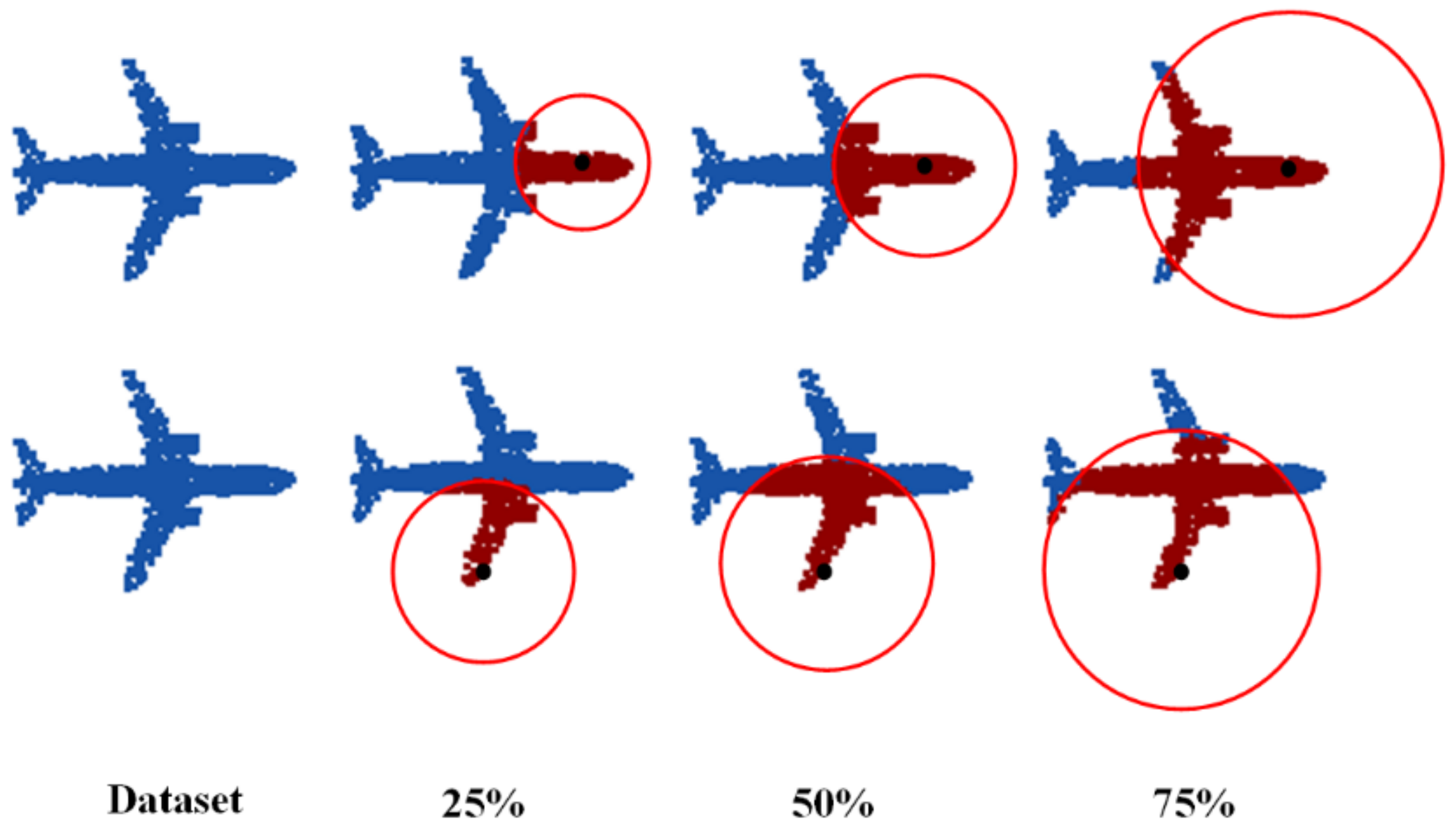
The PP-Net can encode the multi-directional projection of an incomplete point cloud as a 1792-dimensional feature, which represents the global feature of the 3D shape and multi-directional boundary feature. To verify its robustness for point cloud completion with different degrees of missing areas, the network parameters were adjusted to train it to repair point clouds with missing degrees of 25%, 50%, and 75%. Figure 7 and

Table 2. Pred→GT/GT→Pred error of the missing point cloud obtained using the PP-Net. The incomplete point cloud loses 25%, 50%, and 75%, respectively, compared to the original point cloud.

Missing Ratio	$25\%$	$50\%$	$75\%$
Airplane	0.973/0.951	0.962/0.968	0.996/0.989
Guitar	0.459/0.477	0.452/0.486	0.473/0.495

show the performance of the network in the test set. Figure 7 shows that, even in the case of a large missing area, the network can still fully identify and repair the outline of the overall point cloud. Table 2 show that, for predicted point clouds generated with different degrees of missing areas, the error between the predicted point cloud and ground truth is unchanged, which proves the robustness of the proposed network to varying degrees of missing information. To further prove the robustness of the network, the network was trained to complete missing point clouds at multiple locations. The results are shown in Figure 8. The network can still correctly predict the missing point cloud, while ensuring that the error is unchanged.

3.4. Comparison with Other Methods

To verify the advanced nature of the proposed method, in this study, three existing strong baseline point cloud completion methods were selected for comparison with the PP-Net. These three methods are the same as those in the PP-Net. The network was trained based on an encoding–decoding structure. All methods were trained and tested using the same dataset for a quantitative comparative analysis.

L-GAN [37]: L-GAN is the first point cloud completion method based on deep learning, which also uses an encoder–decoder structure, specifically, a PointNet-based encoder and simple fully connected decoder in the decoding module.

PCN [39]: This is the most well-known method for point cloud completion. It provides good results, and is one of the best performing methods for point cloud completion. Similar to the PP-Net, PCN uses an FBD to output the final result.

PF-Net [36]: PF-Net employs a CMLP based on PointNet, which concatenates the features extracted by MLP to obtain the feature vector. The encoder of the PP-Net is inspired by the CMLP. It proposes a three-stage point cloud completion method from rough to fine in the decoding module.

The results are presented in

Table 3. Point cloud completion results of missing areas. The training data comprise 13 different types of objects. The numbers displayed from left to right are Pred→GT/GT→Pred error, which are all multiplied by 1000. The last line represents the overall average error.

Category	L-GAN [37]	PCN [39]	PF-Net [36]	PP-Net
Airplane	3.342/1.205	4.936/1.278	1.121/1.076	1.091/1.072
Bag	5.642/5.478	3.124/4.484	3.957/3.867	4.414/3.466
Cap	8.935/4.628	7.159/4.365	5.295/4.812	6.898/4.237
Car	4.653/2.634	2.673/2.245	2.495/1.840	2.238/1.812
Chair	7.246/2.372	3.835/2.317	2.093/1.955	2.232/2.046
Guitar	0.895/0.565	1.395/0.665	0.473/0.458	0.484/0.551
Lamp	8.534/3.715	10.37/7.256	5.237/3.611	4.222/3.799
Laptop	7.325/1.538	3.105/1.346	1.242/1.067	1.134/1.063
Motorbike	4.824/2.172	4.975/1.984	2.253/1.898	1.897/1.865
Mug	6.274/4.825	3.574/3.620	3.067/3.175	3.078/3.763
Pistol	4.075/1.538	4.739/1.479	1.268/1.067	1.046/1.051
Skateboard	5.736/1.586	3.069/1.784	1.131/1.335	1.043/1.232
Table	2.567/2.578	2.638/2.589	2.376/2.025	2.073/2.211
Mean	5.388/2.679	4.276/2.724	2.469/2.168	2.455/2.166

. Comparing the results of 13 different categories of different objects of point cloud completion, the proposed method (PP-Net) outperforms the existing methods in 6 of the 13 categories for the Pred→GT and GT→Pred errors, namely, airplane, car, laptop, motorbike, pistol, and skateboard. One of the Pred→GT and GT→Pred errors for PP-Net is better than those for the existing methods in four categories: cap, bag, table, and lamp. There are also three types of completion results that are not dominant, namely, chair, guitar, and mug. It can be found that the completion result is mainly affected by the following three factors: (1) whether object is symmetrical, (2) whether there are subtle fine structures, and (3) whether there is occlusion. The PP-Net projects the point cloud in various directions; for symmetrical objects, the missing structure can be inferred from the projection. Objects, such as airplanes, cars, laptops, motorbikes, pistols, and skateboards, are symmetrical in at least one direction, meaning good results can be obtained. The shape of a guitar with a sound hole is not necessarily symmetrical, thus affecting the completion result. The decoder of the PP-Net is based on a folding decoder. It is difficult to deform the grid into subtle, fine structures; because such structures exist in bag, table, chair, and mug, the completion is affected. The disadvantage of the multi-view-based method is that information loss is inevitable when projecting complex structures. Most lamps are equipped with lampshades. During projection, the structural information of the lamp cannot be extracted, thus affecting the completion result. However, in general, the PP-Net achieved better results in some categories, while demonstrating advantages in the average error of all categories.

In Figure 9, the output point cloud generated by the abovementioned methods is visualized, and all were from the test set. Compared with other methods, the PP-Net prediction shows a clear boundary, with a more complete recovery level and finer profile. In (1), (5), and (9), the outputs of the other methods are blurred in the fine profile. In (3) and (8), the outputs of the other methods fail to generate a reasonable shape. In (6), (7), and (8), there is a certain deviation in the outline of the other methods. We also take advantage of PF-Net. Only the missing parts are output, and the hollows and backrests are properly filled in (2) and (4). To summarize, the proposed approach focuses more on boundaries and produces finer profiles.

4. Discussion

This section discusses three sets of comparative experiments designed to analyze some of the design of the network structure: (1) comparison between using and not using boundary extraction, (2) comparison of grid point folding and projection folding, and (3) comparison of using joint loss and only using CD loss between two point clouds.

4.1. Boundary Extraction Analysis

In the projection boundary extraction module, a new boundary extraction algorithm is proposed to extract the boundary points that can reduce the computational cost, while retaining the boundary information of the point cloud, and make the point cloud focus on the structural features. To prove that the proposed method is effective, the boundary extraction module was removed and the projection was directly input into the encoder. The generated result was then compared with the boundary extraction result. The results are shown in Figure 10. It can be seen that the points in the upper half of the red box are dense; these points represent the borders of the chair. As shown in Figure 3d, the borders are more likely to overlap during the projection. The uneven distribution of points when extracting features leads to an uneven distribution of points when generating results. In the lower part of the red frame, a part of the chair legs was not generated. Through comparison, it can be concluded that boundary extraction makes the network focus on the boundary features, while eliminating the influence of overlap. A quantitative comparative experiment was performed on chairs, and the results are shown in

Table 4. Pred→GT and GT→Pred error obtained via boundary and projection as encoder input.

Method	Boundary	Projection
Pred→GT/GT→Pred errors	2.014/1.755	2.347/2.228

. Here, the boundary extraction method has significantly optimized the error of the results, which proves the effectiveness of boundary extraction.

4.2. Plane Folding Analysis

Both folding and PCN adopt a strategy of forcing the concatenation of 2D point grid features. By visualizing the experimental results, it was found that the edge of the generated point cloud geometry was extremely smooth when using these methods. In fact, the original idea of the PP-Net is to use a point cloud projection for folding. Quantitative comparison experiments were performed on chairs; one of which was folded with grid points, and the other was folded with projection. The results are listed in

Table 5. Pred→GT and GT→Pred error obtained via grid point and projection as decoder input.

Method	Grid Point	Projection
Pred→GT/GT→Pred errors	2.014/1.755	1.974/1.804

. Notably, the GT→Pred error using grid point folding is smaller, implying that the completion point cloud covers the ground truth to a higher degree, because of the grid points being folded from the entire plane and the coverage being wider. The Pred→GT error using projection folding is smaller, and represents the difference between the predicted point cloud and real point cloud. Because the projection records the profile information of the point cloud, it can generate a predicted point cloud closer to the real point cloud. Although analyzed from a quantitative perspective, the results generated by the two are almost the same in sum, except for that from the analysis of the visualization effect; the results are shown in Figure 11. Compared with the projection, the distribution of the point cloud generated based on 2D grid point folding is uniform in the red box. The experimental results show that concatenating the features of a 2D point grid can improve the quality of the completed point cloud.

4.3. Loss Function Analysis

The PP-Net uses a joint loss function that combines multi-directional projection distance loss and adversarial loss to optimize network parameters, making the profile of the point cloud finer and closer to the ground truth. To prove that the method is effective, the conventional CD loss function was used between two point clouds for comparison; the results are shown in Figure 12. It can be seen that, without the constraints of multi-directional projection distance loss and adversarial loss, the edge of the point cloud in the red box is blurred. Quantitative comparative experiments were performed on chairs; one of which used joint loss, and the other used conventional loss. The results are listed in

Table 6. Pred→GT error and GT→Pred error obtained via joint loss and CD loss as loss function.

Method	Joint Loss	CD Loss
Pred→GT error/GT→Pred error	2.014/1.755	2.296/1.763

. It can be seen that the joint loss mainly optimizes Pred→GT error, which represents the difference between the predicted point cloud and ground truth. Because the joint loss includes multi-directional projection loss and adversarial loss, the multi-directional projection loss makes the profile of the predicted point cloud closer to the true value, and the adversarial loss makes the predicted point cloud more realistic, both of which optimize the predicted point cloud, thus reducing the Pred→ GT error.

5. Conclusions

This study proposes a new network, PP-Net, to accomplish the task of point cloud shape completion. It directly processes the raw input point cloud with a certain noise without any voxelization or structural assumption. The PP-Net uses a multi-view-based method to directly generate fine point clouds through projections in various directions of the point cloud. The method based on multi-view projection combines global features and multi-directional boundary features to input into the encoder. The MRE of the PP-Net can extract low-, medium-, and high-level features. For the decoder, the PP-Net uses a folding operation to make the distribution of the generated point cloud more uniform. Further, the combination of multi-directional projection distance loss and adversarial loss is used to guide the continuous optimization of the network; finally, a more realistic point cloud with fine profiles is obtained. The experimental results showed that the PP-Net achieved good results and is robust to the lack of different positions and different degrees of incompleteness. The good effect of PP-Net in many categories shows its wide applicability in the field of remote sensing, such as the repair and completion of photogrammetric models in urban basic information mapping and the optimization of 3D shapes in the construction of smart city databases.

However, the completion network is occasionally unable to recover these subtle fine structures. Potential reasons for this are that these structures have small surface areas; this makes the feature extraction more difficult for the encoder, and makes it difficult for the decoder to deform a 2D grid into subtle fine structures. Future work will need to consider methods for improving the feature extraction of these fine structures by combining their local geometric features.

References

1. Liu, H.; Ye, Q.; Wang, H.; Chen, L.; Yang, J. A Precise and Robust Segmentation-Based Lidar Localization System for Automated Urban Driving. Remote Sens. 2019, 11, 1348. [Google Scholar] [CrossRef] [Green Version]
2. Jing, Z.; Guan, H.; Zhao, P.; Li, D.; Yu, Y.; Zang, Y.; Wang, H.; Li, J. Multispectral LiDAR Point Cloud Classification Using SE-PointNet++. Remote Sens. 2021, 13, 2516. [Google Scholar] [CrossRef]
3. Wan, J.; Xie, Z.; Xu, Y.; Zeng, Z.; Yuan, D.; Qiu, Q. DGANet: A Dilated Graph Attention-Based Network for Local Feature Extraction on 3D Point Clouds. Remote Sens. 2021, 13, 3484. [Google Scholar] [CrossRef]
4. Lundell, J.; Verdoja, F.; Kyrki, V. Beyond Top-Grasps Through Scene Completion. In Proceedings of the 2020 IEEE International Conference on Robotics and Automation (ICRA), Paris, France, 31 May–31 August 2020; pp. 545–551. [Google Scholar]
5. Lundell, J.; Verdoja, F.; Kyrki, V. Robust Grasp Planning Over Uncertain Shape Completions. In Proceedings of the 2019 IEEE/RSJ International Conference on Intelligent Robots and Systems (IROS), Macau, China, 4–8 November 2019; pp. 1526–1532. [Google Scholar]
6. Varley, J.; DeChant, C.; Richardson, A.; Ruales, J.; Allen, P. Shape Completion Enabled Robotic Grasping. In Proceedings of the 2017 IEEE/RSJ International Conference on Intelligent Robots and Systems (IROS), Vancouver, BC, Canada, 24–28 September 2017; pp. 2442–2447. [Google Scholar]
7. Mayuku, O.; Surgenor, B.W.; Marshall, J.A. A Self-Supervised near-to-Far Approach for Terrain-Adaptive off-Road Autonomous Driving. In Proceedings of the 2021 IEEE International Conference on Robotics and Automation (ICRA), Xi’an, China, 30 May–5 June 2021. [Google Scholar]
8. Wang, P.; Liu, D.; Chen, J.; Li, H.; Chan, C.-Y. Decision Making for Autonomous Driving via Augmented Adversarial Inverse Reinforcement Learning. In Proceedings of the 2021 IEEE International Conference on Robotics and Automation (ICRA), Xi’an, China, 30 May–5 June 2021. [Google Scholar]
9. Wei, B.; Ren, M.; Zeng, W.; Liang, M.; Yang, B.; Urtasun, R. Perceive, Attend, and Drive: Learning Spatial Attention for Safe Self-Driving. In Proceedings of the 2021 IEEE International Conference on Robotics and Automation (ICRA), Xi’an, China, 30 May–5 June 2021. [Google Scholar]
10. Rad, M.; Lepetit, V. BB8: A Scalable, Accurate, Robust to Partial Occlusion Method for Predicting the 3D Poses of Challenging Objects Without Using Depth. In Proceedings of the IEEE International Conference on Computer Vision, Venice, Italy, 20–29 October 2017; pp. 3828–3836. [Google Scholar]
11. Tekin, B.; Sinha, S.N.; Fua, P. Real-Time Seamless Single Shot 6D Object Pose Prediction. In Proceedings of the IEEE Conference on Computer Vision and Pattern Recognition, Salt Lake City, UT, USA, 18–22 June 2018; pp. 292–301. [Google Scholar]
12. Kehl, W.; Manhardt, F.; Tombari, F.; Ilic, S.; Navab, N. SSD-6D: Making RGB-Based 3D Detection and 6D Pose Estimation Great Again. In Proceedings of the IEEE International Conference on Computer Vision, Venice, Italy, 20–29 October 2017; pp. 1521–1529. [Google Scholar]
13. Sipiran, I.; Gregor, R.; Schreck, T. Approximate Symmetry Detection in Partial 3D Meshes. Comput. Graph. Forum 2014, 33, 131–140. [Google Scholar] [CrossRef] [Green Version]
14. Sung, M.; Kim, V.G.; Angst, R.; Guibas, L. Data-Driven Structural Priors for Shape Completion. ACM Trans. Graph. 2015, 34, 175. [Google Scholar] [CrossRef]
15. Thrun, S.; Wegbreit, B. Shape from Symmetry. In Proceedings of the Tenth IEEE International Conference on Computer Vision (ICCV’05) Volume 1, Beijing, China, 17–21 October 2005; pp. 1824–1831. [Google Scholar]
16. Nguyen, D.T.; Hua, B.-S.; Tran, K.; Pham, Q.-H.; Yeung, S.-K. A Field Model for Repairing 3D Shapes. In Proceedings of the IEEE Conference on Computer Vision and Pattern Recognition, Las Vegas, NV, USA, 26 June–1 July 2016; pp. 5676–5684. [Google Scholar]
17. Zhao, W.; Gao, S.; Lin, H. A Robust Hole-Filling Algorithm for Triangular Mesh. Vis. Comput. 2007, 23, 987–997. [Google Scholar] [CrossRef]
18. Sorkine, O.; Cohen-Or, D. Least-Squares Meshes. In Proceedings of the Proceedings Shape Modeling Applications, Genova, Italy, 7–9 June 2004; pp. 191–199. [Google Scholar]
19. Gupta, S.; Arbelaez, P.; Girshick, R.; Malik, J. Aligning 3D Models to RGB-D Images of Cluttered Scenes. In Proceedings of the IEEE Conference on Computer Vision and Pattern Recognition, Boston, MA, USA, 7–12 June 2015; pp. 4731–4740. [Google Scholar]
20. Xu, Y.; Xie, Z.; Chen, Z.; Xie, M. Measuring the similarity between multipolygons using convex hulls and position graphs. Int. J. Geogr. Inf. Sci. 2021, 35, 847–868. [Google Scholar] [CrossRef]
21. Pauly, M.; Mitra, N.J.; Giesen, J.; Gross, M.; Guibas, L.J. Example-Based 3D Scan Completion. In Proceedings of the Proceedings of the third Eurographics symposium on Geometry processing, Vienna Austria, 4–6 July 2005; Eurographics Association: Goslar, Germany, 2005; p. 23. [Google Scholar]
22. Wu, Z.; Song, S.; Khosla, A.; Yu, F.; Zhang, L.; Tang, X.; Xiao, J. 3D ShapeNets: A Deep Representation for Volumetric Shapes. In Proceedings of the Proceedings of the Eurographics Symposium on Geometry Processing, Graz, Austria, 6–8 July 2015; Eurographics Association: Goslar, Germany, 2015; pp. 1912–1920. [Google Scholar]
23. Chang, A.X.; Funkhouser, T.; Guibas, L.; Hanrahan, P.; Huang, Q.; Li, Z.; Savarese, S.; Savva, M.; Song, S.; Su, H.; et al. ShapeNet: An Information-Rich 3D Model Repository. arXiv 2015, arXiv:1512.03012 [cs]. [Google Scholar]
24. Yang, B.; Wen, H.; Wang, S.; Clark, R.; Markham, A.; Trigoni, N. 3D Object Reconstruction from a Single Depth View with Adversarial Learning. In Proceedings of the IEEE International Conference on Computer Vision Workshops, Venice, Italy, 22–29 October 2017; pp. 679–688. [Google Scholar]
25. Yu, C.; Wang, Y. 3D-Scene-GAN: Three-dimensional Scene Reconstruction with Generative Adversarial Networks. February 2018. Available online: https://openreview.net/forum?id=SkNEsmJwf (accessed on 2 December 2021).
26. Pathak, D.; Krahenbuhl, P.; Donahue, J.; Darrell, T.; Efros, A.A. Context Encoders: Feature Learning by Inpainting. In Proceedings of the IEEE Conference on Computer Vision and Pattern Recognition, Las Vegas, NV, USA, 26 June–1 July 2016; pp. 2536–2544. [Google Scholar]
27. Lin, T.-Y.; Dollar, P.; Girshick, R.; He, K.; Hariharan, B.; Belongie, S. Feature Pyramid Networks for Object Detection. In Proceedings of the IEEE Conference on Computer Vision and Pattern Recognition, Honolulu, HI, USA, 21–26 July 2017; pp. 2117–2125. [Google Scholar]
28. Feng, Y.; You, H.; Zhang, Z.; Ji, R.; Gao, Y. Hypergraph Neural Networks. In Proceedings of the AAAI Conference on Artificial Intelligence, Honolulu, HI, USA, 27 January–1 February 2019; Volume 33, pp. 3558–3565. [Google Scholar] [CrossRef] [Green Version]
29. Liu, Y.; Fan, B.; Xiang, S.; Pan, C. Relation-Shape Convolutional Neural Network for Point Cloud Analysis. In Proceedings of the IEEE/CVF Conference on Computer Vision and Pattern Recognition, Long Beach, CA, USA, 15–20 June 2019; pp. 8895–8904. [Google Scholar]
30. Kanezaki, A.; Matsushita, Y.; Nishida, Y. RotationNet: Joint Object Categorization and Pose Estimation Using Multiviews From Unsupervised Viewpoints. In Proceedings of the IEEE Conference on Computer Vision and Pattern Recognition, Salt Lake City, UT, USA, 18–22 June 2018; pp. 5010–5019. [Google Scholar]
31. He, X.; Zhou, Y.; Zhou, Z.; Bai, S.; Bai, X. Triplet-Center Loss for Multi-View 3D Object Retrieval. In Proceedings of the IEEE Conference on Computer Vision and Pattern Recognition, Salt Lake City, UT, USA, 18–22 June 2018; pp. 1945–1954. [Google Scholar]
32. Dai, A.; Ruizhongtai Qi, C.; Niessner, M. Shape Completion Using 3D-Encoder-Predictor CNNs and Shape Synthesis. In Proceedings of the IEEE Conference on Computer Vision and Pattern Recognition, Honolulu, HI, USA, 21–26 July 2017; pp. 5868–5877. [Google Scholar]
33. Wang, W.; Huang, Q.; You, S.; Yang, C.; Neumann, U. Shape Inpainting Using 3D Generative Adversarial Network and Recurrent Convolutional Networks. In Proceedings of the IEEE International Conference on Computer Vision, Venice, Italy, 22–29 October 2017; pp. 2298–2306. [Google Scholar]
34. Qi, C.R.; Su, H.; Mo, K.; Guibas, L.J. PointNet: Deep Learning on Point Sets for 3D Classification and Segmentation. In Proceedings of the IEEE Conference on Computer Vision and Pattern Recognition, Honolulu, HI, USA, 21–26 July 2017; pp. 652–660. [Google Scholar]
35. Qi, C.R.; Yi, L.; Su, H.; Guibas, L.J. PointNet++: Deep Hierarchical Feature Learning on Point Sets in a Metric Space. arXiv 2017, arXiv:1706.02413. [Google Scholar]
36. Huang, Z.; Yu, Y.; Xu, J.; Ni, F.; Le, X. PF-Net: Point Fractal Network for 3D Point Cloud Completion. In Proceedings of the IEEE/CVF Conference on Computer Vision and Pattern Recognition, Seattle, WA, USA, 13–19 June 2020; pp. 7662–7670. [Google Scholar]
37. Achlioptas, P.; Diamanti, O.; Mitliagkas, I.; Guibas, L. Learning Representations and Generative Models for 3D Point Clouds. In Proceedings of the 35th International Conference on Machine Learning, Stockholm, Sweden, 10–15 July 2018; pp. 40–49. [Google Scholar]
38. Luo, J.; Xu, Y.; Tang, C.; Lv, J. Learning Inverse Mapping by AutoEncoder Based Generative Adversarial Nets. In Proceedings of the International Conference on Neural Information Processing, Guangzhou, China, 14–18 November 2017; Liu, D., Xie, S., Li, Y., Zhao, D., El-Alfy, E.-S.M., Eds.; Springer International Publishing: Cham, Germany, 2017; pp. 207–216. [Google Scholar]
39. Yuan, W.; Khot, T.; Held, D.; Mertz, C.; Hebert, M. PCN: Point Completion Network. In Proceedings of the 2018 International Conference on 3D Vision (3DV), Verona, Italy, 5–8 September 2018; pp. 728–737. [Google Scholar]
40. Sarmad, M.; Lee, H.J.; Kim, Y.M. RL-GAN-Net: A Reinforcement Learning Agent Controlled GAN Network for Real-Time Point Cloud Shape Completion. In Proceedings of the IEEE/CVF Conference on Computer Vision and Pattern Recognition, Long Beach, CA, USA, 15–20 June 2019; pp. 5898–5907. [Google Scholar]
41. Goodfellow, I.; Pouget-Abadie, J.; Mirza, M.; Xu, B.; Warde-Farley, D.; Ozair, S.; Courville, A.; Bengio, Y. Generative Adversarial Nets. In Proceedings of the Advances in Neural Information Processing Systems, Montreal, QC, Canada, 8–13 December 2014; Curran Associates, Inc.: Red Hook, NY, USA, 2014; Volume 27. [Google Scholar]
42. Su, H.; Maji, S.; Kalogerakis, E.; Learned-Miller, E. Multi-View Convolutional Neural Networks for 3D Shape Recognition. In Proceedings of the IEEE International Conference on Computer Vision, Las Condes, Chile, 11–18 December 2015; pp. 945–953. [Google Scholar]
43. Yu, T.; Meng, J.; Yuan, J. Multi-View Harmonized Bilinear Network for 3D Object Recognition. In Proceedings of the IEEE Conference on Computer Vision and Pattern Recognition, Salt Lake City, UT, USA, 18–22 June 2018; pp. 186–194. [Google Scholar]
44. Feng, Y.; Zhang, Z.; Zhao, X.; Ji, R.; Gao, Y. GVCNN: Group-View Convolutional Neural Networks for 3D Shape Recognition. In Proceedings of the IEEE Conference on Computer Vision and Pattern Recognition, Salt Lake City, UT, USA, 18–22 June 2018; pp. 264–272. [Google Scholar]
45. Yang, Z.; Wang, L. Learning Relationships for Multi-View 3D Object Recognition. In Proceedings of the IEEE/CVF International Conference on Computer Vision, Seoul, Korea, 27 October–2 November 2019; pp. 7505–7514. [Google Scholar]
46. Qi, C.R.; Su, H.; Niessner, M.; Dai, A.; Yan, M.; Guibas, L.J. Volumetric and Multi-View CNNs for Object Classification on 3D Data. In Proceedings of the IEEE Conference on Computer Vision and Pattern Recognition, Las Vegas, NV, USA, 26 June–1 July 2016; pp. 5648–5656. [Google Scholar]
47. Wei, X.; Yu, R.; Sun, J. View-GCN: View-Based Graph Convolutional Network for 3D Shape Analysis. In Proceedings of the IEEE/CVF Conference on Computer Vision and Pattern Recognition, Seattle, WA, USA, 13–19 June 2020; pp. 1850–1859. [Google Scholar]
48. Yang, Y.; Feng, C.; Shen, Y.; Tian, D. FoldingNet: Point Cloud Auto-Encoder via Deep Grid Deformation. In Proceedings of the IEEE Conference on Computer Vision and Pattern Recognition, Salt Lake City, UT, USA, 18–22 June 2018; pp. 206–215. [Google Scholar]
49. Fan, H.; Su, H.; Guibas, L.J. A Point Set Generation Network for 3D Object Reconstruction From a Single Image. In Proceedings of the IEEE Conference on Computer Vision and Pattern Recognition, Honolulu, HI, USA, 21–26 July 2017; pp. 605–613. [Google Scholar]
50. Gadelha, M.; Wang, R.; Maji, S. Multiresolution Tree Networks for 3D Point Cloud Processing. In Proceedings of the European Conference on Computer Vision, Munich, Germany, 14–18 September 2018; pp. 103–118. [Google Scholar]
51. Lin, C.-H.; Kong, C.; Lucey, S. Learning Efficient Point Cloud Generation for Dense 3D Object Reconstruction. In Proceedings of the AAAI Conference on Artificial Intelligence, New Orleans, LA, USA, 2–7 February 2018; Volume 32. [Google Scholar]
Figure 1. The process of generating incomplete point cloud data, where the random center point is at the center of the circle.
Remotesensing 13 04917 g001
Figure 2. PP-Net architecture. In the PBE module (Section 2.3), the point cloud is projected to different directions (indicated in red). The boundary extraction method is used to extract the projected boundary feature points (indicated in yellow). After generating the predicted point cloud (indicated in blue), the point cloud is projected in multiple different directions (indicated in red). Then, the CD errors of both the point cloud and projection are calculated (Section 2.6).
Remotesensing 13 04917 g002
Figure 3. Projection transformation and boundary extraction. (a) Projection transformation projects the point cloud (indicated in red) onto three planes (indicated in blue). (b) Boundary extraction algorithm extracts the number of neighbors around each point (indicated in black). A group of points with the least number of adjacencies is selected as boundary feature points (indicated in blue). (ce) Projection transformation and boundary extraction of the point cloud (indicated in blue) in a certain direction (indicated in red).
Remotesensing 13 04917 g003
Figure 4. Structure of the proposed CMLP.
Remotesensing 13 04917 g004
Figure 5. Details of the FBD. First, input the feature vector into the MLP to obtain the codeword used for the folding operation. Then, concatenate the codeword and 2D grid points to obtain the predicted point cloud after two consecutive folding operations.
Remotesensing 13 04917 g005
Figure 6. Visualization of partial point cloud completion results. “Input” represents the input incomplete point cloud, “PP_Net” represents the completion result of the network, and “GT” represents the ground truth.
Remotesensing 13 04917 g006
Figure 7. Examples of repairing results when the input has different extents of incomplete data. (1), (2), and (3) lose 25%, 50%, and 75% points of the original point cloud, respectively. Blue represents the prediction. Gray denotes the undamaged point cloud.
Remotesensing 13 04917 g007
Figure 8. Examples of repairing results with missing point clouds at multiple locations. (1–3) Blue represents the prediction. Gray denotes the undamaged point cloud.
Remotesensing 13 04917 g008
Figure 9. Comparison of point cloud completion results of other methods and those of the proposed network.
Remotesensing 13 04917 g009
Figure 10. Comparison experiment of boundary extraction methods.
Remotesensing 13 04917 g010
Figure 11. Comparison experiment of plane folding analysis.
Remotesensing 13 04917 g011
Figure 12. Comparison experiment of loss function.
Remotesensing 13 04917 g012