Abstract
Forest structure is a useful proxy for carbon stocks, ecosystem function and species diversity, but it is not well characterised globally. However, Earth observing sensors, operating in various modes, can provide information on different components of forests enabling improved understanding of their structure and variations thereof. The Ice, Cloud and Elevation Satellite (ICESat) Geoscience Laser Altimeter System (GLAS), providing LiDAR footprints from 2003 to 2009 with close to global coverage, can be used to capture elements of forest structure. Here, we evaluate a simple allometric model that relates global forest canopy height (RH100) and canopy density measurements to explain spatial patterns of forest structural properties. The GLA14 data product (version 34) was applied across subdivisions of the World Wildlife Federation ecoregions and their statistical properties were investigated. The allometric model was found to correspond to the ICESat GLAS metrics (median mean squared error, MSE: 0.028; inter-quartile range of MSE: 0.022–0.035). The relationship between canopy height and density was found to vary across biomes, realms and ecoregions, with denser forest regions displaying a greater increase in canopy density values with canopy height, compared to sparser or temperate forests. Furthermore, the single parameter of the allometric model corresponded with the maximum canopy density and maximum height values across the globe. The combination of the single parameter of the allometric model, maximum canopy density and maximum canopy height values have potential application in frameworks that target the retrieval of above-ground biomass and can inform on both species and niche diversity, highlighting areas for conservation, and potentially enabling the characterisation of biophysical drivers of forest structure.
1. Introduction
Forest structure can be defined as the three-dimensional arrangement of tree components (leaves, branches and stems), covering land areas of varying dimension. It provides crucial information on how forest ecosystems function, advancing studies of carbon stocks and fluxes [1]. Forest structure is a key determinant of both species and niche diversity [2], and is an important indicator for conservation priorities [3,4]. However, our knowledge of forest structure on a global scale is limited due to multiple factors, such as the inaccesibility of many remote and dense forests, the inability to directly measure forest structure on regional to global scales and constant changes to forests and land use (e.g., deforestation, agriculture).
Large footprint LiDAR data have been used successfully to estimate elements of forest structure, e.g., canopy height, above-ground biomass, stand volume, canopy density and basal area, across various biomes (e.g., [5,6,7]). The Ice, Cloud and Elevation Satellite (ICESat) Geoscience Laser Altimeter System (GLAS) was a full-waveform LiDAR mission, with the main focus being to measure ice sheet elevation. However, the mission was also able to develop vegetation products which have been used to study forest height and structure across the globe [7,8]. Studies have demonstrated that ICESat GLAS canopy density and height metrics are comparable with both airborne LiDAR and ground data in areas of low topography [6,7]. However, issues can arise in certain conditions (e.g., leaf-off and areas of high topography [9,10,11]). ICESat GLAS metrics have therefore been used to develop products of global or regional forest canopy height [8,12,13] or canopy fractional cover [14] and also to characterise canopy fuel loads [15] or to investigate drivers of forest height [16].
Understanding and defining the canopy density of a forest is complex, given that there is no true canopy density measure from in situ data. In situ estimates of canopy density or cover have been undertaken using densitometer estimation, hemispherical photography [17], or Terrestrial Laser Scanning (TLS) [18]. Canopy density metrics from full-waveform LiDAR have been compared to density metrics from both ground and discrete airborne LiDAR data [1,15,19,20], these studies calculate the canopy density value of the full waveform LiDAR as the ratio between the energy received from the canopy and the total energy returned.
As part of a modelling framework that relates remote sensing observations in the microwave domain to canopy density and height, ICESat GLAS footprints have been evaluated in Sweden to develop a relationship that explains canopy density as a function of canopy height by Santoro et al. [21]. The aim of this study was to investigate if the relationship found in [21] could be extended to landscapes across the globe to gather understanding on variations in forest structure and if they can be characterised with such an allometric model.
2. Materials and Methods
2.1. Datasets
2.1.1. ICESat GLAS
The GLAS LiDAR sensor onboard the ICESat mission carried 3 laser instruments, operating exclusively on three 33 day sub-cycles, covering northern hemisphere spring, summer and autumn [7]. Elliptical footprints of ~70 m diameter were spaced 172 m along track, although their size and ellipticity varied through time [9].
Here, we utilised the GLA14 product (version 34), which provides altimetry data for land surfaces with geodetic, atmospheric and instrument corrections applied. The waveform data were provided in the form of parameters from a multi-Gaussian model which was fitted to the raw waveforms. The waveform for each of the footprints was modelled with up to six Gaussians, as described in Hofton et al. [22]. In addition, extra parameters are provided with the GLA14 product which are suitable for identifying footprints affected by, for example, atmosphere, signal saturation or low signal-to-noise ratio.
2.1.2. Additional Datasets
In order to eliminate any urban or un-vegetated areas, remove any footprints that may be affected by topography and classify the ICESat data by biophysical zones, additional datasets were required.
The European Space Agency’s, Climate Change Initiative (CCI), Land Cover project provides a global land cover map for 2010 [23] based on 300 m MERIS and 1 km SPOT-VEGETATION data. The overall accuracy of this dataset is 76 percent. Despite errors of commission and omission, which mostly affected mosaic classes (classes with multiple vegetation types, e.g., mosaic cropland), this was considered a sufficiantly reliable product that can be used to filter out footprints located in non-vegetated areas. The classes used to remove non-vegetated areas were: 0-no data, 190-urban, 200-bare areas, 202-unconsolidated bare areas, 210-water bodies and 220-permanent snow and ice.
The MODIS Vegetation Continuous Fields (VCF) dataset [24] estimates the percent cover of woody vegetation for 2010. The dataset was generated from monthly composites of 500 m surface reflectance data, and has been validated for various biomes and regions (e.g., [19,25,26,27]). These studies show that the VCF dataset is suitable for estimating tree-cover in the majority of regions, however, in sparsely vegetated areas such as savannas it is less-suitable. In particular, Huang and Seigert [26] and Gao et al. [28] found issues with identification of forest and non-forest in both North China and the Tropics, respectively. Despite these errors of commission we removed any ICESat GLAS footprints that had a VCF < 5.
A digital elevation model (DEM) produced by de Ferranti [29] consists of gap-filled 3 arc-seconds Shuttle Radar Topographic Mission (SRTM) elevations for regions between 60° N and 56° S. Above 60° N, elevations were calculated from multiple datasets (e.g., topographic maps, optical imagery, DEMs) which were selected according to quality for a given region. Further details on the selection process can be found in de Ferranti [29]. Despite some inaccuracies in this dataset, reported by de Ferranti [29], an analysis of other global DEMs by Rizzoli et al. [30] indicates that these show artefacts that could impact the filtering of the GLAS dataset, therefore, the de Ferranti dataset was applied in this study.
2.1.3. World Wildlife Federation Ecoregions
Forest structure and composition are dependent on multiple factors, such as altitude, temperature, precipitation and edaphic conditions [3,31,32]. Dividing the globe into regions of similar forest structure is therefore a complex task. The World Wildlife Federation (WWF) generated ‘ecoregions’ which contain geographically distinct assemblages of species, natural communities or environmental conditions. In addition to precipitation, temperature and spectral signatures from remote sensing, they also incorporated the geological history, the importance of endemic genera and distinct assemblages of species [4]. The definitions and boundaries of the ecoregions are therefore relatively subjective but lay a suitable foundation for an investigation into variations in forest structure. In this product, the world’s land masses are divided into 14 major habitat types, or biomes (Figure 1). These biomes contain 827 ecoregions with a mean area of 164,000 km but ranging from the Sahara desert (4.6 million km) to small island ecoregions of just 6 km.
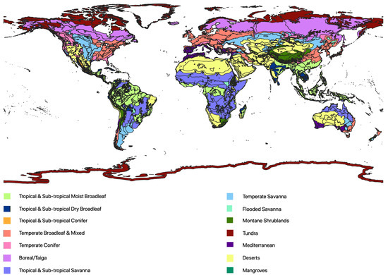
Figure 1.
Map of the distribution of WWF ecoregions categorised by biome (14) adapted from Olsen et al. [4].
2.2. Pre-Processing
Canopy density and canopy height were estimated from ICESat GLAS waveforms by assuming that: i, the ratio between the energy received from the canopy and the total energy returned and ii, RH100, represent canopy density and forest height, respectively [1,15,19,20].
The ICESat GLAS dataset was filtered for various error and noise sources following Los et al. [8] and Simard et al. [12]. As only forest footprints were of interest to this study, footprints: (i) with only one peak (GLAS parameter i_numPk), (ii) with the MODIS VCF < 5 [33] or (iii) categorised as ‘non-vegetated’ with the CCI Land Cover product [23] were also removed. To reduce topographic effects, filtering was computed according to Simard et al. [12], maintaining footprints located on terrain slopes <5 and requiring a correction of slope <25 percent of the RH100 before correction, with slope estimates for each footprint derived from the SRTM DEM [29], although this may not have been sufficient to identify all footprints affected by topography.
For the remaining footprints, canopy height was calculated as the difference between GLA14 parameters SigBegOff and gpCntRngOff (elevation of lowest gaussian peak in the waveform). To estimate the canopy density from ICESat GLAS, the ratio between the energy received from the canopy and the total energy received was calculated using the GLA14 parameters Gamp, Gsigma and gpCntRngOff [15].
The different laser periods were reviewed for consistency. Laser 1 was used for the first 2 cycles (February–March 2003), Laser 2 for the next 5 cycles (September 2003–June 2004) and then Laser 3 for 11 cycles (October 2004–October 2008) before Laser 2 was reinstated for the last 3 cycles (November 2008–October 2009) [34]. A global mean canopy height and mean canopy density was calculated for each of these 4 laser periods. Due to the complexity of seasonal variations in phenology across the globe and the limited footprints between March and November, no leaf-on/leaf-off filtering was applied. Following filtering, ca. 21 million footprints remained (see Supporting Information Figure S1). The combination of the nature of ICESat GLAS imaging and the filtering described above resulted in a heterogeneous footprint distribution: Sub-Saharan Africa and South America have the most available footprints, and East Asia, Australia and mountainous regions have the fewest.
2.3. Methods
This study investigated the extension of the model proposed by Santoro et al. [21] in Swedish forests to explain canopy density (i.e., a variable of horizontal structure) as a function of canopy height (m; i.e., a variable of vertical structure):
In Equation (1), canopy density (CD) is described as a function of canopy height (h) by means of an exponential function, which is characterised by a single parameter, q. This model was selected by Santoro et al. [21] following an analysis of functions fitted to the ICESat GLAS observations, which revealed that the rise-to-max function was the most robust. The analysis undertaken in Sweden demonstrated a spatial variation of the q parameter, with values ranging from approximately 0.04 to 0.10 across the country, which was interpreted as originating from variations in forest composition and structure. A preliminary investigation at coarse scale was also undertaken across other biomes, indicating the potential for Equation (1) to characterise the relationship between the two metrics on a global scale [21].
The ICESat GLAS data were stratified according to the different WWF ecoregions. Potential outliers were removed by calculating the logarithm of RH100 for each ecoregion and trimming the upper and lower 5 percent. A least squares regression, between canopy density and canopy height, was fitted using the scipy [35] Levenberg–Marquardt method to obtain an estimate of the parameter q for each ecoregion. The mean squared error (MSE) between the actual and predicted values of canopy density were also calculated for each regression. Finally, the standard error (SE) of the estimated q-value was calculated using bootstrapping, with 100 iterations per ecoregion. This was undertaken in order to determine the minimum number of footprints required to fit the regression.
WWF ecoregions was originally conceived to contribute towards global conservation exercises, as these describe broad ecologically meaningful areas. However, the product does not capture localised variations within these ecoregions [36]. Over 50 percent of Sweden is dominated by one ecoregion, but the large variation in q seen in Santoro et al. [21] highlights that further subdivision was required. As localised variations within ecoregions are not mapped at a global scale, the subdivision was based on a grid system.
There was a trade off in the area of this subdivision between the ability to capture variations in forest structure whilst ensuring sufficient footprints available for each regression. Therefore, a 1° grid square was selected. A union was generated between the WWF ecoregions and a 1° × 1° grid. Meaning each grid cell was divided by the ecoregions within it and vice versa (see Supporting Information Figure S2). Of the resulting polygons, 37 percent did not have sufficient footprints for a regression (<100, see results). These were removed and the original underlying q-value for the ecoregion was used in place. For each of the remaining new polygons, a q-value, MSE and SE were calculated using the same methods as undertaken initially for the ecoregions.
Global layers of forest canopy height and canopy cover have been developed as they can be used as predictors of above-ground biomass (AGB) or to inform on the delivery of important ecosystem services [12,37,38]. In order to provide further information on forest structure, the means of the top 10 percent of canopy height and canopy density values were calculated, using the ICESat GLAS data for each polygon, after the removal of the potential outliers described above. This provided, for the entire polygon, a representative estimate of ‘maximum’ canopy height and ‘maximum’ canopy density, herein referred to as H and CD, respectively.
3. Results
Comparison of the global mean canopy height for each laser period indicated a drop of over 50 percent for the last phase of Laser 2 compared to the 3 other laser periods (see Supporting Information Table S1). For this reason, laser periods 2D-F were removed from the dataset. Polygons with over 100 footprints had standard errors < 10 percent, whereas lower quantities of footprints presented increasingly higher SE values (see Supporting Information Figure S3). 100 footprints was therefore set as the threshold for including the q-value. This was also the threshold adopted for exclusion of the polygons generated by the union of WWF ecoregions and the 1 × 1 grid.
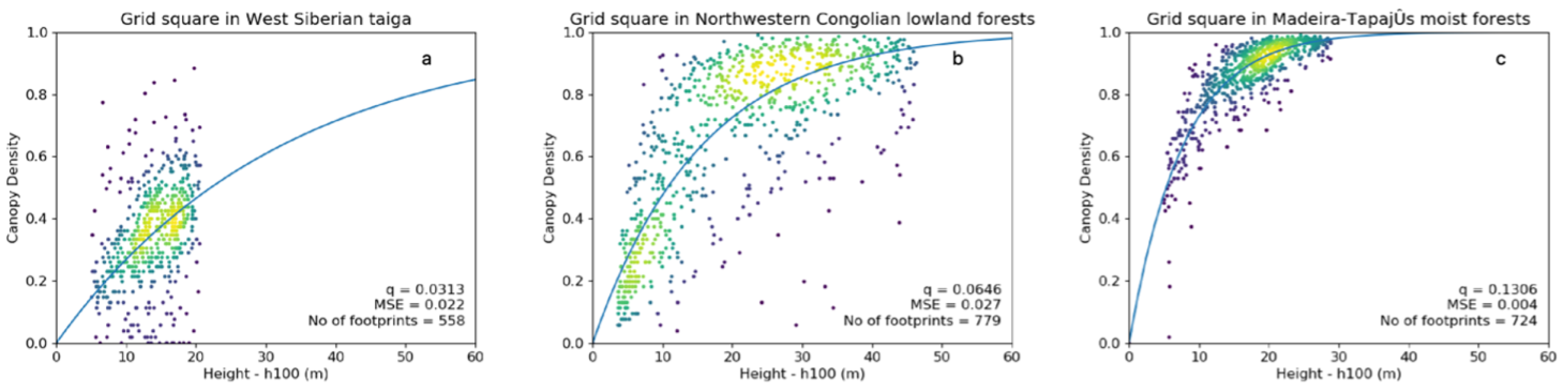
The model described in Equation (1) corresponded with the ICESat GLAS metrics, despite varying patterns of the canopy density to canopy height relationship (Figure 2). The varying dispersion of the data resulted in MSE values with a median of 39 percent and inter-quartile range of 27–60 percent relative to the q-values obtained.
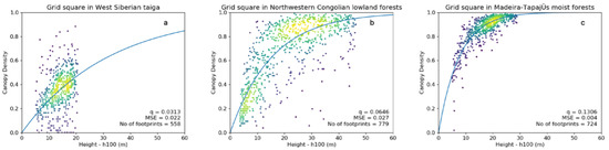
Figure 2.
Least squares regression curves denoted by blue lines (extended to 60 m canopy height for comparison) for the exemplary polygons. With (a) a low q-value (0.031), (b) a q-value close to the global mean (0.064) and (c) a high q-value (0.131). Dots represent ICESat GLAS data as density plots with the viridis colour scale, with yellow being most dense.
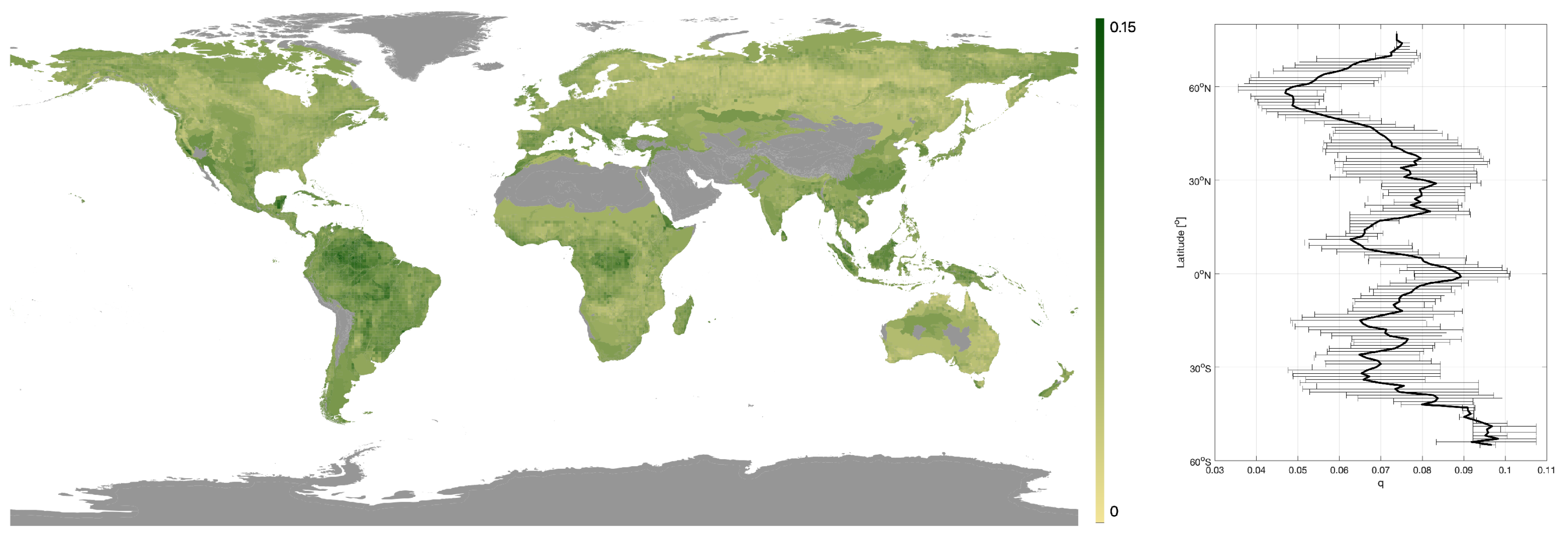
Values of the q parameter ranged from 0.019 to 0.153 across the globe. Higher q-values indicated a rapid increase in canopy density with canopy height and were found in dense tropical forests (means per biome > 0.075), whilst the lowest values (means per biome < 0.055) were associated with the sparser forests in savanna and boreal regions (Figure 3). A latitudinal trend of higher q-values in the tropics to lower values in the pan-boreal regions and continental Australia was observed, although an increase in q-values in the polar regions was noticed, particularly in the southern hemisphere (Patagonia, Tasmania and New Zealand; Figure 3).

Figure 3.
Map of q-values obtained. Grey represents areas with < 100 ICESat footprints. Plus, a latitudinal plot of q-values with the black line denoting the median q-value and the bars the interquartile range.
The division of q-values per biome provided further information on the variation of this canopy height to canopy density relationship across the globe (Figure 4 and see Supporting Information Table S2). At the lower end of the range, q-values for the Boreal/Taiga and Temperate Conifer biomes exhibited similar distributions through ANOVA (p = 0.02), with mean q-values of 0.048 and 0.051, respectively (more than 1 standard deviation from the global mean of 0.064). The three savanna biomes exhibited mean q-values lower than the global mean (0.054–0.062). The Tropical and Sub-Tropical (TST) savanna and TST flooded savanna also displayed similar distributions through ANOVA (p = 0.01). At the upper end of the range, the TST Moist Broadleaf, Mangrove and TST Dry broadleaf had the highest mean q-values (0.076–0.083). Biomes showing large variance in the q-values were the Mediterranean (0.35 × 10), Temperate Savanna (0.30 × 10) and all TST biomes (>0.26 × 10). The Tundra biome and Montane Shrublands stood out with their small variances (0.1 × 10) around means (0.063 and 0.064, respectively) close to the global mean.
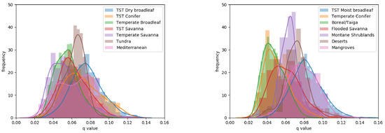
Figure 4.
Histograms of q-values per biome, split into two figures for clarity.
Values of q were found to vary within biomes for each of the different realms (see Supporting Information Table S3). Within the TST Savanna and Temperate Broadleaf biomes, the highest q-values were found in the Neotropics (means of 0.081 and 0.070, respectively), and the lowest in Australasia (means of 0.042 and 0.047, respectively). With the exception of the Mediterranean and Mangrove biomes, the Neotropical realm had the highest mean q-value in every biome. This was particularly noticeable in the TST Moist Broadleaf biome (mean of 0.088) where it is distinguished from the three other realms where means ranged from 0.075 to 0.076. Relatively distinct distributions of q-values per realm were observed for the Mediterranean (mean 0.0046 to 0.077), Flooded Savannas (0.048 to 0.072) and Boreal/Taiga (0.54 and 0.43).
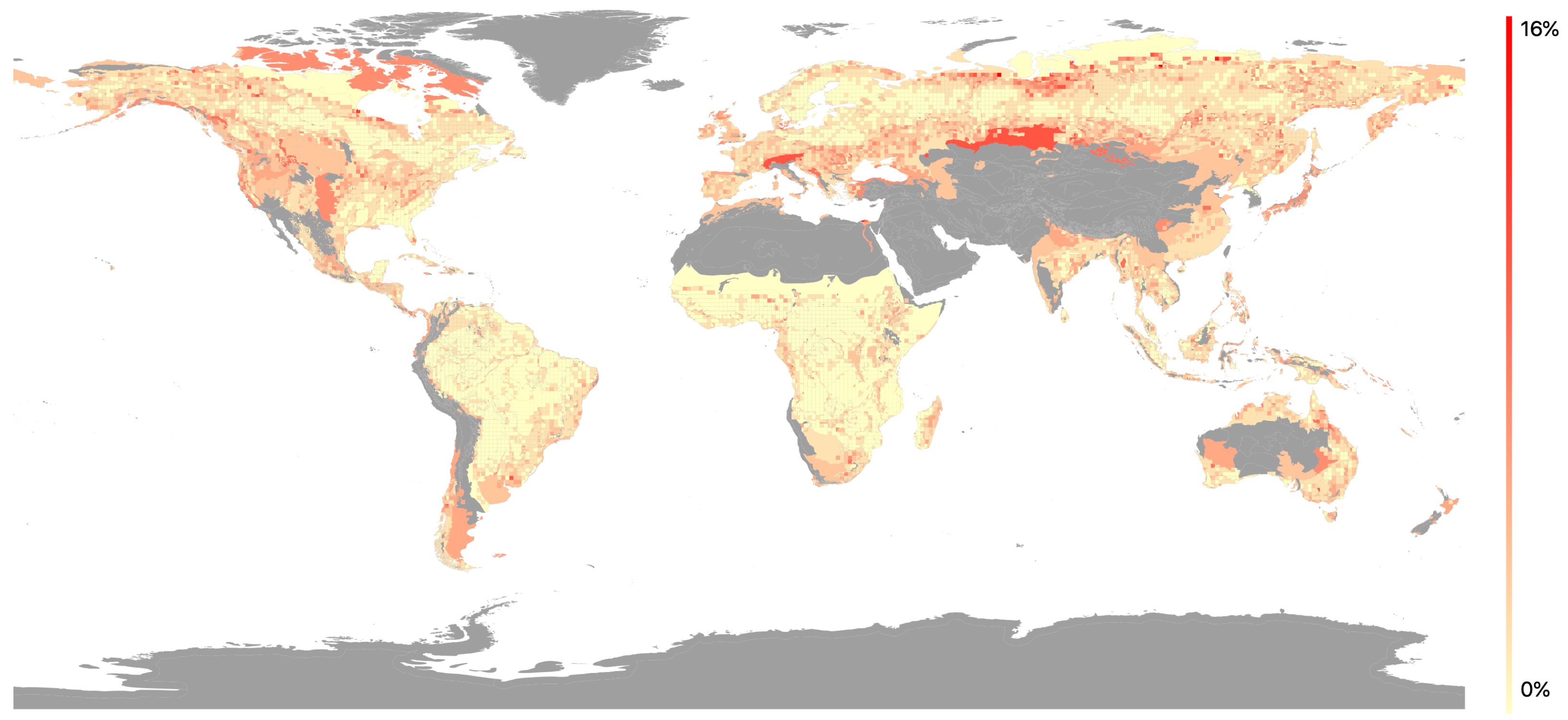
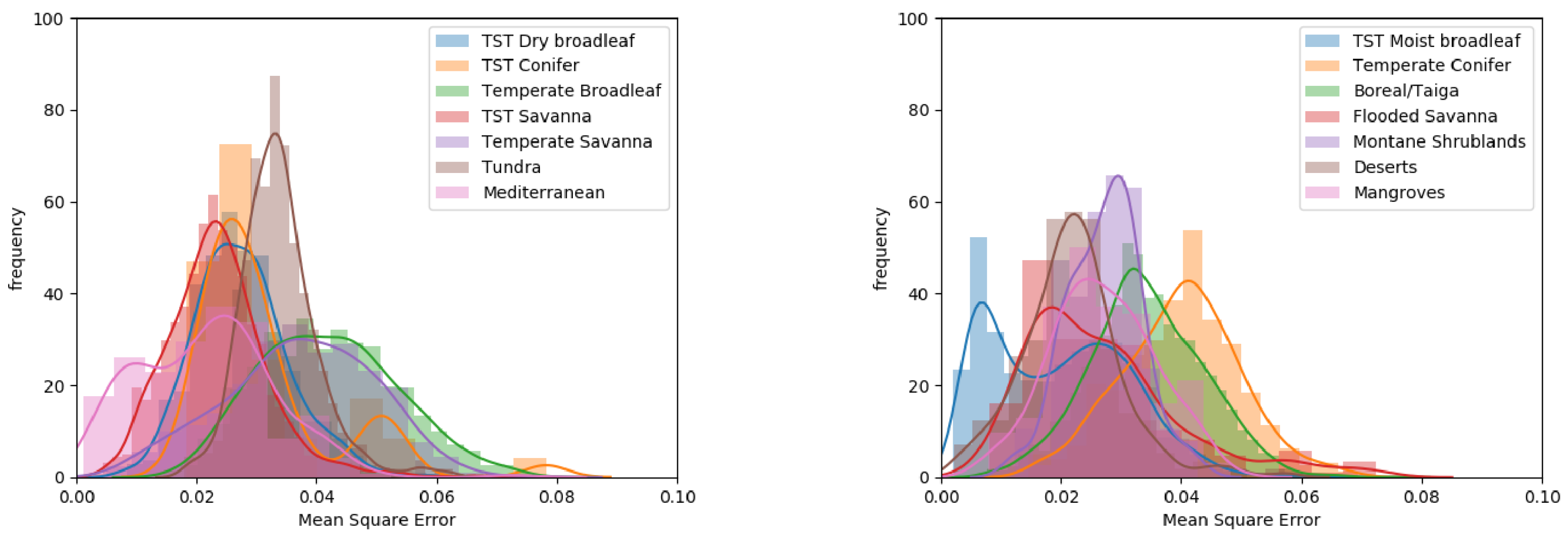
The spatial variation of MSE values indicated that the highest values were in temperate regions across the Northern hemisphere and in Eastern Australia (Figure 5). The lowest values were found in tropical regions. Variations in MSE were observed between biomes (Figure 6), with the three temperate biomes exhibiting the highest mean MSE values (0.037–0.042). Mid-range values (0.026–0.033) were associated with; the TST Dry Broadleaf and TST Conifer biomes found close to the equator; the Flooded Savanna and Mangrove biomes experiencing regular flooding; and the Montane Shrubland and Tundra biomes characterised by extreme temperatures and poor soils. The lowest mean MSE value (0.019) was found in the TST Moist Broadleaf biome. The bi-modal distribution within this biome was related to geographical location: with the high MSE values (0.01–0.02) relating to Amazonia, the Congo Basin and the island of New Guinea, whereas lower MSE values (0.03–0.04) were located in the Indo-Malay realm, south-eastern Brazil, Central America and coastal regions of the Afro-tropics.

Figure 5.
Map of mean squared error (MSE) values (plotted as MSE relative to the q-value in percent) with 1 grid results overlain on the ecoregion results. Areas in grey have no regression due to lack of available footprints.
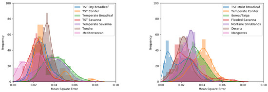
Figure 6.
Frequency distributions of MSE per biome, split into two figures for clarity.
A zonal distribution of q-values was observed when comparing with the CD and H values (Figure 7). The lowest q-values (blue dots) were found in the forests with lower CD values for each H value, or higher H values for each CD value. The highest q-values (pink and brown dots) were found in the forests which reach CD at the lowest H. The tallest, densest forests therefore were not necessarily associated with the highest q-values. For each range of q-values, a distinct pattern of CD and H values was observed. As q increased, these patterns shifted, with CD and H increasing with q until CD values were reached (CD > 0.96). Above this point, there was a trend of decreasing H with increasing q: for CD > 0.96, a negative correlation of q to H was observed (p < 0.01, n = 897).
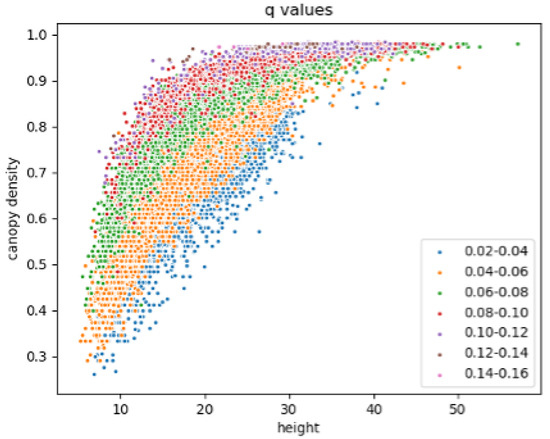
Figure 7.
Maximum canopy height and canopy density values for each 0.02 range of q-values.
Furthermore, in certain biomes, variations in CD and H values were observed for each realm (see Supporting Information Table S3). In the TST Savanna biome, the Neotropical realm had the highest CD values at the lowest H, whereas Australasia had sparser forests for each H value. The Neotropics also demonstrated these high CD values for lower H values in the TST Dry Broadleaf, with the Indo-Malay Realm having generally taller forests for each CD value. The Mediterranean biome had different forest structure characteristics for each realm, with 82 percent of Australasian polygons having a CD < 0.65, whereas the Palearctic had only 6 percent of polygons below 0.65. The Australasian polygons with higher CD values were taller than the Palearctic polygons with similar CD values. In the Desert biome this pattern of low CD in Australasia was again observed. Investigating CD and H values led to further understanding of the q parameter. For example, in the Montane Shrublands and Tundra biomes, low H values were observed (77 percent < 10 m and 90 percent < 15 m, respectively), alongside CD values close to the global mean (means of 0.72 and 0.77, respectively). These canopy density values in relation to canopy height resulted in q-values close to the global mean.
4. Discussion
The model described by Equation (1) was able to capture the relationship between canopy density and height (Figure 2) for biomes across the globe, despite the dispersion of the height and canopy density values in some biomes (particularly temperate). The single parameter (q) of the allometric model captured spatial variations in forest structure and corresponded with CD and H values across the globe (Figure 7). This combination of q, CD and H provided understanding of the development of forest structure in different regions of the globe. For example, a high q-value with low H would indicate dense thickets and shrubs, whereas a similar q-value for higher H would indicate a forest with dense canopy that closes quickly as the forest grows.
Analysis of the SE demonstrated the impact of the number of footprints available for the regression on the precision of the q-value obtained (see Supporting Information Figure S3). The quantity of available footprints is affected by the filtering applied but also influences the selection of layers used to group the ICESat footprints. The nature of the ICESat GLAS imaging pattern and the filtering applied (removal of un-vegetated and mountainous areas) biased the quantity of footprints available for the regression towards areas of continuous forest cover and particularly impacted the quality of the regression in regions of savanna or tundra. The removal of footprints in mountainous areas was inevitable due to the adverse impact of slope on the ICESat data, but this also resulted in the elimination of large areas of natural/semi-natural forest from the analysis (e.g., in Indonesia).
WWF ecoregions were selected as a broad characterisation of multiple biophysical variables that may influence forest structure. However, localised variations of these variables within ecoregions are not available on a global scale. In an attempt to capture some of these localised variations, a 1° grid was applied as a compromise to the number of footprints available for a regression. Analysis of the potential factors contributing to these localised variations indicate that they may be better captured with the use of alternative layers, such as altitude, temperature, precipitation, geology or a wilderness layer. This was not possible in this analysis due to the relatively sparse sampling of ICESat GLAS and the additional filtering applied.
4.1. Biomes
This section investigates the varying patterns of q-values found within and between biomes. Please refer to Supporting Information Table S3 where a distribution map of each biome is provided together with a histogram of q-values per realm and scatterplot of the CD and H values.
Characterised by low variations in annual temperature and high levels of rainfall, with high species richness [39], TST Moist Broadleaf forests are multi-layered and rapidly attain a closed canopy, producing the highest mean and maximum q-values of all biomes (see Supporting Information Table S2). The higher q-values noted in the Neotropics (see Supporting Information Table S3) align with the higher canopy fractional cover values [14] found in this realm and may be attributed to structural differences compared to other realms including a greater quantity of epiphytes (e.g., bromeliads).
TST Dry Broadleaf forests experience warm temperatures year-round and long dry seasons which can last several months. These dry periods cause shedding of the leaves of deciduous trees allowing the development of a thick underbrush as sunlight reaches the understorey [40]. The Neotropics have the most diverse of the TST Dry Broadleaf forests, particularly in southern Mexico and Brazil, which may explain their higher q-values (see Supporting Information Table S3). The Neotropical forests also reach higher CD values at lower H values compared to the other 3 realms (see Supporting Information Table S3). The Indo-Malay realm is characterised by sparser forests in each H range. This may be due to anthropogenic activities—for example, the replacement of the multi-storied native sal (Shorea robusta) native woodlands with teak (Tectona grandis), and the conversion through intensive grazing of habitats into scrub and savanna woodlands [41].
The many small, isolated regions that characterise the TST Conifer biome meant that the majority of the polygons were not included due to a lack of ICESat GLAS footprints. The results for this biome were therefore only representative of Central America. Despite being representative of this limited geographical area, this biome had the largest variance in q-values indicating a wide spread of forest structures in this biome, which may be caused by disturbance regimes such as epizootics, windthrow and fire [42].
The Temperate Broadleaf and Mixed Forests biome displayed a different distribution of q-values for each realm (see Supporting Information Table S3). This may be due to a large number of endemics specific to certain ecoregions. In the frequency distribution of q-values for the Australasian realm (see Supporting Information Table S3) the peak of higher values can be related to pockets of dense forest in Tasmania and on the North Island of New Zealand, whereas the lower values relate to the inclusion of urban and agricultural areas in the human-modified regions of South Eastern Australia. In the Neotropics, the higher q-values (mean of 0.070) may be attributed to the dense understorey of bamboo, ferns and evergreen angiosperms (Arroyo M.T.K. et al., 1996). The highest mean MSE value (0.042) found in this biome was attributed to the effect of phenology described by Pang et al. [9] and the pattern of ICESat GLAS imaging during the northern hemisphere summer. In addition, the higher mean MSE values in the Palearctic and Nearctic realms (0.041 and 0.040, respectively) may be attributable to high levels of anthropogenic activity, with these regions being some of the most densely populated outside of India. MSE values across all realms may also be influenced by high beta diversity (the ratio between regional and local species diversity), with large numbers of local endemics in many ecoregions [43].
Some of the highest levels of forest biomass are found in the Temperate Conifer biome, which consist of species such as pine (Pinus), cedar (Cedrus), fir (Abies) and redwood (Sequoia) with this often leading to the establishment of a distinct overstorey layer and an understorey of grasses, ferns and forbs. The second highest mean MSE in this region (0.039) may again be due to the heterogeneous nature of disturbances such as fire, windthrow and epizootics. Despite the high biomass, this biome has the 2nd lowest mean q-value (0.051) potentially relating to the slow regeneration of late-successional species [44].
The Boreal and Taiga regions are dominated by evergreen (Abies, Picea and Pinus) and deciduous (Larix) needle-leaved species with some deciduous broadleaved trees, mainly Birch (Betula) and Poplar (Populous) [45,46]. The lowest mean q-value found in this biome was attributed to slow regeneration of mature forests and the challenging climatic and edaphic conditions. The higher q-values in the Nearctic compared to the Palearctic may be due to the milder mean annual temperature, and the predominance of Larix in Eastern Siberia which are taller and have sparser canopies than the evergreen species dominating the Canadian ecoregions [47].
The boreal/taiga biome and temperate conifer biomes have matching distributions of q-values through ANOVA (p = 0.02), which may be attributed to the slow regeneration of the coniferous species present in these biomes. However, the effect of the warmer climate on the temperate conifer biome is highlighted when comparing the H and CD values (see Supporting Information Figure S4).
Characterised by low levels of rainfall, between 90 and 150 cm per annum, vegetation composition in the TST Savanna is driven by the variability in soil moisture, fire regimes and herbivory [48]. Each realm has a distinctive pattern of q-value distribution (see Supporting Information Table S3), which is matched by a clear distinction in the patterns of H and CD for each realm (see Supporting Information Table S3). The highest values, found in the Neotropics, relate to the Cerrado and Llanos regions with complex habitats, gallery forests and tropical dry forests. The Afro-tropics are comprised of the miombo and mopane woodlands whereas Australasian TST Savannas consist of eucalypt woodlands with tall but sparse vegetation. The lower q-values and CD values in the Australasian realm may also be related to the greater prevalence crown fires (often of higher severity than the ground fires more prevalent in the Neo- and Afro-tropical realms). Despite these distinctive distributions between realms, within realms the alternative stable states evident in TST Savannas [14,48] were not observed, potentially due to alternative definitions of tropical forest and savannas being used.
The regions of Temperate Savanna are generally treeless landscapes with the exception of riparian or gallery forests along rivers and occasional clusters of trees [49]. The natural flora has largely been replaced by agriculture, which influences both the number of footprints available for the regression and the quality of that regression. The highest q-values (mean of 0.075) found in the Neotropics were driven by Cortaderia selloana (Pampas grasses) and the dense thorny shrubland or ‘espinal’ forests of Argentina. High q-values in the Nearctic were directly linked to the ‘California Central Valley Grasslands’ ecoregion, which is described by intensive agriculture, these q-values therefore relate more to cultivated woody vegetation (e.g., orchards) rather than natural vegetation.
In the Mediterranean biome, the second largest variance and bimodal distribution of q-values, was linked to the difference in the q-values in Australasia compared to the Palearctic (see Supporting Information Table S3). The low CD values in the Australasian Mediterranean related to the mallee regions which are often affected by repeated fires and coppiced growth [50], whereas the increased precipitation supporting the denser and taller forests of the Southwest Australia Woodlands ecoregion [51] was highlighted by higher CD values. In contrast, the Palearctic Mediterranean regions have higher CD values for lower H values.
Characterised by cold temperatures and poor soils, the Montane Shrublands and Tundra regions have low H values, but CD values close to the global mean resulting in q-values close to the global mean. Ninety-seven percent of the Montane Shrublands polygons are located in the Afro-tropics where the triple-canopied forests may explain these canopy density values [52]. In the Tundra biome, the canopy density values are explained by the pockets of subalpine forests of species such as mountain hemlock (Tsuga mertensiana), alpine fir (Abies lasiocarpa), lodgepole pine (Pinus contorta), black and white spruce (Picea glauca and P. mariana) and aspen (Populous tremuloides). As well as the closed forests of Sitka spruce (P. sitchensis) and western hemlock (Tsuga heterophylla) in lower elevations [53].
The highest q-values in the Flooded Savanna biome were found in the Neotropics (mean of 0.072) where the denser forests of the Everglades and the Pantanal are located (see Supporting Information Table S3). The Palearctic has the lowest q-values (mean of 0.048), with the higher values from the realm being found around the Nile delta. The Mangrove biome presented a higher mean q-value (0.079) which was attributed to rapid canopy closure following colonisation and growth.
In the deserts, high temperatures and water availability were limiting but where these were more favourable (e.g., near oases, shaded areas, river-beds), the density of vegetation was greater. The q-values obtained are characteristic of these oases with little variation between each of the realms except in Australasia which has lower CD values relating to vegetation around the billabongs (see Supporting Information Table S3).
4.2. Maximum Canopy Density and Canopy Height Patterns
Height is used as a proxy for biomass in the development of AGB products in many regions of the globe. The distribution of CD and H values varies with the q parameter (Figure 7). The decreasing H values for CD > 0.96 may be due to a saturation of the GLAS signal in dense forests [54], although there may also be an influence of the pattern of canopy density values within the polygon: polygons at the lower range of H for CD 0.96 (e.g., H 30) tend to have canopy density values across the full range of possible values, whereas polygons with higher H values (e.g., H 40) tend to have limited ranges of canopy density values (approx. 0.6–0.98).
Figure 7 and Supporting Information Table S3 demonstrate the variations in the CD values for H values between and within biomes and realms. The CD and H values explained the underlying forest structures influencing the q parameter obtained. For example, across Australasia, low q-values were associated with forests with both low CD and H, whereas in the Palearctic lower q-values were found in forests with low CD values in relation to H values above the global mean.
The pattern of q-value distribution across CD and H values demonstrates how it could be used to inform on forest structure and improve biomass retrieval. Hansen et al. [2] also highlight that structure can be used as a proxy for both species and niche diversity, particularly when coupled with disturbance patterns and maximum potential height and canopy density for given biophysical variables.
Tao et al. [16] applied GLAS data to demonstrate that moisture availability is a key determinant of forest canopy height, with canopy height increasing with P-PET (annual precipitation minus annual potential evapotranspiration) to a peak at approximately 680 mm of P-PET and then decreasing. Similarities were found between q and the P-PET map of [16]: lower q-values in areas of low P-PET (e.g., across Russia and Canada), and increasing q-values with increasing P-PET (e.g., in the tropics, Tasmania, New Zealand and southern Chile). However, q-values did not decrease with P-PET values > 980 mm in the tropics, potentially due to the higher canopy density in these regions [14].
5. Conclusions
Our work investigated the feasibility of applying a simple allometric model to subdivisions of forest canopy height and canopy density metrics from ICESat GLAS LiDAR footprints. The allometric model described in Equation (1) captured variations of forest structure across biomes, realms and ecoregions, with biomes in TST latitudes providing the strongest fit to the model. Densely populated temperate regions (broadleaf, conifer and savanna) with more heterogeneous landscapes were characterised by higher MSE values. The pattern of the relationship between q-values and CD and H values highlights the necessity for considering the effects of both canopy height and canopy density when estimating forest biomass. The combination of q, CD and H also has the potential to inform on both species and niche diversity highlighting areas for conservation and allowing the expansion of the development of a Structural Condition Index by Hansen et al. [2] to a global scale.
Filtering of the ICESat GLAS footprints provided a heterogeneous sampling of the globe. However, sufficient footprints remained across areas of woody vegetation, except in regions with high topography. The combination of WWF ecoregions and a 1 grid does not capture all the factors influencing species composition and growth rates. In particular, no allowance was made for moisture availability, altitude, soil type or anthropogenic influences. Localised variations could not be captured due to the quantity of available footprints for the regression. Investigation into the influence of alternative drivers of the canopy density to canopy height relationship should be possible with NASA’s Global Ecosystem Dynamics Investigation (GEDI) data: the increased quantity of data, denser spatial sampling, smaller footprint dimension and sampling throughout the year will allow for a division into leaf-off and leaf-on data, and potentially reduce the effect of topography and allow more localised drivers to be captured. The ability to use spaceborne LiDAR to capture and model the relationship of canopy height to canopy density across the globe opens opportunities for improvement of AGB mapping and change detection. The European Space Agency’s CCI Biomass project has already incorporated this allometric model into their AGB retrieval algorithm following the methods in Santoro et al. [21].
Supplementary Materials
The following are available at https://www.mdpi.com/article/10.3390/rs13244961/s1, Figure S1: Map of distribution of ICESAT GLAS footprints after filtering, represented as number of footprints per 1o grid square. Areas in grey have no footprints, Figure S2: An ecoregion demonstrating the union generated with the 1o grid. Black dots represent ICESat GLAS footprints for the entire ecoregion. Areas in white use the underlying ecoregion q value which is calculated from all the ICESat GLAS footprints shown. Areas in grey are where the ecoregion has been subdivided by grid square, here the q value has been calculated using only the footprints within that grid square and ecoregion, Figure S3: The influence of the number of footprints per polygon on the Standard error obtained. X axis is limited to 500 footprints for clarity, Figure S4: Maximum canopy density and maximum height values per realm for the Temperate Conifer and Boreal/Taiga biomes, Table S1: Global mean canopy height and canopy density for each laser period of ICESat GLAS. Table S2: Descriptive statistics of the allometric parameter (q) and Mean Squared Error (MSE) for each biome. Table S3: Table with, for each biome: histogram of q values per realm, scatterplot of maximum CD and maximum height per realm and map of distribution per realm. The realm colours are maintained across each row.
Author Contributions
Conceptualisation, M.S.; methodology, M.S. and H.K.; investigation, H.K.; data curation, O.C.; writing—original draft preparation, H.K.; writing—review and editing, all authors; supervision, R.L., P.B. and M.S. All authors have read and agreed to the published version of the manuscript.
Funding
This research has been funded by the European Space Agency (ESA) as part of the CCI Biomass project of the Climate Change Initiative (ESA ESRIN/Contract Number 4000123662).
Institutional Review Board Statement
Not applicable.
Informed Consent Statement
Not applicable.
Data Availability Statement
All the datsets used as part of this analysis can be found in the references. Code is available at: https://github.com/HeatherKmtb/q_research, accessed on 25 November 2021.
Conflicts of Interest
The authors declare no conflict of interest. The funders had no role in the design of the study; in the collection, analyses, or interpretation of data; in the writing of the manuscript, or in the decision to publish the results.
References
- Means, J.E.; Acker, S.A.; Harding, D.J.; Blair, J.B.; Lefsky, M.A.; Cohen, W.B.; Harmon, M.E.; Mckee, W.A. Use of Large-Footprint Scanning Airborne Lidar To Estimate Forest Stand Characteristics in the Western Cascades of Oregon. Remote Sens. Environ. 1999, 308, 298–308. [Google Scholar] [CrossRef]
- Hansen, A.; Barnett, K.; Jantz, P.; Phillips, L.; Goetz, S.J.; Hansen, M.; Venter, O.; Watson, J.E.; Burns, P.; Atkinson, S.; et al. Global humid tropics forest structural condition and forest structural integrity maps. Sci. Data 2019, 6, 1–12. [Google Scholar] [CrossRef] [PubMed] [Green Version]
- Clark, D.B.; Clark, D.A. Landscape-scale variation in forest structure and biomass in a tropical rain forest. For. Ecol. Manag. 2000, 137, 185–198. [Google Scholar] [CrossRef]
- Olson, D.M.; Dinerstein, E.; Wikramanayake, E.D.; Burgess, N.D.; Powell, G.V.N.; Underwood, E.C.; D’amico, J.A.; Itoua, I.; Strand, H.E.; Morrison, J.C.; et al. Terrestrial Ecoregions of the World: A New Map of Life on Earth. BioScience 2001, 51, 933. [Google Scholar] [CrossRef]
- Nelson, R.; Ranson, K.J.; Sun, G.; Kimes, D.S.; Kharuk, V.; Montesano, P. Estimating Siberian timber volume using MODIS and ICESat/GLAS. Remote Sens. Environ. 2009, 113, 691–701. [Google Scholar] [CrossRef]
- Scarth, P.; Armston, J.; Lucas, R.; Bunting, P. A structural classification of Australian vegetation using ICESat/GLAS, ALOS PALSAR, and Landsat sensor data. Remote Sens. 2019, 11, 147. [Google Scholar] [CrossRef] [Green Version]
- Rosette, J.A.; North, P.R.; Suárez, J.C. Vegetation height estimates for a mixed temperate forest using satellite laser altimetry. Int. J. Remote Sens. 2008, 29, 1475–1493. [Google Scholar] [CrossRef]
- Los, S.O.; Rosette, J.A.; Kljun, N.; North, P.R.; Chasmer, L.; Suárez, J.C.; Hopkinson, C.; Hill, R.A.; Van Gorsel, E.; Mahoney, C.; et al. Vegetation height and cover fraction between 60° S and 60° N from ICESat GLAS data. Geosci. Model Dev. 2012, 5, 413–432. [Google Scholar] [CrossRef] [Green Version]
- Pang, Y.; Lefsky, M.; Sun, G.; Miller, M.; Li, Z. Temperate forest height estimation performance using icesat glas data from different observation periods. Int. Arch. Photogramm. Remote. Sens. Spat. Inf.-Sci.-Isprs Arch. 2008, 37, 777–782. [Google Scholar]
- Pang, Y.; Lefsky, M.; Sun, G.; Ranson, J. Impact of footprint diameter and off-nadir pointing on the precision of canopy height estimates from spaceborne lidar. Remote Sens. Environ. 2011, 115, 2798–2809. [Google Scholar] [CrossRef]
- Mahoney, C.; Hopkinson, C.; Held, A.; Kljun, N.; Van Gorsel, E. ICESat/GLAS canopy height sensitivity inferred from airborne Lidar. Photogramm. Eng. Remote Sens. 2016, 82, 351–363. [Google Scholar] [CrossRef]
- Simard, M.; Pinto, N.; Fisher, J.B.; Baccini, A. Mapping forest canopy height globally with spaceborne lidar. J. Geophys. Res. Biogeosciences 2011, 116, 1–12. [Google Scholar] [CrossRef] [Green Version]
- Khalefa, E.; Smit, I.P.; Nickless, A.; Archibald, S.; Comber, A.; Balzter, H. Retrieval of savanna vegetation canopy height from ICESat-GLAS spaceborne LiDAR with terrain correction. IEEE Geosci. Remote. Sens. Lett. 2013, 10, 1439–1443. [Google Scholar] [CrossRef] [Green Version]
- Tang, H.; Armston, J.; Hancock, S.; Marselis, S.; Goetz, S.; Dubayah, R. Characterizing global forest canopy cover distribution using spaceborne lidar. Remote Sens. Environ. 2019, 231, 111262. [Google Scholar] [CrossRef]
- García, M.; Popescu, S.; Riaño, D.; Zhao, K.; Neuenschwander, A.; Agca, M.; Chuvieco, E. Characterization of canopy fuels using ICESat/GLAS data. Remote Sens. Environ. 2012, 123, 81–89. [Google Scholar] [CrossRef]
- Tao, S.; Guo, Q.; Li, C.; Wang, Z.; Fang, J. Global patterns and determinants of forest canopy height. Ecology 2016, 97, 3265–3270. [Google Scholar] [CrossRef]
- Joshi, C.; Leeuw, J.D.; Skidmore, A.K.; Duren, I.C.; van Oosten, H. Remotely sensed estimation of forest canopy density: A comparison of the performance of four methods. Int. J. Appl. Earth Obs. Geoinf. 2006, 8, 84–95. [Google Scholar] [CrossRef]
- Watt, P.J.; Donoghue, D.N. Measuring forest structure with terrestrial laser scanning. Int. J. Remote Sens. 2005, 26, 1437–1446. [Google Scholar] [CrossRef]
- Montesano, P.M.; Nelson, R.; Sun, G.; Margolis, H.; Kerber, A.; Ranson, K.J. MODIS tree cover validation for the circumpolar taiga-tundra transition zone. Remote Sens. Environ. 2009, 113, 2130–2141. [Google Scholar] [CrossRef] [Green Version]
- Ma, Q.; Su, Y.; Guo, Q. Comparison of canopy cover estimations from airborne LiDAR, aerial imagery, and satellite imagery. IEEE J. Sel. Top. Appl. Earth Obs. Remote Sens. 2017, 10, 4225–4236. [Google Scholar] [CrossRef]
- Santoro, M.; Cartus, O.; Fransson, J.E. Integration of allometric equations in the water cloud model towards an improved retrieval of forest stem volume with L-band SAR data in Sweden. Remote Sens. Environ. 2021, 253, 112235. [Google Scholar] [CrossRef]
- Hofton, M.A.; Minster, J.B.; Blair, J.B. Decomposition of laser altimeter waveforms. IEEE Trans. Geosci. Remote Sens. 2000, 38, 1989–1996. [Google Scholar] [CrossRef]
- ESA2015. 2015. Available online: www.esa-landcover-cci.org/ (accessed on 25 November 2021).
- DiMiceli, C.; Carroll, M.; Sohlberg, R.; Kim, D.H.; Kelly, M.; Townshend, J.R.G. MOD44B MODIS/Terra Vegetation Continuous Fields Yearly L3 Global 250 m SIN Grid V006. 2015. Available online: https://lpdaac.usgs.gov/products/mod44bv006/ (accessed on 10 September 2020).
- Staver, A.C.; Hansen, M.C. CORRESPON D E N C E Analysis of stable states in global savannas: Is the CART pulling the horse ?—A comment However, the MODIS VCF—which has facilitated major steps in our ability to examine ecological phenomena at global scales—Remains a useful t. Glob. Ecol. Biogeogr. 2015, 24, 985–987. [Google Scholar] [CrossRef]
- Huang, S.; Siegert, F. Land cover classification optimized to detect areas at risk of desertification in North China based on SPOT VEGETATION imagery. J. Arid. Environ. 2006, 67, 308–327. [Google Scholar] [CrossRef]
- Sexton, J.O.; Song, X.P.; Feng, M.; Noojipady, P.; Anand, A.; Huang, C.; Kim, D.H.; Collins, K.M.; Channan, S.; DiMiceli, C.; et al. Global, 30-m resolution continuous fields of tree cover: Landsat-based rescaling of MODIS vegetation continuous fields with lidar-based estimates of error. Int. J. Digit. Earth 2013, 6, 427–448. [Google Scholar] [CrossRef] [Green Version]
- Gao, Y.; Ghilardi, A.; Paneque-Galvez, J.; Skutsch, M.; Mas, J.F. Validation of MODIS Vegetation Continuous Fields for monitoring deforestation and forest degradation: Two cases in Mexico. Geocarto Int. 2015, 31, 1019–1031. [Google Scholar] [CrossRef]
- de Ferranti. 2009. Available online: http://www.viewfinderpanoramas.org (accessed on 15 September 2020).
- Rizzoli, P.; Martone, M.; Gonzalez, C.; Wecklich, C.; Borla Tridon, D.; Bräutigam, B.; Bachmann, M.; Schulze, D.; Fritz, T.; Huber, M.; et al. Generation and performance assessment of the global TanDEM-X digital elevation model. ISPRS J. Photogramm. Remote Sens. 2017, 132, 119–139. [Google Scholar] [CrossRef] [Green Version]
- Chazdon, R.L. Tropical forest recovery: Legacies of human impact and natural disturbances. Perspect. Plant Ecol. Evol. Syst. 2003, 6, 51–71. [Google Scholar] [CrossRef] [Green Version]
- Fashing, P.J.; Forrestel, A.; Scully, C.; Cords, M. Long-term tree population dynamics and their implications for the conservation of the Kakamega Forest, Kenya. Biodivers. Conserv. 2004, 13, 753–771. [Google Scholar] [CrossRef]
- Zhan, X.; DeFries, R.; Hansen, M.; Townshend, J.; DiMiceli, C.; Sohlberg, R.; Huang, C. MODIS Enhanced Land Cover and Land Cover Change Product Algorithm Theoretical Basis Documents (ATBD). 1999. Available online: https://modis.gsfc.nasa.gov/data/atbd/atbd_mod29.pdf (accessed on 12 August 2020).
- NSIDC.org. 2020. Available online: https://nsidc.org/ (accessed on 10 October 2020).
- Scipy.org. 2019. Available online: https://scipy.org/ (accessed on 22 September 2020).
- Sayre, R.; Karagulle, D.; Frye, C.; Boucher, T.; Wolff, N.H.; Breyer, S.; Wright, D.; Martin, M.; Butler, K.; Van Graafeiland, K.; et al. An assessment of the representation of ecosystems in global protected areas using new maps of World Climate Regions and World Ecosystems. Glob. Ecol. Conserv. 2020, 21, e00860. [Google Scholar] [CrossRef]
- Hansen, M.C.; Potapov, P.V.; Moore, R.; Hancher, M.; Turubanova, S.A.; Tyukavina, A.; Thau, D.; Stehman, S.V.; Goetz, S.J.; Loveland, T.R.; et al. High-Resolution Global Maps of 21st-Century Forest Cover Change. Science 2013, 134, 850–853. [Google Scholar] [CrossRef] [Green Version]
- Potapov, P.; Li, X.; Hernandez-Serna, A.; Tyukavina, A.; Hansen, M.C.; Kommareddy, A.; Pickens, A.; Turubanova, S.; Tang, H.; Silva, C.E.; et al. Mapping global forest canopy height through integration of GEDI and Landsat data. Remote Sens. Environ. 2021, 253, 112165. [Google Scholar] [CrossRef]
- Kier, G.; Mutke, J.; Dinerstein, E.; Ricketts, T.H. Global patterns of plant diversity and floristic knowledge. J. Biogeogr. 2005, 32, 1107–1116. [Google Scholar] [CrossRef]
- Sánchez-Azofeifa, G.A.; Quesada, M.; Rodríguez, J.P.; Nassar, J.M.; Stoner, K.E.; Castillo, A.; Garvin, T.; Zent, E.L.; Calvo-Alvarado, J.C.; Kalacska, M.E.; et al. Research priorities for neotropical dry forests. Biotropica 2005, 37, 477–485. [Google Scholar] [CrossRef]
- Flint, E.P.; Richards, J.F. Trends in Carbon Content of Vegetation in South and Southeast Asia Associated with Changes in Land Use. In Effects of Land-Use Change on Atmospheric CO2 Concentrations; Dale, V.H., Ed.; Springer: New York, NY, USA, 1994; pp. 201–299. [Google Scholar] [CrossRef]
- Worldwildlife. Available online: https://www.worldwildlife.org/publications/terrestrial-ecoregions-of-the-world (accessed on 12 September 2020).
- Murphy, S.J.; Audino, L.D.; Whitacre, J.; Eck, J.L.; Wenzel, J.W.; Queenborough, S.A.; Comita, L.S. Species associations structured by environment and land-use history promote beta-diversity in a temperate forest. Ecology 2015, 96, 705–715. [Google Scholar] [CrossRef] [PubMed] [Green Version]
- Runkle, J.R. Gap dynamics in an Ohio Acer–Fagus forest and speculations on the geography of disturbance. Can. J. For. Res. 1990, 20, 632–641. [Google Scholar] [CrossRef]
- Zackrisson, O. Nordic Society Oikos Influence of Forest Fires on the North Swedish Boreal Forest. Oikos 1977, 29, 22–32. [Google Scholar] [CrossRef]
- Fuentes, D.A.; Gamon, J.A.; Qiu, H.L.; Sims, D.A.; Roberts, D.A. Mapping Canadian boreal forest vegetation using pigment and water absorption features derived from the AVIRIS sensor. J. Geophys. Res. Atmos. 2001, 106, 33565–33577. [Google Scholar] [CrossRef] [Green Version]
- Viers, J.; Prokushkin, A.S.; Pokrovsky, O.S.; Auda, Y.; Kirdyanov, A.V.; Beaulieu, E.; Zouiten, C.; Oliva, P.; Dupré, B. Seasonal and spatial variability of elemental concentrations in boreal forest larch foliage of Central Siberia on continuous permafrost. Biogeochemistry 2013, 113, 435–449. [Google Scholar] [CrossRef]
- Hirota, M.; Holmgren, M.; van Nes, E.H.; Scheffer, M. Global Resilience of Tropical Forest. Science 2011, 334, 232–235. [Google Scholar] [CrossRef] [Green Version]
- Sturtevant, B.R.; Hanberry, B.B. Processes underlying restoration of temperate savanna and woodland ecosystems: Emerging themes and challenges. For. Ecol. Manag. 2021, 481, 2019–2022. [Google Scholar] [CrossRef]
- Wellington, A.B. Leaf water potentials, fire and the regeneration of mallee eucalypts in semi-arid, south-eastern Australia. Oecologia 1984, 64, 360–362. [Google Scholar] [CrossRef] [PubMed]
- Hopper, S. Biodiversity in managed landscapes: Theory and practice. In The Use of Genetic Information in Establishing Reserves for Nature Conservation; Szaro, R., Johnston, D.W., Eds.; Oxford University Press: Oxford, UK, 1996; pp. 253–260. [Google Scholar]
- White, F. The Vegetation of Africa; Natural Resources Research 20; UNESCO: Paris, France, 1983; ISBN 92-3-101955-4. [Google Scholar]
- Ecological Stratification Working Group. A National Framework for Canada; Agriculture and Agri-Food Canada: Ottawa, ON, Canada, 1996; Available online: https://sis.agr.gc.ca/cansis/publications/manuals/1996/A42-65-1996-national-ecological-framework.pdf (accessed on 12 August 2020).
- Lee, S.; Ni-Meister, W.; Yang, W.; Chen, Q. Physically based vertical vegetation structure retrieval from ICESat data: Validation using LVIS in White Mountain National Forest, New Hampshire, USA. Remote Sens. Environ. 2011, 115, 2776–2785. [Google Scholar] [CrossRef]


Publisher’s Note: MDPI stays neutral with regard to jurisdictional claims in published maps and institutional affiliations. |
© 2021 by the authors. Licensee MDPI, Basel, Switzerland. This article is an open access article distributed under the terms and conditions of the Creative Commons Attribution (CC BY) license (https://creativecommons.org/licenses/by/4.0/).