Abstract
Object detection on aerial and satellite imagery is an important tool for image analysis in remote sensing and has many areas of application. As modern object detectors require accurate annotations for training, manual and labor-intensive labeling is necessary. In situations where GPS coordinates for the objects of interest are already available, there is potential to avoid the cumbersome annotation process. Unfortunately, GPS coordinates are often not well-aligned with georectified imagery. These spatial errors can be seen as noise regarding the object locations, which may critically harm the training of object detectors and, ultimately, limit their practical applicability. To overcome this issue, we propose a co-correction technique that allows us to robustly train a neural network with noisy object locations and to transform them toward the true locations. When applied as a preprocessing step on noisy annotations, our method greatly improves the performance of existing object detectors. Our method is applicable in scenarios where the images are only annotated with points roughly indicating object locations, instead of entire bounding boxes providing precise information on the object locations and extents. We test our method on three datasets and achieve a substantial improvement (e.g., 29.6% mAP on the COWC dataset) over existing methods for noise-robust object detection.
1. Introduction
Applications of machine learning and artificial intelligence have gained much attention in the remote sensing community over the last years. In particular, object detection methods are often employed to recognize and localize objects of interest in aerial and satellite imagery, e.g., [1,2,3,4,5,6,7,8,9,10,11,12,13,14,15]. This kind of image analysis and interpretation is key for several different areas of application, such as urban planning, precision agriculture, geological hazard detection, or geographic information system (GIS) updating [16,17]. However, a critical part for learning-based systems to work well in practice is data annotation. In the case of deep-learning-based object detectors, annotations consist of bounding boxes in pixel coordinates within the training images and class labels describing the object classes. Generally, these bounding box annotations have to be available in high quality and large numbers. As annotation is usually carried out manually and potentially requires expert knowledge [2,3,4,6,8,9], the availability of annotations poses an obstacle in many scenarios.
At the same time, object locations in the form of GPS coordinates are often available. In addition, geolocation data can be aligned with any georectified imagery of the same geospatial region; for instance, imagery from different points in time or imagery resulting from varying camera equipment. Hence, using GPS labels as a source of supervision for object detection tasks is desirable, as it allows us to save time and resources in the annotation process [11]. However, training an object detector based on GPS locations is challenging in practice due to various reasons.
On the one hand, the prediction quality of a machine learning model heavily depends on the quality of annotations used for training. In the computer vision community, it is usually assumed that training annotations for object detectors consist of correct class labels, as well as precise bounding boxes. Consequently, models are optimized for these conditions, and data annotations are created specifically in a format that meets the needs and expectations. However, deviating settings mostly lead to suboptimal results [18,19,20]. In particular, it has been shown that neural networks have the capacity to overfit to noisy supervision [21] and that noise concerning both the class labels and bounding boxes degrades the performance of object detectors [18].
On the other hand, the process of aligning data from different sources based on their geolocation is not exact, leading to discrepancies between the imagery and the annotations. An obvious reason for these discrepancies is that GPS occasionally suffers from imprecisions [22], which poses one source of noise in the localization of objects. Furthermore, the process of georectifying aerial imagery is never completely exact due to inevitable factors, such as changing camera altitudes and tilts or uneven terrain. These uncertain conditions lead to spatial errors that can be problematic in practical applications [23,24,25]. In addition, [5] report noticeable offsets (https://sites.research.google/open-buildings/?lat=6.49073243944365&lng=3.3867427492778024&zoom=19#explore accessed on 5 October 2021) due to the orthorectification.
Existing non-learning-based methods for the correction of such localization errors, such as [26,27,28], are severely limited in practice, as such methods often rely on multi-view data, strong assumptions, or manual steps. Apart from that, when object locations are collected as GPS coordinates, they are usually not provided as bounding boxes, as required by common object detectors. Instead, resulting object locations are single points indicating only the object centers and not their spatial extents.
All of these factors can result in critical obstacles for the training of object detectors on such data. However, the amount of available GPS data makes it a rich source of data annotations. Making these annotations appropriate and usable for object detection models could greatly benefit remote sensing. Thus, we aim to bridge the gap between GPS annotations and machine learning approaches for object detection. We present a framework that allows for a neural network to learn robustly against the noisy locations in geo-annotations. Employing this network to correct the annotations, we manage to substantially improve the performance of object detectors in a situation where, altogether, only rough point labels are available. In summary, our contribution is threefold:
- We propose a training framework (called co-correction) that builds upon a novel label correction scheme and allows for the learning of accurate class activation maps from noisy point supervision;
- We propose a label correction scheme that takes noisy object locations (as single points, not boxes), as well as a learned class activation map, as an input and corrects them toward their true location;
- We demonstrate the high quality of our learned class activation maps by successfully mining bounding box sizes from them in a simplistic manner.
2. Related Work
2.1. Object Detection in Remote Sensing
In remote sensing, there are numerous applications of learning-based object detectors on aerial and satellite imagery [1,2,3,4,5,6,7,8,9,10,11,12,13,14,15]. Thus, object detection is an important tool for image interpretation in a broad variety of subfields, such as vegetation monitoring and urban planning. There are also dedicated and publicly available datasets, such as NPWU VHR-10 [29], COWC [29], and DIOR [16], that are used to advance and benchmark work in this field. These datasets mostly adopt the annotation format with precise object locations and bounding boxes, which is common in computer vision. Furthermore, many applied studies perform manual data labeling in order to obtain annotations in this format [2,3,4,6,8,9]. In contrast, we focus on a data format that is natural in many situations but mostly neglected: single points given as GPS coordinates. Two of the very few works that move into that direction and utilize geo-annotations for object detection are [1,11]. However, they do not attempt to solve the arising issue of imprecise localizations, which we address in this study.
2.2. Learning with Noisy Labels in General
Corrupted and noisy labels have been shown to harm the training and generalization of neural networks [21]. Therefore, general methods for making the training of neural networks more robust against label noise have been proposed [30,31,32,33,34]. Their basic idea is to identify noisy labels and to separate them from clean labels.
These techniques for noise-robust learning may be effective for tasks such as classification, but they are not perfectly suited for training object detectors with noisy annotations. The reason is that localization noise and classification noise can occur independently. Furthermore, a sample, i.e., an image, cannot be easily categorized as either noisy or clean, as it can contain multiple annotations for different objects that can be only partially noisy or clean. Furthermore, when speaking of localization noise, it is hard to draw a line between noisy and clean.
2.3. Object Detection with Noisy Labels
As a consequence, noise-tolerant training strategies for object detectors have been developed. We compare our framework to the following ones: The work of [35] represents a natural specialization of the co-teaching framework [31] for object detection. In [18], a label correction scheme is used instead of sample selection. Both of these methods are designed to deal with the bounding box and label noise. In this regard, they are more general than our work, which only assumes the object locations to be noisy. On the other hand, they also require at least noisy information on the object sizes, which is not available in our setting. The approach of [36] assumes that annotation noise only occurs in the bounding boxes. Hence, it is closest to ours with respect to the setting. Nonetheless, it also requires bounding boxes, and not just point labels.
From the technical perspective, our learning framework is similar to [20], a method for sparsely annotated object detection. As we can consider the sparse annotations as annotations that were corrupted by class label noise, this work also belongs to the field of noise-tolerant object detection. However, a direct comparison with our method is not valid because the approaches focus on complementary aspects of annotation noise. Furthermore, the approach of [37] has been shown to work well under class label noise.
Aside from the mentioned methods, there are works that employ noise-robust object detection techniques in an auxiliary task for reaching other goals. In particular, [38,39] tackle the problems of weakly supervised and semi-supervised object detection, respectively. We do not compare our method to these works, as they were clearly outperformed by [18] on the task of noise-resistant object detection—especially in the case of heavy bounding box noise.
2.4. Contrastive Learning
Contrastive learning approaches, such as [40,41,42,43], recently successfully managed to narrow the gap between supervised and unsupervised learning. Our framework, with its two architecture branches and the usage of two augmented image versions, generally resembles a contrastive learning approach. However, like [20], we use this machinery for noise-robust learning instead of unsupervised learning. The concrete purpose here is the reduction in self-confirmation bias. To the same end, [31,32,33,35] use two distinct partner networks instead of two input versions, which constitutes a slight conceptual difference.
2.5. Object Detection with Point Labels
Few works have been published on object detection with weak supervision in the form of point labels. The methods of [44,45] are conceived to predict object centers instead of bounding boxes. The approach of [46] is able to estimate object extents as well, but was specifically designed for crowded scenes. Nevertheless, none of these methods incorporate mechanisms to account for noisy supervision. In contrast, the point-label-based object detection framework proposed in [47] is robust with respect to the exact placement of the point labels, i.e., the points can be placed anywhere within the object boundaries. However, this method does not learn the notion of accurate bounding boxes ex nihilo, but relies on a sample subset with complete and clean annotations. In our setting, such a set of clean annotations is not available, making this method inapplicable.
3. Problem Setting
Our problem setting is as follows: we assume that we are given a dataset where each sample consists of an image and the corresponding noisy object locations for every class label (i.e., is the number of annotated objects of class l in the image). The object locations only consist of single points, i.e., , where H and W are the image height and width in pixles and denotes for any natural number H. Thus, apart from the class labels and the rough positions of the object centers, no further annotations are available.
Using this information, our main goal is to recover the true object locations , with being the true number of objects of class l. We denote our estimates for the true locations by . Thereby, we assume , i.e., we assume that there are no or only an insignificant number of object annotations missing for every class.
Depending on the application, it might also be desirable to estimate the sizes and extents of the present objects. To this end, we mine bounding boxes in the format of for every class. That is, the first two values of the quadruples are the corrected object center coordinates and the latter two correspond to the object heights and widths, respectively.
4. Method
In the following, we first explain our framework for learning class activation maps from noisy point labels. Then, we introduce our point label correction algorithm, which is used to generate corrected object locations. Finally, we describe a method to estimate bounding box sizes based on the corrected box locations and the learned class activation maps.
4.1. Learning Class Activation Maps from Noisy Point Supervision
We want to train a neural network that, when given an image I, produces a class activation map for every class l. Depending on the architecture of , we might already have and or we can easily achieve this condition by upsampling the input image to the original size. Alternatively, one can also downscale the annotations to match the class activation maps.
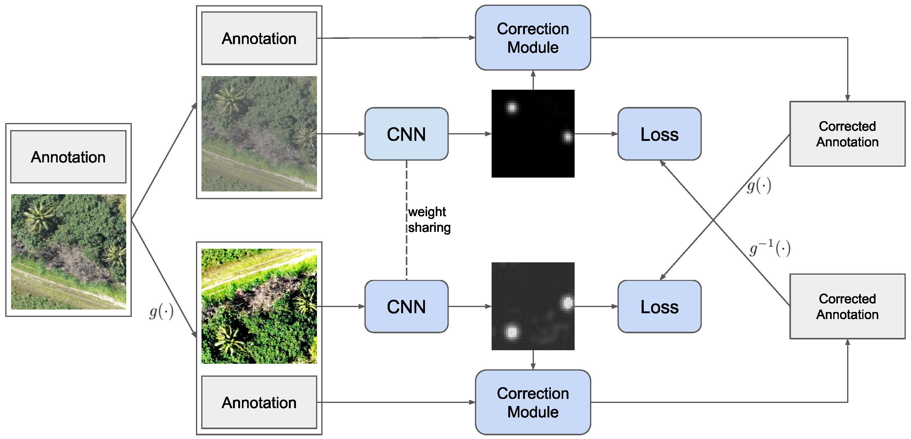
As depicted in the overview in Figure 1, we first created two transformed versions and of I by image augmentation with color jitter, image noise, flipping, and transposing. Without loss of generality and to simplify the notation, we assumed that is obtained without geometric transformations and that the coordinate space of the original annotations is aligned with . For , we denoted the geometric transformation with and its inverse with , i.e., is aligned with .

Figure 1.
Our proposed co-correction framework. Two image versions are created and fed through a Siamese network. The outputs are used to generate corrected annotations, which are, in turn, employed as supervision for the other branch. In doing so, we need to apply the geometric transformation to the upper branch and undo it on the lower branch with . Aerial image from [48].
Thereafter, we fed both and into and obtained our class activation maps and . Together with the noisy locations and , these were used by our correction scheme (see next section) to generate improved locations and , respectively. To avoid cascading errors, we always used the original noisy locations for the initialization in the correction algorithm instead of corrected locations from a previous epoch. Furthermore, note that is geometrically aligned with .
Similar to [20,31,32,33,35], we employed the corrected object centers resulting from one branch, i.e., one image version, to supervise the network output of the other branch. Therefore, we dubbed our method co-correction. This technique has the advantage of reducing self-confirmation bias, which can occur if the supervision used to update a network is generated by the same network with the same data.
We utilized a pixelwise target for containing Gaussian kernels around the corrected locations . More precisely, for all , we set
Here, the standard deviation is a predefined hyperparameter and the normalization factor of the bivariate normal density function is omitted to obtain a reasonable scale for the target values. Analogously, the target for arises from .
As the loss function, we chose the binary cross-entropy, which is also suitable for our soft targets. That is,
where
An illustration of the described process that offers more detail than the overview in Figure 1 can be found in Figure 2.
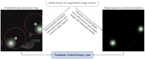
Figure 2.
Detailed illustration of the proposed correction mechanism to learn class activation maps. Red and green crosses indicate noisy and corrected object locations, respectively. Dashed, red circles around red crosses show which pixels impact the correction of the respective object location. After applying Algorithm 1, corrected locations are exchanged with the partner branch and pixelwise targets are created to ultimately compute a pixelwise loss. Best viewed in color.
The reasons for using soft targets instead of deterministic target distributions for the pixels are twofold: first, the softness reflects the uncertainty in the target distribution due to the label noise. Furthermore, second, when given point labels, it is the natural choice to use Gaussian blobs to localize the objects in the target. Using deterministic targets of a certain shape always poses a stronger assumption on the underlying features. If such assumptions can be justified—for instance, because not only point labels but also the spatial extents of the objects are given—it can of course be sensible to adjust the targets accordingly. Let us also note that, this way, soft targets are theoretically possible. However, in practice, this hardly occurs, and is not detrimental for training.
| Algorithm 1: Label Correction |
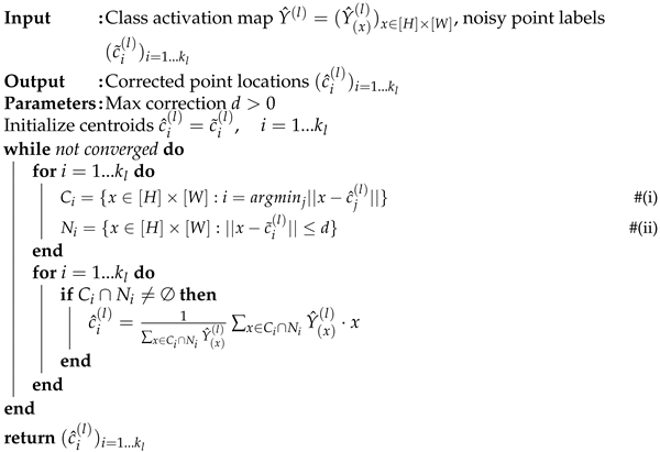 |
4.2. Label Correction
Once we obtained an activation map, we employed Algorithm 1 to refine the original noisy object locations. This algorithm is a modified version of the weighted k-means clustering algorithm, which we applied to pixel locations. More precisely, we initialized the centroids as the given noisy object locations . Then, we iteratively updated the centroids as the weighted mean of pixels that are (i) closer to the respective centroid than to all other centroids and (ii) within a range of d from the original centroid. The weights correspond to the activations from the activation map learned in the previous step.
Apart from restriction (ii), this is exactly the weighted k-means algorithm applied on pixel locations. The underlying idea is that we wanted to place each point label into a local center of (relatively) high activations. Simultaneously, we wanted to avoid placing all point labels in the same location. In addition, we included restriction (ii), which limits the displacements and, therefore, introduces the principle of locality. This reflects the assumption that the noisy labels are still reasonably close to the true locations, and it prevents erroneous and distant activations from distorting the other centroids. In other words, when trying to find the optimal label position for an object in one image corner, we did not have to take distant pixels in opposite corners into account. This robustness, and the property that a slight activation near a noisy label suffices in attracting and correcting the label, are the main advantages of the proposed algorithm.
4.3. Box Size Estimation
On some occasions, it might be necessary to not only estimate the locations, but also the spatial extents of objects. To address this additional problem, we proposed a simple method (see Algorithm 2) that allowed us to estimate the object sizes from the learned class activation maps. The inputs for this method are the predicted class activation maps and the corrected object centers. Furthermore, a standard box size as an initial guess for the object size is required. To choose this hyperparameter, one can use an estimated average object size for a class or employ prior knowledge.
In the algorithm, we determined the set of pixel locations that are assigned to the respective centroid for every object present in the image. From these locations, we disregarded the ones with an activation below a certain threshold . The first estimate for the box shape is then the minimal bounding box around the locations in this cluster of activated pixels. As this estimate is not always reliable, we further refined it in two ways. First, depending on the hyperparameter setup and the class activation maps, this method tends to overestimate the real sizes of objects. Therefore, we introduced an additional hyperparameter , with which, we scale down the estimated box size. Furthermore, second, to counter the effect of false or missing activations, we take a convex combination of the estimated box with the initial, standard-sized box. The proportion parameter for the convex combination is chosen according to the average confidence in the activations for this object. The exact choice of the function to determine has no special justification and may also be seen as a subject to tuning.
| Algorithm 2: Box Size Estimation |
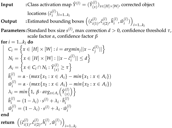 |
4.4. Overall Training Process
When using this method, we trained the network as described in Figure 1. Before we started with the co-correction, we trained on the uncorrected, raw labels for a few epochs in a warm-up phase. The usage of corrected targets during training supports the learning process (see Section 5.5). After determining the corrected object locations with the fully trained network and the proposed label correction method (Algorithm 1), one can use Algorithm 2 to estimate box sizes and shapes if desired. Finally, the refined annotations were stored and used as the ground truth for training object detectors in a second training stage. Note that, for every image, our correction scheme outputs exactly as many object locations as it received as an input. Therefore, our method only deals with bounding box noise and not with noise regarding the object classes. Furthermore, our method is not directly involved in the final training of the object detector. Hence, it is arbitrarily combinable with other object detection methods having certain strengths (see Appendix A). For example, wrong class labels could be corrected with methods such as [18,35] after our correction of locations has been applied.
5. Experiments
5.1. Setting and Data
We evaluated our label correction method on three datasets: COWC [49], NWPU VHR-10 [29], and a third dataset published in [48], which we subsequently refer to as PalmTrees. The datasets contain objects from different domains, such as vegetation, urban artifacts, and means of transport. By this choice, we want to demonstrate that our method is not restricted to a specific use case, but is rather suitable for many different applications in remote sensing. As all of these datasets are annotated with clean labels, we simulate localization noise in our experiments.
5.1.1. COWC
This dataset contains aerial imagery of multiple locations and was published for the task of detecting vehicles. We sliced the images into patches of 512 by 512 pixels and used random splits of 10% for validation and testing, respectively. The original labels are provided as points representing the centers of the cars. For our label correction scheme, we could directly use these point labels, whereas for training object detectors, we created a bounding box with a fixed size around each center. For the size, we chose 32 pixels, corresponding to a height and width of 4.8 m, as the standardized pixel size is 15 cm.
To simulate annotation noise, we displaced the vehicle locations with Gaussian noise with a mean of zero and a standard deviation of 16 pixels. Labels being located outside the image extent after adding the noise were removed. Apart from that, all labels were kept and only their locations were manipulated. Altogether, our simulation of noise results in an average intersection over union (IoU) of roughly 30% when comparing the corrupted with the ground-truth boxes.
5.1.2. PalmTrees
Apparently, the objects of interest in this aerial image dataset are palm trees. Once again, we extracted patches of 512 by 512 pixels. The annotation consists of a set of GPS coordinates, which are also available at OpenStreetMap. In the training of object detectors, we assume a fixed size of 64 pixels for the trees. With a ground sampling distance of 8cm, this corresponds to a tree diameter of 5.12 m. Since the alignment of the point annotations with the imagery has already been corrected in this imagery, we simulate noisy locations by adding Gaussian noise with zero mean and a standard deviation of 24 pixels to the initial positions.
5.1.3. NWPU VHR-10
Compared to the first two datasets, this dataset is more diverse. Instead of a single class, it contains objects of ten different classes: bridge, harbor, airplane, ship, vehicle, storage tank, baseball diamond, tennis court, basketball court, and ground track field. The image sizes vary, which is why we rescaled every image to 1024 by 1024 pixels. Here, the original annotations are also complete bounding boxes instead of just single point locations, as these objects have a larger variation in their sizes. However, for our method, we only used the box centers and the average box sizes per class to create training targets. For the standard deviations of the simulated Gaussian localization noise, we used one third of the average box size in pixels for each class. As this dataset contains precise information on the object sizes, we used it to evaluate our box size estimation method. For the other two datasets, this part of our framework was omitted because we could not evaluate it with the given annotations.
5.2. Implementation and Training Details
5.2.1. Co-Correction
For our label correction technique, we used a pretrained ResNet-50 [50] with a reduced stride in the last two layers; that is, the resolution of our class activation maps is one eighth of the input. Furthermore, we applied the sigmoid function to the outputs to ensure that the activations lie within . The Gaussian blobs for the targets were created with standard deviations depending on the dataset and the object class. We noticed that reducing the width of the target blobs, compared to the standard deviations of the noise, led to better results due to a better separation of single instances. Moreover, we augmented the training images by mirroring, adding noise, and color jittering. As an optimization algorithm, we used Adam [51].
Before feeding the obtained class activation maps into our label refinement algorithms (Algorithms 1 and 2), we preprocessed them by setting small values (below 0.01) to zero and taking the fourth power to obtain a better distinction of activated and non-activated regions. Discarding the small activations is especially essential for the box estimation, which is why we explicitly included this in Algorithm 2.
5.2.2. Object Detection
In our experiments, we demonstrated the effectiveness of our method by comparing the performance of different (noise-robust) object detection frameworks when trained on noisy, corrected, and clean labels, respectively. In particular, we used RetinaNet [52] and Faster R-CNN [53], as well as Noise-resistant Faster R-CNN [18], Faster R-CNN trained with the annotation refinement of [36], and RetinaNet trained with co-teaching [35].
As the code for the latter three training strategies is not (yet) published, we implemented them ourselves. For this, we stuck as close as possible to the descriptions in the papers and plugged the modifications into the Faster R-CNN or RetinaNet architecture, respectively. In particular, for co-teaching, we used RetinaNet as a one-stage detector and, for the Noise-resistant Faster R-CNN and annotation refinement, we employed the Faster R-CNN architecture. Moreover, we omitted the soft label correction module in the Noise-resistant Faster R-CNN, as it is not necessary in our setting without label noise. To achieve a fair comparison, all detectors were equipped with a pretrained ResNet-50 backbone. Approaches based on RetinaNet were trained with Adam, whereas the Faster R-CNN architectures achieved a better performance with SGD and a momentum of 0.9.
We used Hyperopt [54] for the hyperparameter search in all experiments. Details on the best hyperparameter settings can be found in Appendix B. Furthermore, our experiments were executed on a single NVIDIA GeForce RTX 2080 Ti or a comparable device.
5.3. Quantitative Results and State-of-the-Art Comparison
The most straightforward way to evaluate our correction method is to directly measure the distances between the corrected locations and their ground-truth locations. The effectiveness of our approach is demonstrated by the decrease in root-mean-square errors (RMSE) between the refined labels and their ground-truth counterparts in Table 1. As a baseline, we used the noisy object locations without any preprocessing. The corrected labels were obtained by our method when training only with the initial noisy annotations. Even if the improvement is substantial, the corrected labels still do not perfectly match their true positions. Nonetheless, this improvement is crucial for the training of object detectors, which we analyze in the following.

Table 1.
RMSE between the noisy and corrected object locations and their closest ground-truth object center. For NWPU VHR-10, we normalized the Euclidean errors (in pixels) with the average box size for each class to prevent classes of larger objects from dominating the class macro average of RMSEs.
We trained object detectors with different approaches and settings and, thereafter, conducted a thorough comparison (see Table 2). As a measure for performance, we chose the widely used mean average precision (mAP) with an IoU threshold of 0.5 on the test set. In the first two sections of the table, only noisy annotations containing square boxes of a fixed size for each class (we consider this as equally informative as point labels) were used for training the models. In the second section, we applied our refinement method on the noisy annotations before training the detectors. For NWPU VHR-10, we also employed our box size estimation. Since none of the existing methods are designed to estimate box sizes from scratch, i.e., without even noisy boxes sizes as supervision, a direct comparison of these methods with our framework is not valid when integrating the box size estimation. Nevertheless, we included the scores for the sake of completeness and to show the practical use of this technique. The box size estimation setting was omitted for the other two datasets, as their point label annotations do not allow for a meaningful evaluation. We also included the scores for RetinaNet and Faster R-CNN when training with the clean and complete ground-truth bounding box annotations to obtain an upper bound for the performance on noisy labels.
Table 2.
mAP scores (in percent) for different object detection methods and datasets at test time. Results in the first, second, and third section were obtained when training on noisy, our refined, and clean ground-truth annotations, respectively. Scores for ground-truth labels serve as an upper bound for the models in the first two sections.
From the existing methods, the annotation refinement of [36] and especially the Noise-resistant Faster R-CNN of [18] are the best-performing. Unfortunately, we were not able to reproduce the promising results of the co-teaching approach of [35]. However, it is evident that our label, co-correction, is superior to all other methods for dealing with localization noise. For COWC and PalmTrees, it largely closes the gap between noisy and clean supervision. On NWPU VHR-10, this gap remains rather large, which we found out to be primarily caused by inaccurate box sizes, and not their locations. Note that our setting for NWPU VHR-10 poses noisy and weak supervision, making it more challenging.
We reason that the main advantage of our approach is that it makes maximal use of every single label. Our correction scheme is forced to move every label to a position that is in agreement with the learned features. At this position, rather low activations in the true position suffice to correct the label if the surrounding activations are even lower. Another advantageous feature of our label correction is that the locations are optimized jointly and not independently from each other, i.e., the correction of one label influences the correction of other nearby labels. Our method fulfills this property because it is based on k-means clustering. Thus, the cluster centroids, i.e., the corrected labels, cannot degenerate and share the same location. This property is especially useful when objects are close to each other and, for example, the noise shifts a label to a neighboring object. In such a scenario, our method will mostly avoid assigning two labels to one object while assigning no label to the other object. In the COWC dataset, this kind of situation can particularly occur in parking areas, where many vehicles are densely located in a small region.
5.4. Ablation Study
Since it is the only dataset where our full framework was employed, we conducted an ablation study on the NWPU VHR-10 dataset. The scores measuring the quality of the corrected and refined labels are given in Table 3. The “Initial noisy annotations” are the boxes with a fixed size per class and a randomly displaced center. The “Refined locations (single branch)” were obtained with our proposed correction framework but with only a single branch, i.e., the supervision for an output was generated based on the very same output. As we can see from the large margin in the scores, our correction method is highly effective. If we add a second branch (“Refined locations (co-correction)”), the score is improved once again. However, the gap is rather marginal and, in cases where the computational overhead caused by the second branch is an issue, the single-branch method might be preferable. This method does not make any improvements on the box sizes and shapes and, therefore, we can achieve another substantial increase for the score if we employ our box size estimation (“Full (co-correction + box size estimation)”). The effect of the box size estimation can also be observed in Table 2. However, the weakest point of our overall framework is the estimation of box sizes. We noticed that, in some cases, the class activation maps adopt the shapes of the Gaussian kernels in the targets instead of directly relating the activations to the present objects and their spatial extents. This can hurt the quality of the estimated box sizes, but it has barely any impact on the object localization.
Table 3.
Ablation study on NWPU VHR-10 with scores for the quality of annotations obtained in different settings. The scores are the percentages of boxes having an IoU of at least 0.5 with their corresponding ground truth box.
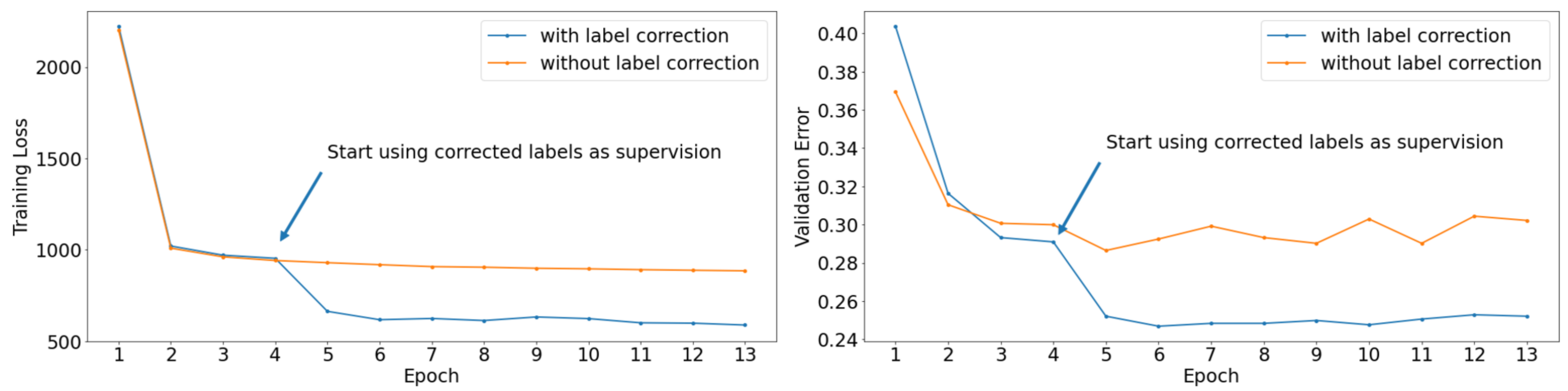
To provide further insights, we compare training and validation curves for training with and without co-corrected supervision on the PalmTrees dataset in Figure 3. The validation errors are the percentages of corrected labels that are not located in a square box around their corresponding ground-truth label. The size of these boxes was chosen to be 32 pixels, which is half the height and width of the ground-truth boxes we used for evaluating the object detectors on this dataset. When we start applying our co-correction scheme and use the corrected labels as supervision, both the training and the validation errors drop instantly. At the same time, if the corrected labels are not used for supervision, the losses and validation errors stay at a relatively high level. Hence, using our corrected labels as supervision is extremely beneficial for the learning process, as not only does it decrease the training loss, but it also improves the performance on unseen data.
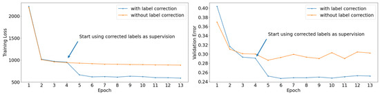
Figure 3.
Training loss (left) and validation error (right) when training with and without co-corrected labels on the PalmTrees dataset. Best viewed in color.
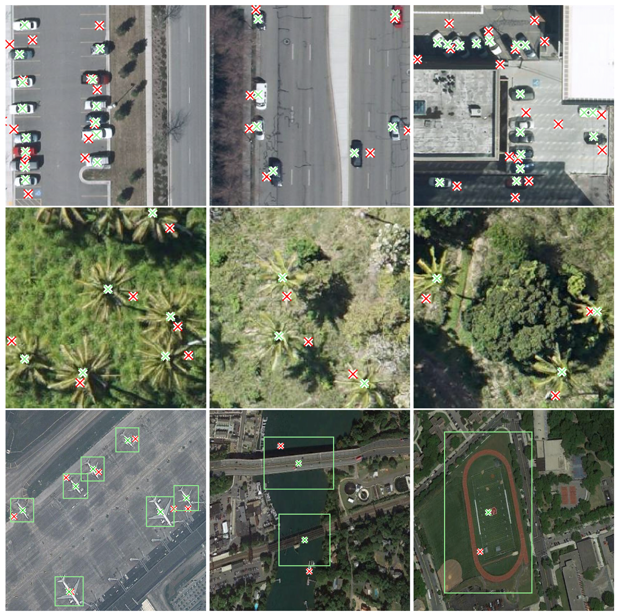
Figure 4 depicts some qualitative examples of how our correction method behaves in practice. As can be seen, it leads to a much better object localization, which, in turn, allows for a much better training of object detectors. Furthermore, the predicted box shapes are decent estimates for the real object extents. The only failure case among these examples can be observed in the top right. Here, one label is placed in the middle of two neighboring cars, whereas another car is covered by two labels. However, in this case, a manual assignment of labels to objects is not straightforward here, as the displacements due to the noise are occasionally larger than the distances between objects. Furthermore, it is noteworthy that, even under the hard conditions in this example, no label is placed into a region of no object by our correction mechanism.
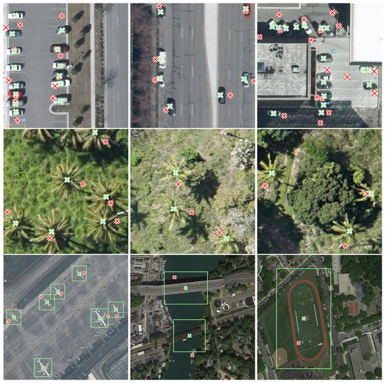
Figure 4.
Corrected labels for examples of the COWC (first row), PalmTrees (second row), and NWPU VHR-10 (third row) dataset. Original noisy and refined labels are marked with red and green crosses, respectively. For the NWPU VHR-10 dataset, we additionally depict our estimated bounding boxes. Best viewed in color.
In addition, we also show some learned class activation maps in Figure 5. Again, our correction method still works in crowded scenes with many objects, and the separation of single instances is consistently good. Furthermore, we can see that the class activation maps provide meaningful information on the spatial extents of the objects. We utilize this in our bounding box size estimation. However, in some cases, and particularly for some classes, such as the baseball field on the right, the class activation maps adopt the Gaussian kernel shapes from the training targets, making it harder to estimate object sizes from them. We can definitely see potential for improvement with respect to that in the future. Nevertheless, this behavior does not harm the correction of object locations, which works well on all datasets and classes we used for our experiments.
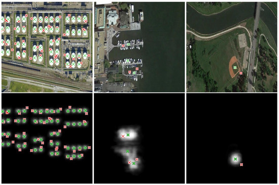
Figure 5.
Example images, class activation maps, and object labels from the NWPU VHR-10 dataset. Noisy and refined labels are marked with red and green crosses, respectively. Best viewed in color.
5.5. Qualitative Results
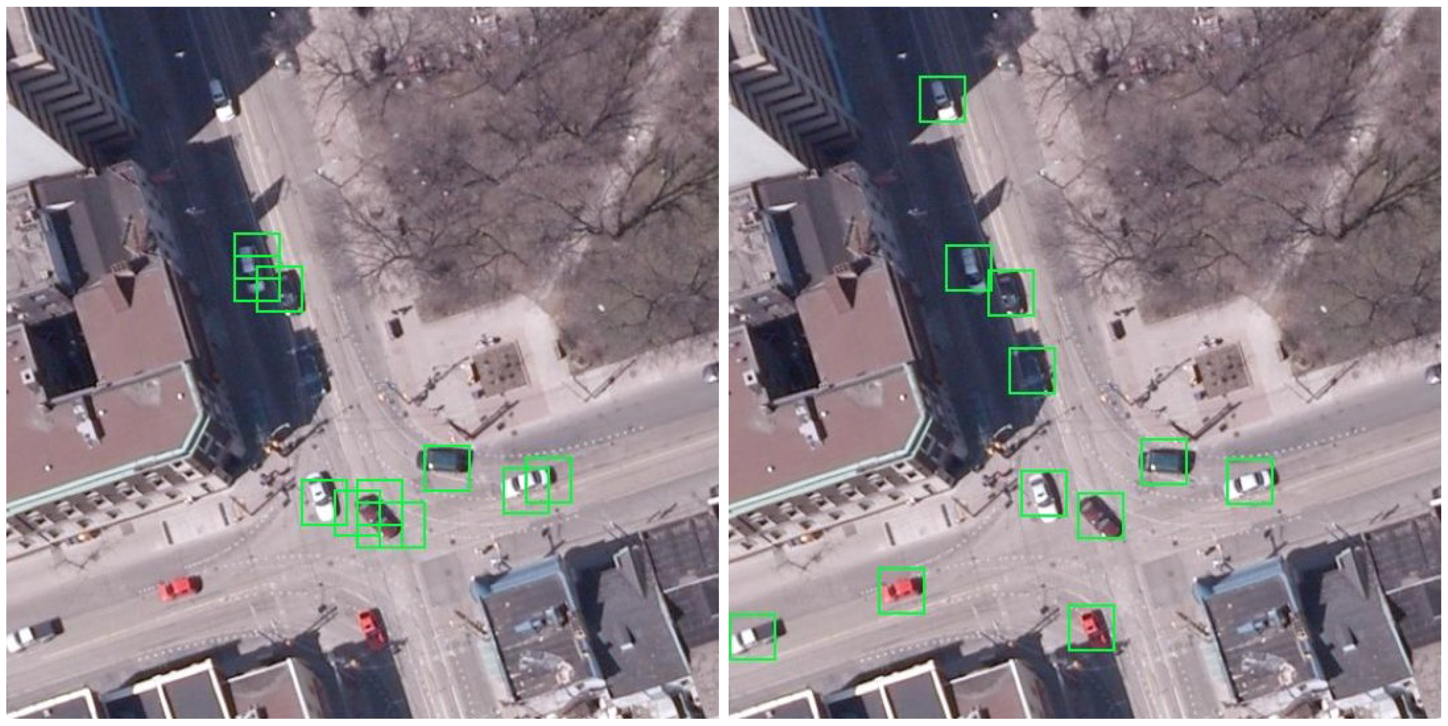
As a third visual example, we depict the predictions of a RetinaNet trained with and without corrected labels in Figure 6. The predictions on the left were obtained after training on the original noisy annotations and the predictions on the right were obtained after training with our corrected object locations. We can see that poorly placed anchors have a relatively high confidence, which leads to imprecise and redundant predictions. This is caused by noisy labels providing positive supervision for these anchors during training. Consequently, the network struggles to learn a distinction between well-placed and poorly placed bounding boxes. This effect does not occur with our corrected annotations, demonstrating the benefit of our method.
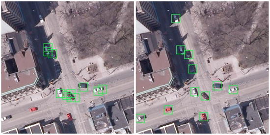
Figure 6.
Predictions of RetinaNet on COWC when trained on noisy annotations (left) and corrected annotations (right). Best viewed in color.
6. Conclusions
In this work, we propose a label correction technique that can be employed for training object detectors with annotations only containing noisy object locations as points. It consists of a co-correction training framework to learn class activation maps and object locations in a noise-robust way. Moreover, the correction module works in a one-to-one manner, i.e., it proposes exactly one corrected location for every noisy point label. On top of that, we used our learned class activation maps to estimate bounding box sizes, making our framework applicable in settings with noisy and weak supervision.
A major advantage of our method is that it can be seen as a label preprocessing step, which makes it able to be combined with any other approach for (noise-tolerant) object detection. In doing so, we observed a remarkable improvement in performance when training on our corrected labels instead of the initial noisy annotations. The most room for improvement of our framework lies in the estimation of precise bounding boxes. Our approach is rather simple and is mainly conceived to demonstrate an additional use of our learned class activation maps. However, more sophisticated machinery may produce better box estimates. Furthermore, it will be interesting to integrate our technique into an end-to-end trainable approach and also to extend it to deal with other types of annotation noise in the future. Particularly, sparsely annotated datasets, i.e., datasets where annotations are missing for an unknown subset of objects [1,20], pose a problem that is not addressed by our study.
In the context of remote sensing, we hope that this work is a first step toward the successful usage of GPS annotations for object detection. This would improve the practicability of these powerful methods in many real-world applications. For instance, in vegetation monitoring, GPS records resulting from field surveys could be employed to train object detectors on corresponding aerial imagery. Subsequently, expensive field surveys may be replaced by cheaper aerial surveys. Another use case could be urban planning, where existing data from GIS, e.g., building locations, may be aligned with aerial or satellite images more precisely.
Author Contributions
Conceptualization, M.B. and M.S.; methodology, M.B. and M.S.; software, M.B.; validation, M.B.; formal analysis, M.B.; investigation, M.B.; resources, M.S.; data curation, M.B.; writing—original draft preparation, M.B.; writing—review and editing, M.B. and M.S.; visualization, M.B.; supervision, M.S.; project administration, M.S.; funding acquisition, M.S. All authors have read and agreed to the published version of the manuscript.
Funding
This work has been funded by the German Federal Ministry of Education and Research (BMBF) under Grant No. 01IS18036A. The authors of this work take full responsibilities for its content.
Institutional Review Board Statement
Not applicable.
Informed Consent Statement
Not applicable.
Data Availability Statement
At the time of writing, all datasets used in this study are publicly available. The COWC datset [49] can be downloaded here https://gdo152.llnl.gov/cowc/ (accessed on 5 October 2021), the NWPU VHR-10 dataset [29] here https://drive.google.com/open?id=1--foZ3dV5OCsqXQXT84UeKtrAqc5CkAE (accessed on 5 October 2021), and the data for the palm tree detection challenge [48] here https://docs.google.com/document/d/16kKik2clGutKejU8uqZevNY6JALf4aVk2ELxLeR-msQ/edit (accessed on 5 October 2021).
Conflicts of Interest
The authors declare no conflict of interest.
Appendix A. Combination with Other Methods
In Table A1, we evaluate different object detection methods on different sets of labels on the COWC dataset. This also includes the combinations of our approach with other noise-robust methods. The effectiveness of our proposed label correction technique can be seen in the rightmost column with the scores for the detectors trained on corrected labels. These values show that the improvement due to our label correction is much more influential than the improvements due to the noise-tolerant training methods of existing works.
From the existing methods, the annotation refinement [36] and the Noise-resistant Faster R-CNN [18] outperform the others regarding the noisy setting. They also lead to an improvement over the vanilla Faster R-CNN with corrected labels, which indicates that our method can indeed be combined with other techniques. However, when training on corrected labels, the vanilla RetinaNet seems to outperform all of the noise-tolerant models. As we already mentioned in the paper, we were not able to produce good results with co-teaching for object detection [35]. Often, the best scores for this method were observed during the warm-up phase and, during the actual training with a selected set of annotations, the performance decreased. This effect might occur because, in our setting, each annotation provides at least a rough localization of the object and is thus still informative. Supervision with these rough locations could therefore be better than ignoring these “hard” instances completely.
Appendix B. Hyperparameters
Here, we give details on the best hyperparameter configurations for different models and datasets. In general, we used an Adam optimizer for RetinaNet-based methods and SGD with a momentum of 0.9 for Faster R-CNN-based methods. Furthermore, the ReduceOnPlateau learn rate scheduler of Pytorch was used in all experiments, with a decay rate of 0.1. As already mentioned in the paper, we employed Hyperopt [54] for searching the best hyperparameters. Depending on the number of hyperparameters and their possible range, we conducted the searches with different numbers of runs. From these runs, we chose the one with the best performance on the validation set for every method and reported its performance on the test set.
Table A1.
Average precision scores (in percent) on the COWC dataset when training on different sets of labels. †, Faster R-CNN architecture; ‡, RetinaNet architecture.
Table A1.
Average precision scores (in percent) on the COWC dataset when training on different sets of labels. †, Faster R-CNN architecture; ‡, RetinaNet architecture.
| Method | Noisy | Corrected |
|---|---|---|
| Faster R-CNN † | 39.9 | 78.8 |
| RetinaNet ‡ | 39.5 | 85.0 |
| Co-teaching ‡ | 38.3 | 81.9 |
| Noise-resistant Faster R-CNN † | 54.4 | 83.5 |
| Annotation Refinement † | 44.1 | 83.2 |
Appendix B.1. Co-Correction
In Table A2(a), we list the hyperparameter settings for our co-correction method. Here, refers to the standard deviation of the Gaussian kernels in the targets. Apparently, choosing this standard deviation to be significantly smaller than the average object sizes is advantageous. We reason that this allows for a better separation of single instances. Note that denotes the average box size for class l on NWPU VHR-10. Parameter d refers to the maximum correction distance in Algorithm 1 in the paper.
Appendix B.2. Label Correction and Box Size Estimation
For the correction of object locations (Alogorithm 1 in the paper), the only hyperparameter is the maximum correction distance d. This was chosen to be 64 for COWC and PalmTrees and for NWPU VHR-10.
Table A2(b) contains the best hyperparameters for our box size estimation on the NWPU VHR-10 dataset. The parameter names correspond to the names in Algorithm 2 in the paper. Once again, the standard box size was chosen as the average box size per class.
Table A2.
Best hyperparameters for our label refinement techniques: (a) co-correction; (b) box size estimation (Algorithm 2).
Table A2.
Best hyperparameters for our label refinement techniques: (a) co-correction; (b) box size estimation (Algorithm 2).
| (a) | |||
| Parameter | COWC | Palm Trees | NWPU VHR-10 |
| Learn rate | 5 × 10⁻⁴ | 5 × 10⁻⁵ | 5 × 10⁻⁵ |
| Batch size | 8 | 8 | 1 |
| Best epoch | 5 | 5 | 35 |
| Warm-up epochs | 2 | 2 | 32 |
| 6.5 | 12.0 | ||
| d | 64 | 64 | |
| (b) | |||
| Parameter | NWPU VHR-10 | ||
| d | 64 | ||
| 0.01 | |||
| 0.8 | |||
| 2 | |||
Appendix B.3. RetinaNet and Faster R-CNN
The best hyperparameter configurations for the standard object detectors RetinaNet [52] and Faster R-CNN [53] are given in Table A3(a,b). The four sections correspond to the different label sets and noise settings. The “Estimated Boxes” section refers to the annotations obtained with our correction of locations and our estimation of box sizes. On COWC and Palm Trees, we did not apply our box estimation scheme, as the available point labels do not allow us to sensibly evaluate it (all objects are assumed to be of the same size).
Appendix B.4. Co-Teaching
Our hyperparameters for the co-teaching approach for object detection [35] are listed in Table A3(c). The q-step parameter denotes the amount by which we increase q with every epoch after the warm-up phase. Moreover, q itself is the proportion of highest loss instances omitted for network updating, and is zero during the warm-up phase. Unfortunately, on COWC and NWPU VHR-10, the best performance was achieved during the warm-up phase. That is, the co-teaching method did not actually benefit the training on these datasets.
Appendix B.5. Annotation Refinement
The best results for the method of [36] were observed with the settings given in Table A3(d). The IoU threshold parameter is used to decide when the overlap of a predicted box with a target box is large enough to correct the target box toward the predicted box. The confidence threshold specifies which predictions are confident enough to be the basis for an annotation correction. With -step, we denote the increase per epoch for , where is the weight of the predicted box when taking the convex combination of a predicted and a target box for correction.
Appendix B.6. Noise-Resistant Faster R-CNN
Table A3(e) contains the best hyperparameters for the Noise-resistant Faster R-CNN [18]. The parameter is the step size for the class-agnostic bounding box correction. The background threshold is the value above which we assign instances to the background class. The step size for the class-specific bounding box refinement is denoted with . Surprisingly, much larger values than the reported for (see [18]) led to better results in our experiments.
Table A3.
Best hyperparameter settings for (noise-resistant) object detection methods: (a) RetinaNet; (b) Faster R-CNN; (c) co-teaching; (d) annotation refinement (e) Noise-resistant Faster R-CNN.
Table A3.
Best hyperparameter settings for (noise-resistant) object detection methods: (a) RetinaNet; (b) Faster R-CNN; (c) co-teaching; (d) annotation refinement (e) Noise-resistant Faster R-CNN.
| (a) | |||
| Parameter | COWC | Palm Trees | NWPU VHR-10 |
| Noisy Labels: | |||
| Learn rate | 1 × 10⁻⁴ | 5 × 10⁻⁴ | 5 × 10⁻⁵ |
| Batch size | 4 | 2 | 4 |
| Best epoch | 2 | 35 | 21 |
| Corrected Locations: | |||
| Learn rate | 1 × 10⁻⁴ | 1 × 10⁻⁴ | 5 × 10⁻⁵ |
| Batch size | 4 | 8 | 2 |
| Best epoch | 17 | 65 | 19 |
| Estimated Boxes: | |||
| Learn rate | - | - | 1 × 10⁻⁴ |
| Batch size | - | - | 4 |
| Best epoch | - | - | 17 |
| Clean Labels: | |||
| Learn rate | 1 × 10⁻⁴ | 5 × 10⁻⁵ | 5 × 10⁻⁵ |
| Batch size | 4 | 4 | 2 |
| Best epoch | 13 | 21 | 39 |
| (b) | |||
| Parameter | COWC | Palm Trees | NWPU VHR-10 |
| Noisy Labels: | |||
| Learn rate | 1 × 10⁻³ | 5 × 10⁻⁴ | 1 × 10⁻³ |
| Batch size | 4 | 8 | 2 |
| Best epoch | 6 | 8 | 25 |
| Corrected Locations: | |||
| Learn rate | 5 × 10⁻³ | 5 × 10⁻⁴ | 5 × 10⁻³ |
| Batch size | 4 | 8 | 2 |
| Best epoch | 9 | 6 | 17 |
| Estimated Boxes: | |||
| Learn rate | - | - | 5 × 10⁻³ |
| Batch size | - | - | 2 |
| Best epoch | - | - | 17 |
| Clean Labels: | |||
| Learn rate | 2 × 10⁻³ | 5 × 10⁻³ | 5 × 10⁻⁴ |
| Batch size | 4 | 8 | 1 |
| Best epoch | 12 | 31 | 53 |
| (c) | |||
| Parameter | COWC | Palm Trees | NWPU VHR-10 |
| Learn rate | 1 × 10⁻⁴ | 1 × 10⁻⁴ | 1 × 10⁻⁵ |
| Batch size | 4 | 4 | 1 |
| Best epoch | 3 | 4 | 15 |
| Warm-up epochs | 3 | 1 | 16 |
| q-step | 0.01 | 0.005 | 0.001 |
| (d) | |||
| Parameter | COWC | Palm Trees | NWPU VHR-10 |
| Learn rate | 5 × 10⁻³ | 2 × 10⁻³ | 5 × 10⁻⁴ |
| Batch size | 4 | 4 | 1 |
| Best epoch | 4 | 13 | 45 |
| Warm-up epochs | 3 | 3 | 4 |
| IoU thresh. | 0.5 | 0.25 | 0.25 |
| Confidence thresh. | 0.5 | 0.5 | 0.5 |
| -step | 0.1 | 0.1 | 0.01 |
| (e) | |||
| Parameter | COWC | Palm Trees | NWPU VHR-10 |
| Learn rate | 5 × 10⁻³ | 1 × 10⁻³ | 1 × 10⁻³ |
| Batch size | 8 | 8 | 1 |
| Best epoch | 6 | 9 | 20 |
| Warm-up epochs | 3 | 3 | 8 |
| 800 | 800 | 600 | |
| 0.1 | 0.2 | 0.1 | |
| Background thresh. | 0.99 | 0.99 | 0.99 |
| 0.5 | 0.5 | 0.5 | |
References
- Wegner, J.D.; Branson, S.; Hall, D.; Schindler, K.; Perona, P. Cataloging public objects using aerial and street-level images-urban trees. In Proceedings of the IEEE Conference on Computer Vision and Pattern Recognition, Las Vegas, NV, USA, 27–30 June 2016; pp. 6014–6023. [Google Scholar]
- Fromm, M.; Schubert, M.; Castilla, G.; Linke, J.; McDermid, G. Automated Detection of Conifer Seedlings in Drone Imagery Using Convolutional Neural Networks. Remote. Sens. 2019, 11, 2585. [Google Scholar] [CrossRef] [Green Version]
- Liu, Y.; Cen, C.; Che, Y.; Ke, R.; Ma, Y.; Ma, Y. Detection of Maize Tassels from UAV RGB Imagery with Faster R-CNN. Remote Sens. 2020, 12, 338. [Google Scholar] [CrossRef] [Green Version]
- Veeranampalayam Sivakumar, A.N.; Li, J.; Scott, S.; Psota, E.; Jhala, A.J.; Luck, J.D.; Shi, Y. Comparison of Object Detection and Patch-Based Classification Deep Learning Models on Mid- to Late-Season Weed Detection in UAV Imagery. Remote Sens. 2020, 12, 2136. [Google Scholar] [CrossRef]
- Sirko, W.; Kashubin, S.; Ritter, M.; Annkah, A.; Bouchareb, Y.S.E.; Dauphin, Y.N.; Keysers, D.; Neumann, M.; Cissé, M.; Quinn, J. Continental-Scale Building Detection from High Resolution Satellite Imagery. arXiv 2021, arXiv:2107.12283. [Google Scholar]
- Bai, T.; Pang, Y.; Wang, J.; Han, K.; Luo, J.; Wang, H.; Lin, J.; Wu, J.; Zhang, H. An Optimized Faster R-CNN Method Based on DRNet and RoI Align for Building Detection in Remote Sensing Images. Remote Sens. 2020, 12, 762. [Google Scholar] [CrossRef] [Green Version]
- Rabbi, J.; Ray, N.; Schubert, M.; Chowdhury, S.; Chao, D. Small-Object Detection in Remote Sensing Images with End-to-End Edge-Enhanced GAN and Object Detector Network. Remote. Sens. 2020, 12, 1432. [Google Scholar] [CrossRef]
- Yan, D.; Li, G.; Li, X.; Zhang, H.; Lei, H.; Lu, K.; Cheng, M.; Zhu, F. An Improved Faster R-CNN Method to Detect Tailings Ponds from High-Resolution Remote Sensing Images. Remote Sens. 2021, 13, 2052. [Google Scholar] [CrossRef]
- Shin, S.J.; Kim, S.; Kim, Y.; Kim, S. Hierarchical Multi-Label Object Detection Framework for Remote Sensing Images. Remote Sens. 2020, 12, 2734. [Google Scholar] [CrossRef]
- Yang, X.; Sun, H.; Fu, K.; Yang, J.; Sun, X.; Yan, M.; Guo, Z. Automatic Ship Detection in Remote Sensing Images from Google Earth of Complex Scenes Based on Multiscale Rotation Dense Feature Pyramid Networks. Remote Sens. 2018, 10, 10132. [Google Scholar] [CrossRef] [Green Version]
- Kleebauer, M.; Horst, D.; Reudenbach, C. Semi-Automatic Generation of Training Samples for Detecting Renewable Energy Plants in High-Resolution Aerial Images. Remote. Sens. 2021, 13, 4793. [Google Scholar] [CrossRef]
- Shi, L.; Zhang, F.; Xia, J.; Xie, J.; Zhang, Z.; Du, Z.; Liu, R. Identifying Damaged Buildings in Aerial Images Using the Object Detection Method. Remote Sens. 2021, 13, 4213. [Google Scholar] [CrossRef]
- Wang, Z.; Bai, L.; Song, G.; Zhang, J.; Tao, J.; Mulvenna, M.D.; Bond, R.R.; Chen, L. An Oil Well Dataset Derived from Satellite-Based Remote Sensing. Remote Sens. 2021, 13, 1132. [Google Scholar] [CrossRef]
- Huyan, L.; Bai, Y.; Li, Y.; Jiang, D.; Zhang, Y.; Zhou, Q.; Wei, J.; Liu, J.; Zhang, Y.; Cui, T. A Lightweight Object Detection Framework for Remote Sensing Images. Remote Sens. 2021, 13, 683. [Google Scholar] [CrossRef]
- Ma, H.; Liu, Y.; Ren, Y.; Yu, J. Detection of Collapsed Buildings in Post-Earthquake Remote Sensing Images Based on the Improved YOLOv3. Remote Sens. 2020, 12, 44. [Google Scholar] [CrossRef] [Green Version]
- Li, K.; Wan, G.; Cheng, G.; Meng, L.; Han, J. Object detection in optical remote sensing images: A survey and a new benchmark. ISPRS J. Photogramm. Remote Sens. 2020, 159, 296–307. [Google Scholar] [CrossRef]
- Cheng, G.; Han, J. A Survey on Object Detection in Optical Remote Sensing Images. Isprs J. Photogramm. Remote Sens. 2016, 117, 11–28. [Google Scholar] [CrossRef] [Green Version]
- Li, J.; Xiong, C.; Socher, R.; Hoi, S.C.H. Towards Noise-resistant Object Detection with Noisy Annotations. arXiv 2020, arXiv:2003.01285. [Google Scholar]
- Shao, F.; Chen, L.; Shao, J.; Ji, W.; Xiao, S.; Ye, L.; Zhuang, Y.; Xiao, J. Deep Learning for Weakly-Supervised Object Detection and Object Localization: A Survey. arXiv 2021, arXiv:2105.12694. [Google Scholar]
- Wang, T.; Yang, T.; Cao, J.; Zhang, X. Co-mining: Self-Supervised Learning for Sparsely Annotated Object Detection. arXiv 2020, arXiv:2012.01950. [Google Scholar]
- Zhang, C.; Bengio, S.; Hardt, M.; Recht, B.; Vinyals, O. Understanding deep learning requires rethinking generalization. Commun. ACM 2016, 64, 107–115. [Google Scholar] [CrossRef]
- DiBiase, D.; John, A. The Nature of Geographic Information. An Open Geospatial Textbook. 2008. Available online: https://www.e-education.psu.edu/natureofgeoinfo/node/1672 (accessed on 5 October 2021).
- Hughes, M.L.; McDowell, P.F.; Marcus, W.A. Accuracy assessment of georectified aerial photographs: Implications for measuring lateral channel movement in a GIS. Geomorphology 2006, 74, 1–16. [Google Scholar] [CrossRef]
- Gomez-Candon, D.; López-Granados, F.; Caballero-Novella, J.J.; Peñá-Barragán, J.M.; García-Torres, L. Understanding the errors in input prescription maps based on high spatial resolution remote sensing images. Precis. Agric. 2012, 13, 581–593. [Google Scholar] [CrossRef] [Green Version]
- Río, L.D.; Gracia, F. Error determination in the photogrammetric assessment of shoreline changes. Nat. Hazards 2012, 65, 2385–2397. [Google Scholar] [CrossRef] [Green Version]
- Ozcanli, O.C.; Dong, Y.; Mundy, J.L.; Webb, H.; Hammoud, R.; Victor, T. Automatic Geo-location Correction of Satellite Imagery. In Proceedings of the 2014 IEEE Conference on Computer Vision and Pattern Recognition Workshops, Columbus, OH, USA, 23–28 June 2014; pp. 307–314. [Google Scholar] [CrossRef]
- Hall, A.; Louis, J. Vineclipper: A Proximal Search Algorithm to Tie Gps Field Locations to High Resolution Grapevine Imagery. In Innovations in Remote Sensing and Photogrammetry; Springer: Berlin/Heidelberg, Germany, 2009; pp. 361–372. [Google Scholar] [CrossRef]
- Azim, S.; Rasmussen, J.; Nielsen, J.; Gislum, R.; Laursen, M.; Christensen, S. Manual geo-rectification to improve the spatial accuracy of ortho-mosaics based on images from consumer-grade unmanned aerial vehicles (UAVs). Precis. Agric. 2019, 20, 1199–1210. [Google Scholar] [CrossRef]
- Cheng, G.; Zhou, P.; Han, J. Learning Rotation-Invariant Convolutional Neural Networks for Object Detection in VHR Optical Remote Sensing Images. IEEE Trans. Geosci. Remote. Sens. 2016, 54, 7405–7415. [Google Scholar] [CrossRef]
- Jiang, L.; Zhou, Z.; Leung, T.; Li, L.J.; Fei, L. Mentornet: Learning data-driven curriculum for very deep neural networks on corrupted labels. Int. Conf. Mach. Learn. 2018, 5, 3601–3620. [Google Scholar]
- Han, B.; Yao, Q.; Yu, X.; Niu, G.; Xu, M.; Hu, W.; Tsang, I.; Sugiyama, M. Co-teaching: Robust training of deep neural networks with extremely noisy labels. arXiv 2018, arXiv:1804.06872. [Google Scholar]
- Yu, X.; Han, B.; Yao, J.; Niu, G.; Tsang, I.W.; Sugiyama, M. How does Disagreement Help Generalization against Label Corruption? In Proceedings of the International Conference on Machine Learning, Beach, CA, USA, 9–15 June 2019.
- Li, J.; Socher, R.; Hoi, S.C.H. DivideMix: Learning with Noisy Labels as Semi-supervised Learning. In Proceedings of the 8th International Conference on Learning Representations, ICLR 2020, Addis Ababa, Ethiopia, 26–30 April 2020. [Google Scholar]
- Wei, H.; Feng, L.; Chen, X.; An, B. Combating Noisy Labels by Agreement: A Joint Training Method with Co-Regularization. In Proceedings of the IEEE/CVF Conference on Computer Vision and Pattern Recognition (CVPR), New York, NY, USA, 16–18 June 2020. [Google Scholar]
- Chadwick, S.; Newman, P. Training object detectors with noisy data. In 2019 IEEE Intelligent Vehicles Symposium (IV); IEEE: Piscataway, NJ, USA, 2019; pp. 1319–1325. [Google Scholar]
- Mao, J.; Yu, Q.; Aizawa, K. Noisy Localization Annotation Refinement For Object Detection. In Proceedings of the 2020 IEEE International Conference on Image Processing (ICIP), Beijing, China, 25–28 October 2020; pp. 2006–2010. [Google Scholar] [CrossRef]
- Castells, T.; Weinzaepfel, P.; Revaud, J. SuperLoss: A Generic Loss for Robust Curriculum Learning. In Advances in Neural Information Processing Systems; Larochelle, H., Ranzato, M., Hadsell, R., Balcan, M.F., Lin, H., Eds.; Curran Associates, Inc.: Red Hook, NY, USA, 2020; Volume 33, pp. 4308–4319. [Google Scholar]
- Zhang, X.; Yang, Y.; Feng, J. Learning to localize objects with noisy labeled instances. In Proceedings of the 33rd AAAI Conference on Artificial Intelligence, Honolulu, HI, USA, 27 January–1 February 2019; pp. 9219–9226. [Google Scholar]
- Gao, J.; Wang, J.; Dai, S.; Li, L.J.; Nevatia, R. NOTE-RCNN: Noise tolerant ensemble RCNN for semi-supervised object detection. In Proceedings of the IEEE International Conference on Computer Vision 2019, Seoul, Korea, 27–28 October 2019; pp. 9507–9516. [Google Scholar]
- Chen, T.; Kornblith, S.; Norouzi, M.; Hinton, G.E. A Simple Framework for Contrastive Learning of Visual Representations. In Proceedings of the International Conference on Machine Learning, Long Beach, CA, USA, 13–18 July 2020. [Google Scholar]
- Zbontar, J.; Jing, L.; Misra, I.; LeCun, Y.; Deny, S. Barlow Twins: Self-Supervised Learning via Redundancy Reduction. arXiv 2021, arXiv:2103.03230. [Google Scholar]
- He, K.; Fan, H.; Wu, Y.; Xie, S.; Girshick, R.B. Momentum Contrast for Unsupervised Visual Representation Learning. In Proceedings of the IEEE/CVF Conference on Computer Vision and Pattern Recognition, Silver Spring, MD, USA, 9 September 2020. [Google Scholar]
- Ji, X.; Henriques, J.F.; Vedaldi, A. Invariant Information Distillation for Unsupervised Image Segmentation and Clustering. arXiv 2018, arXiv:1807.06653. [Google Scholar]
- Dijkstra, K.; van de Loosdrecht, J.; Schomaker, L.R.; Wiering, M.A. Centroidnet: A deep neural network for joint object localization and counting. In Joint European Conference on Machine Learning and Knowledge Discovery in Databases; Springer: Berlin/Heidelberg, Germany, 2019; pp. 585–601. [Google Scholar] [CrossRef]
- Ribera, J.; Guera, D.; Chen, Y.; Delp, E.J. Locating Objects Without Bounding Boxes. In Proceedings of the IEEE/CVF Conference on Computer Vision and Pattern Recognition (CVPR), Long Beach, CA, USA, 15–20 June 2019. [Google Scholar]
- Wang, Y.; Hou, J.; Hou, X.; Chau, L.P. A Self-Training Approach for Point-Supervised Object Detection and Counting in Crowds. IEEE Trans. Image Process. 2021, 30, 2876–2887. [Google Scholar] [CrossRef]
- Chen, L.; Yang, T.; Zhang, X.; Zhang, W.; Sun, J. Points as Queries: Weakly Semi-supervised Object Detection by Points. In Proceedings of the IEEE/CVF Conference on Computer Vision and Pattern Recognition, Silver Spring, MD, USA, 9 September 2021. [Google Scholar]
- We Robotics and World Bank. Open AI Challenge: Aerial Imagery of South Pacific Islands. Available online: https://blog.werobotics.org/2018/01/11/open-ai-challenge-2/ (accessed on 30 June 2021).
- Mundhenk, T.N.; Konjevod, G.; Sakla, W.A.; Boakye, K. A Large Contextual Dataset for Classification, Detection and Counting of Cars with Deep Learning. In European Conference on Computer Vision; Springer: Berlin/Heidelberg, Germany, 2016. [Google Scholar]
- He, K.; Zhang, X.; Ren, S.; Sun, J. Deep Residual Learning for Image Recognition. In Proceedings of the IEEE Conference on Computer Vision and Pattern Recognition, Las Vegas, NV, USA, 27–30 June 2016. [Google Scholar]
- Kingma, D.P.; Ba, J. Adam: A Method for Stochastic Optimization. In Proceedings of the 3rd International Conference on Learning Representations, ICLR 2015, San Diego, CA, USA, 7–9 May 2015. [Google Scholar]
- Lin, T.; Goyal, P.; Girshick, R.B.; He, K.; Dollár, P. Focal Loss for Dense Object Detection. In Proceedings of the IEEE International Conference on Computer Vision, Venice, Italy, 22–29 October 2017. [Google Scholar]
- Ren, S.; He, K.; Girshick, R.B.; Sun, J. Faster R-CNN: Towards Real-Time Object Detection with Region Proposal Networks. Adv. Neural Inf. Process. Syst. 2015, 28, 91–99. [Google Scholar] [CrossRef] [PubMed] [Green Version]
- Bergstra, J.; Yamins, D.; Cox, D.D. Making a Science of Model Search: Hyperparameter Optimization in Hundreds of Dimensions for Vision Architectures. In Proceedings of the 30th International Conference on International Conference on Machine Learning, Atlanta, GA, USA, 16–21 June 2013. [Google Scholar]


Publisher’s Note: MDPI stays neutral with regard to jurisdictional claims in published maps and institutional affiliations. |
© 2021 by the authors. Licensee MDPI, Basel, Switzerland. This article is an open access article distributed under the terms and conditions of the Creative Commons Attribution (CC BY) license (https://creativecommons.org/licenses/by/4.0/).