
Gap-Filling Eddy Covariance Latent Heat Flux: Inter-Comparison of Four Machine Learning Model Predictions and Uncertainties in Forest Ecosystem


Abstract
:1. Introduction
2. Materials and Methodology
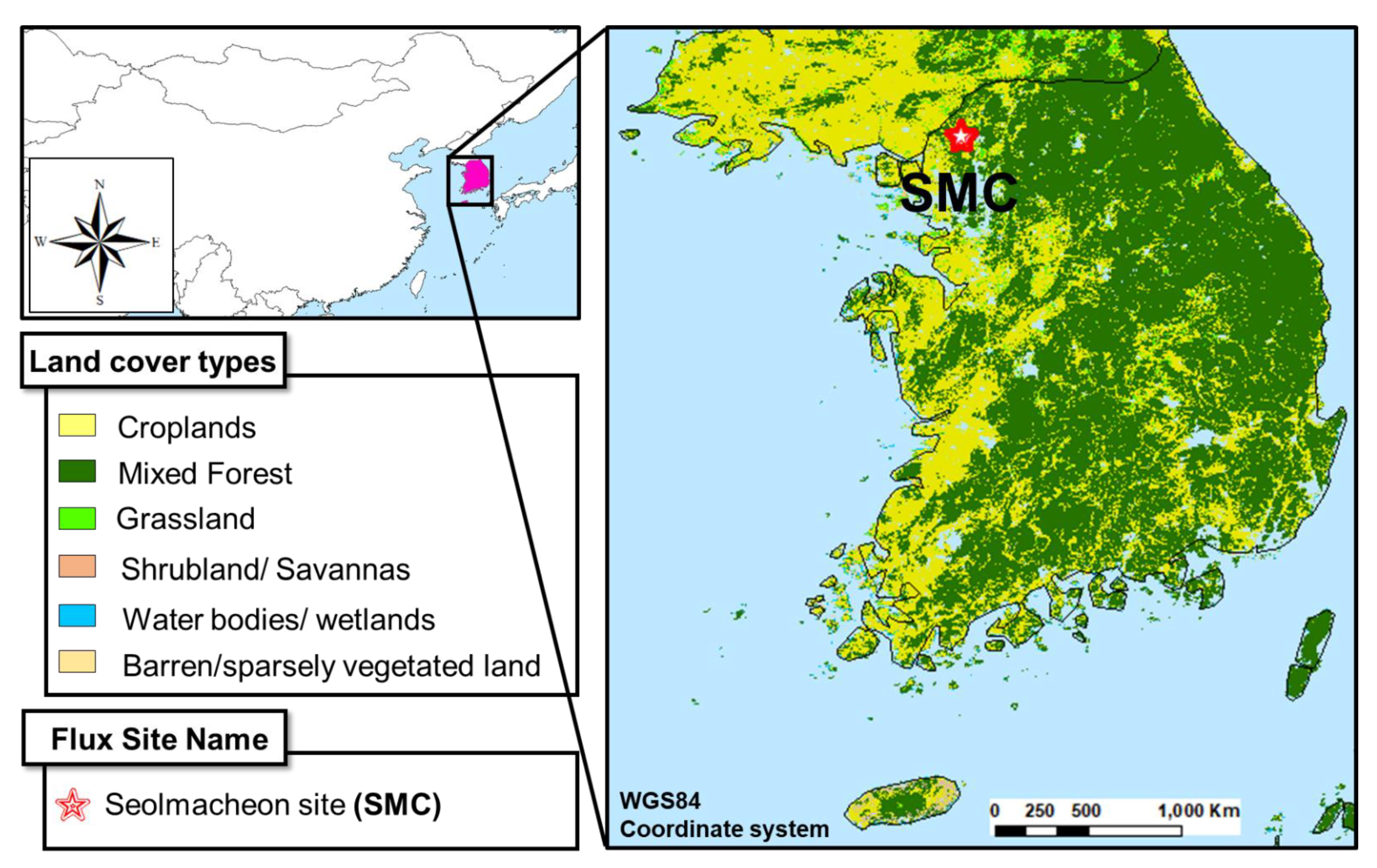
2.1. Study Area and Datasets
2.2. Methodology
2.2.1. ML Models
2.2.2. CNN
2.2.3. SVM
2.2.4. RF
2.2.5. LSTM
2.3. Training of ML Models
3. Performance Metrics
4. Results and Discussion
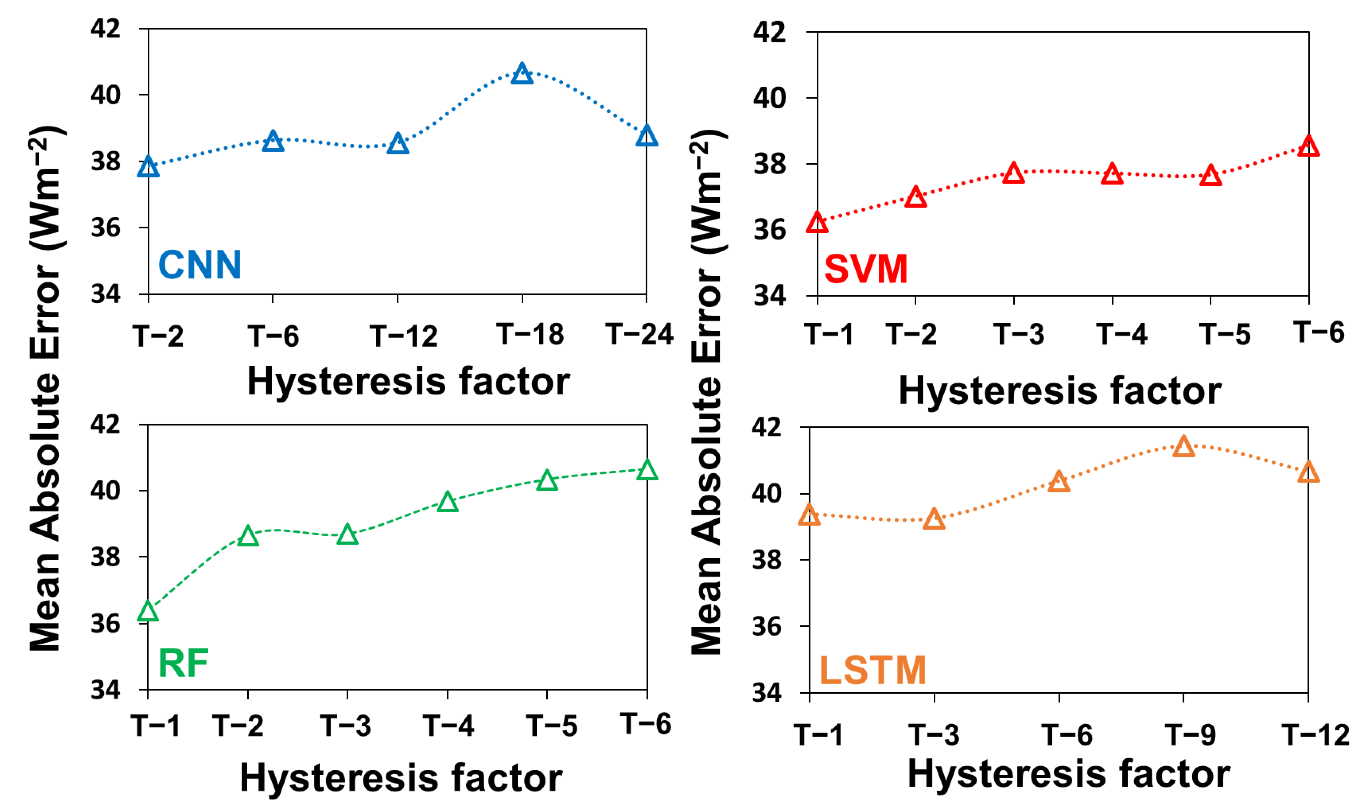
4.1. Optimal Input Combination for Training ML Models
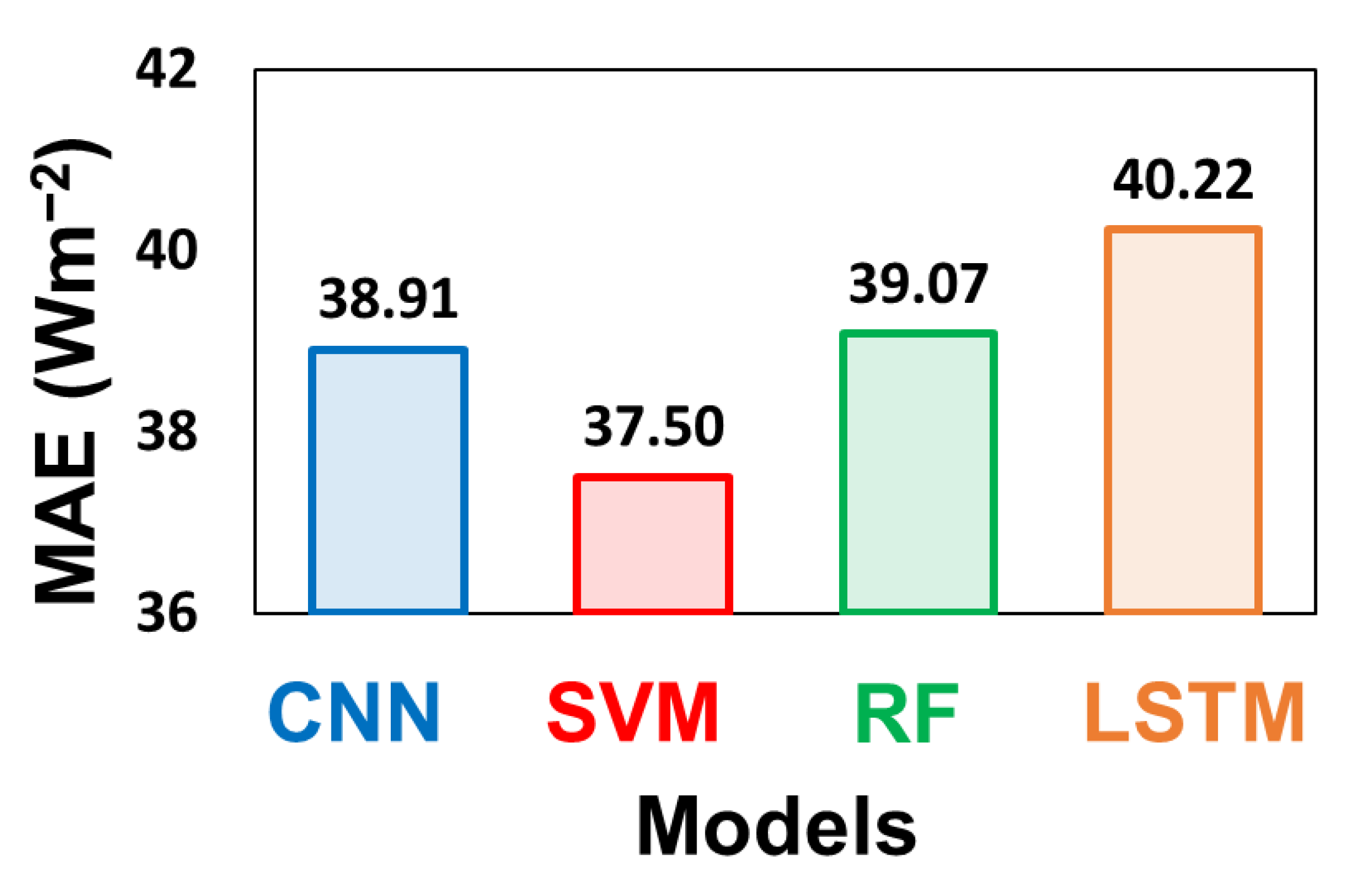
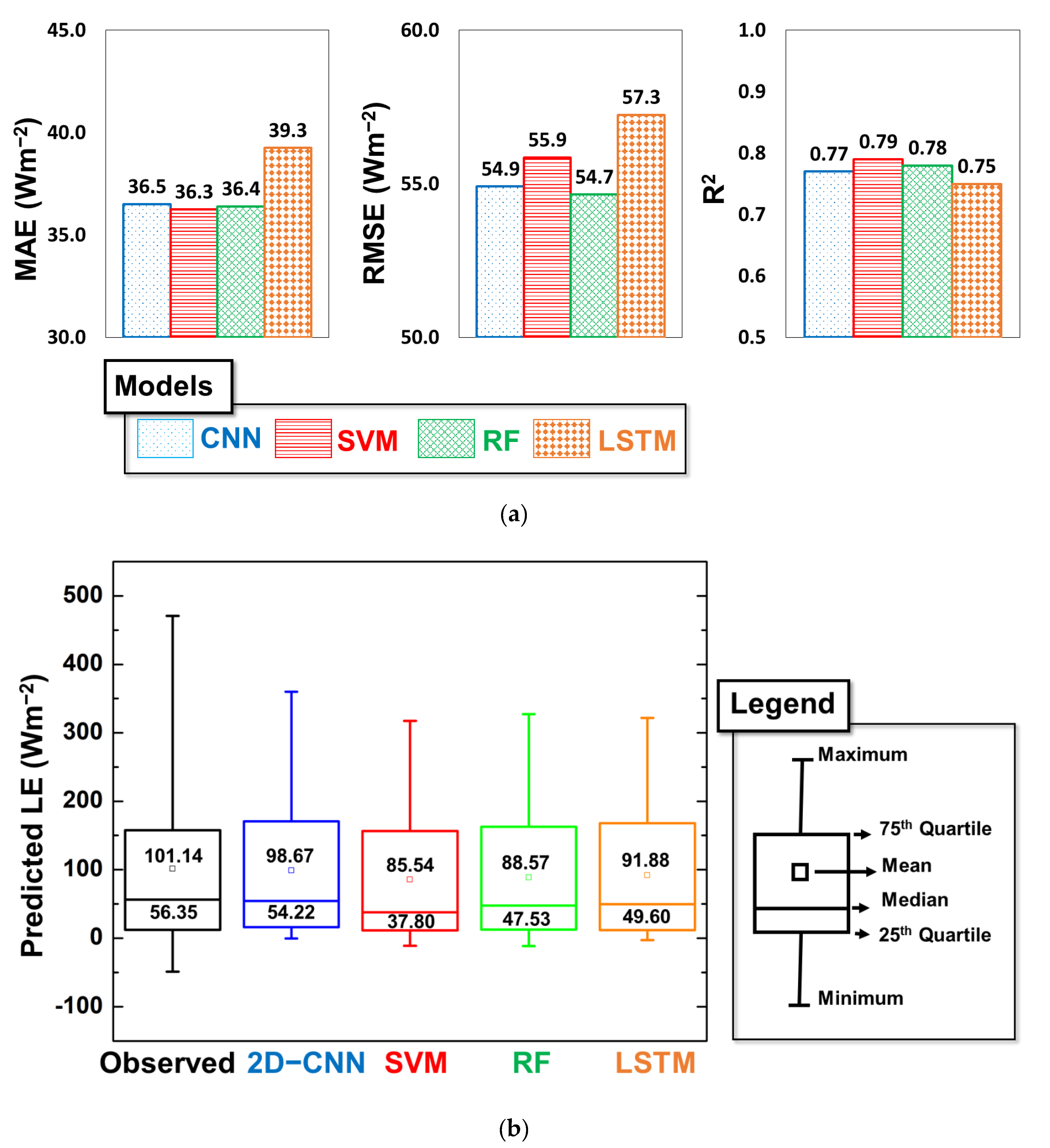
4.2. Statistical Comparison of Gap Filling Based on ML Models
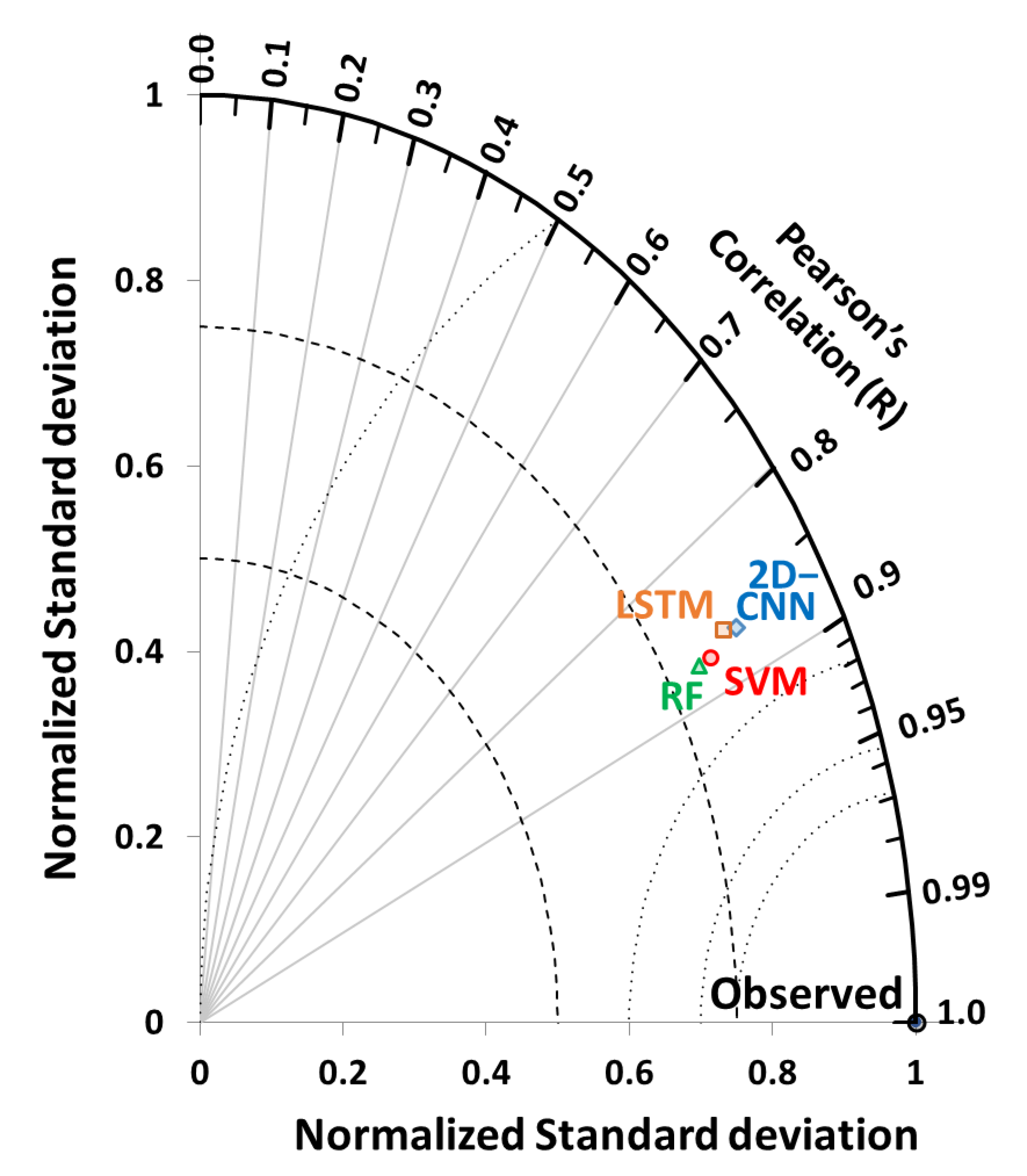
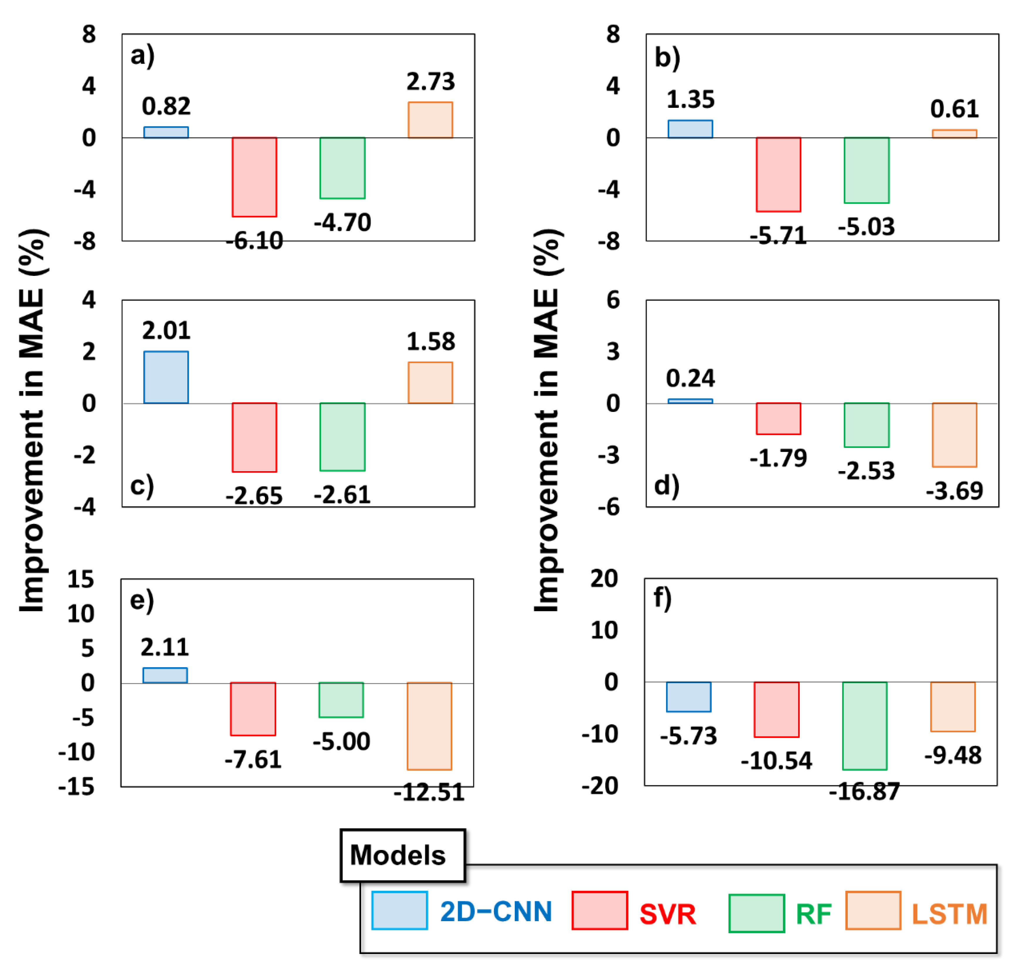
4.3. Investigation of Robustness of Models
5. Conclusions
Author Contributions
Funding
Institutional Review Board Statement
Informed Consent Statement
Data Availability Statement
Acknowledgments
Conflicts of Interest
References
- Brutsaert, W. Evaporation into the Atmosphere: Theory, History and Applications; Springer Science & Business Media: Berlin, Germany, 2013; Volume 1. [Google Scholar]
- Norman, J.M.; Kustas, W.P.; Humes, K.S. Source approach for estimating soil and vegetation energy fluxes in observations of directional radiometric surface temperature. Agric. For. Meteorol. 1995, 77, 263–293. [Google Scholar] [CrossRef]
- Emerson, C.W.; Anemone, R.L. Ongoing Developments in Geospatial Data, Software, and Hardware with Prospects for Anthropological Applications; Anemone, R.L., Ed.; University of New Mexico Press: Albuquerque, NM, USA, 2018; p. 21. [Google Scholar]
- Bégué, A.; Leroux, L.; Soumaré, M.; Faure, J.-F.; Diouf, A.A.; Augusseau, X.; Touré, L.; Tonneau, J.-P. Remote sensing products and services in support of agricultural public policies in Africa: Overview and challenges. Front. Sustain. Food Syst. 2020, 4, 58. [Google Scholar] [CrossRef]
- UN-GGIM. UN-GGIM (UN-Global Geospatial Information Management) Inter-Agency and Expert Group on the Sustainable Development Goal Indicators (IAEG-SDGS) Working Group Report on Geospatial Information; United Nations: New York, NY, USA, 2013. [Google Scholar]
- Anderson, M.; Kustas, W. Thermal remote sensing of drought and evapotranspiration. Eos Trans. Am. Geophys. Union 2008, 89, 233–234. [Google Scholar] [CrossRef]
- Chen, J.M.; Liu, J. Evolution of evapotranspiration models using thermal and shortwave remote sensing data. Remote Sens. Environ. 2020, 237, 111594. [Google Scholar] [CrossRef]
- Cui, Y.; Song, L.; Fan, W. Generation of spatio-temporally continuous evapotranspiration and its components by coupling a two-source energy balance model and a deep neural network over the Heihe River Basin. J. Hydrol. 2021, 597, 126176. [Google Scholar] [CrossRef]
- Fisher, J.B.; Melton, F.; Middleton, E.; Hain, C.; Anderson, M.; Allen, R.; McCabe, M.F.; Hook, S.; Baldocchi, D.; Townsend, P.A. The future of evapotranspiration: Global requirements for ecosystem functioning, carbon and climate feedbacks, agricultural management, and water resources. Water Resour. Res. 2017, 53, 2618–2626. [Google Scholar] [CrossRef]
- Zhang, K.; Kimball, J.S.; Running, S.W. A review of remote sensing based actual evapotranspiration estimation. Wiley Interdiscip. Rev. Water 2016, 3, 834–853. [Google Scholar] [CrossRef]
- Khan, M.S.; Jeong, J.; Choi, M. An improved remote sensing based approach for predicting actual Evapotranspiration by integrating LiDAR. Adv. Space Res. 2021, 68, 1732–1753. [Google Scholar] [CrossRef]
- Norman, J.; Kustas, W.; Prueger, J.; Diak, G. Surface flux estimation using radiometric temperature: A dual-temperature-difference method to minimize measurement errors. Water Resour. Res. 2000, 36, 2263–2274. [Google Scholar] [CrossRef] [Green Version]
- Shang, K.; Yao, Y.; Liang, S.; Zhang, Y.; Fisher, J.B.; Chen, J.; Liu, S.; Xu, Z.; Zhang, Y.; Jia, K. DNN-MET: A deep neural networks method to integrate satellite-derived evapotranspiration products, eddy covariance observations and ancillary information. Agric. For. Meteorol. 2021, 308, 108582. [Google Scholar] [CrossRef]
- Wilson, K.B.; Hanson, P.J.; Mulholland, P.J.; Baldocchi, D.D.; Wullschleger, S.D. A comparison of methods for determining forest evapotranspiration and its components: Sap-flow, soil water budget, eddy covariance and catchment water balance. Agric. For. Meteorol. 2001, 106, 153–168. [Google Scholar] [CrossRef]
- Jiang, L.; Zhang, B.; Han, S.; Chen, H.; Wei, Z. Upscaling evapotranspiration from the instantaneous to the daily time scale: Assessing six methods including an optimized coefficient based on worldwide eddy covariance flux network. J. Hydrol. 2021, 596, 126135. [Google Scholar] [CrossRef]
- Wang, L.; Wu, B.; Elnashar, A.; Zeng, H.; Zhu, W.; Yan, N. Synthesizing a Regional Territorial Evapotranspiration Dataset for Northern China. Remote Sens. 2021, 13, 1076. [Google Scholar] [CrossRef]
- Delogu, E.; Olioso, A.; Alliès, A.; Demarty, J.; Boulet, G. Evaluation of Multiple Methods for the Production of Continuous Evapotranspiration Estimates from TIR Remote Sensing. Remote Sens. 2021, 13, 1086. [Google Scholar] [CrossRef]
- Khan, M.S.; Liaqat, U.W.; Baik, J.; Choi, M. Stand-alone uncertainty characterization of GLEAM, GLDAS and MOD16 evapotranspiration products using an extended triple collocation approach. Agric. For. Meteorol. 2018, 252, 256–268. [Google Scholar] [CrossRef]
- Khan, M.S.; Baik, J.; Choi, M. Inter-comparison of evapotranspiration datasets over heterogeneous landscapes across Australia. Adv. Space Res. 2020, 66, 533–545. [Google Scholar] [CrossRef]
- Nisa, Z.; Khan, M.S.; Govind, A.; Marchetti, M.; Lasserre, B.; Magliulo, E.; Manco, A. Evaluation of SEBS, METRIC-EEFlux, and QWaterModel Actual Evapotranspiration for a Mediterranean Cropping System in Southern Italy. Agronomy 2021, 11, 345. [Google Scholar] [CrossRef]
- Falge, E.; Baldocchi, D.; Olson, R.; Anthoni, P.; Aubinet, M.; Bernhofer, C.; Burba, G.; Ceulemans, R.; Clement, R.; Dolman, H. Gap filling strategies for defensible annual sums of net ecosystem exchange. Agric. For. Meteorol. 2001, 107, 43–69. [Google Scholar] [CrossRef] [Green Version]
- Stauch, V.J.; Jarvis, A.J. A semi-parametric gap-filling model for eddy covariance CO2 flux time series data. Glob. Chang. Biol. 2006, 12, 1707–1716. [Google Scholar] [CrossRef]
- Hui, D.; Wan, S.; Su, B.; Katul, G.; Monson, R.; Luo, Y. Gap-filling missing data in eddy covariance measurements using multiple imputation (MI) for annual estimations. Agric. For. Meteorol. 2004, 121, 93–111. [Google Scholar] [CrossRef]
- Foltýnová, L.; Fischer, M.; McGloin, R.P. Recommendations for gap-filling eddy covariance latent heat flux measurements using marginal distribution sampling. Theor. Appl. Climatol. 2020, 139, 677–688. [Google Scholar] [CrossRef]
- Safa, B.; Arkebauer, T.J.; Zhu, Q.; Suyker, A.; Irmak, S. Net Ecosystem Exchange (NEE) simulation in maize using artificial neural networks. IFAC J. Syst. Control 2019, 7, 100036. [Google Scholar] [CrossRef]
- Cui, Y.; Ma, S.; Yao, Z.; Chen, X.; Luo, Z.; Fan, W.; Hong, Y. Developing a gap-filling algorithm using DNN for the Ts-VI triangle model to obtain temporally continuous daily actual evapotranspiration in an arid area of China. Remote Sens. 2020, 12, 1121. [Google Scholar] [CrossRef] [Green Version]
- Wutzler, T.; Lucas-Moffat, A.; Migliavacca, M.; Knauer, J.; Sickel, K.; Šigut, L.; Menzer, O.; Reichstein, M. Basic and extensible post-processing of eddy covariance flux data with REddyProc. Biogeosciences 2018, 15, 5015–5030. [Google Scholar] [CrossRef] [Green Version]
- Pastorello, G.; Trotta, C.; Canfora, E.; Chu, H.; Christianson, D.; Cheah, Y.-W.; Poindexter, C.; Chen, J.; Elbashandy, A.; Humphrey, M. The FLUXNET2015 dataset and the ONEFlux processing pipeline for eddy covariance data. Sci. Data 2020, 7, 225. [Google Scholar] [CrossRef] [PubMed]
- van Wijk, M.T.; Bouten, W. Water and carbon fluxes above European coniferous forests modelled with artificial neural networks. Ecol. Model. 1999, 120, 181–197. [Google Scholar] [CrossRef]
- Schmidt, A.; Wrzesinsky, T.; Klemm, O. Gap Filling and Quality Assessment of CO2 and Water Vapour Fluxes above an Urban Area with Radial Basis Function Neural Networks. Bound.-Layer Meteorol. 2008, 126, 389–413. [Google Scholar] [CrossRef]
- Moffat, A.M.; Papale, D.; Reichstein, M.; Hollinger, D.Y.; Richardson, A.D.; Barr, A.G.; Beckstein, C.; Braswell, B.H.; Churkina, G.; Desai, A.R.; et al. Comprehensive comparison of gap-filling techniques for eddy covariance net carbon fluxes. Agric. For. Meteorol. 2007, 147, 209–232. [Google Scholar] [CrossRef]
- Sun, H.; Xu, Q. Evaluating Machine Learning and Geostatistical Methods for Spatial Gap-Filling of Monthly ESA CCI Soil Moisture in China. Remote Sens. 2021, 13, 2848. [Google Scholar] [CrossRef]
- Sarafanov, M.; Kazakov, E.; Nikitin, N.O.; Kalyuzhnaya, A.V. A Machine Learning Approach for Remote Sensing Data Gap-Filling with Open-Source Implementation: An Example Regarding Land Surface Temperature, Surface Albedo and NDVI. Remote Sens. 2020, 12, 3865. [Google Scholar] [CrossRef]
- Bianco, M.J.; Gerstoft, P.; Traer, J.; Ozanich, E.; Roch, M.A.; Gannot, S.; Deledalle, C.-A. Machine learning in acoustics: Theory and applications. J. Acoust. Soc. Am. 2019, 146, 3590–3628. [Google Scholar] [CrossRef] [Green Version]
- Yu, T.-C.; Fang, S.-Y.; Chiu, H.-S.; Hu, K.-S.; Tai, P.H.-Y.; Shen, C.C.-F.; Sheng, H. Pin accessibility prediction and optimization with deep learning-based pin pattern recognition. IEEE Trans. Comput.-Aided Des. Integr. Circuits Syst. 2020, 40, 2345–2356. [Google Scholar] [CrossRef]
- Peppert, F.; von Kleist, M.; Schütte, C.; Sunkara, V. On the sufficient condition for solving the gap-filling problem using deep convolutional neural networks. IEEE Trans. Neural Netw. Learn. Syst. 2021. [Google Scholar] [CrossRef] [PubMed]
- Nguyen, P.; Halem, M. Deep Learning Models for Predicting CO2 Flux Employing Multivariate Time Series; Mile TS: Anchorage, AK, USA, 2019. [Google Scholar]
- Huang, I.; Hsieh, C.-I. Gap-Filling of Surface Fluxes Using Machine Learning Algorithms in Various Ecosystems. Water 2020, 12, 3415. [Google Scholar] [CrossRef]
- Kwon, H.-J.; Lee, J.-H.; Lee, Y.-K.; Lee, J.-W.; Jung, S.-W.; Kim, J. Seasonal variations of evapotranspiration observed in a mixed forest in the Seolmacheon catchment. Korean J. Agric. For. Meteorol. 2009, 11, 39–47. [Google Scholar] [CrossRef] [Green Version]
- Paszke, A.; Gross, S.; Massa, F.; Lerer, A.; Bradbury, J.; Chanan, G.; Killeen, T.; Lin, Z.; Gimelshein, N.; Antiga, L. Pytorch: An imperative style, high-performance deep learning library. Adv. Neural Inf. Process. Syst. 2019, 32, 8026–8037. [Google Scholar]
- Chirodea, M.C.; Novac, O.C.; Novac, C.M.; Bizon, N.; Oproescu, M.; Gordan, C.E. Comparison of Tensorflow and PyTorch in Convolutional Neural Network-based Applications. In Proceedings of the 2021 13th International Conference on Electronics, Computers and Artificial Intelligence (ECAI), Pitesti, Romania, 1–3 July 2021; pp. 1–6. [Google Scholar]
- Banda, P.; Cemek, B.; Küçüktopcu, E. Estimation of daily reference evapotranspiration by neuro computing techniques using limited data in a semi-arid environment. Arch. Agron. Soil Sci. 2018, 64, 916–929. [Google Scholar] [CrossRef]
- Liu, Z. A method of SVM with normalization in intrusion detection. Procedia Environ. Sci. 2011, 11, 256–262. [Google Scholar] [CrossRef] [Green Version]
- Albawi, S.; Mohammed, T.A.; Al-Zawi, S. Understanding of a convolutional neural network. In Proceedings of the 2017 International Conference on Engineering and Technology (ICET), Antalya, Turkey, 21–23 August 2017; pp. 1–6. [Google Scholar]
- Kim, P. Convolutional neural network. In MATLAB Deep Learning; Springer: Berkeley, CA, USA, 2017; pp. 121–147. [Google Scholar]
- Cortes, C.; Vapnik, V. Support-vector networks. Mach. Learn. 1995, 20, 273–297. [Google Scholar] [CrossRef]
- Kim, Y.; Johnson, M.S.; Knox, S.H.; Black, T.A.; Dalmagro, H.J.; Kang, M.; Kim, J.; Baldocchi, D. Gap-filling approaches for eddy covariance methane fluxes: A comparison of three machine learning algorithms and a traditional method with principal component analysis. Glob. Chang. Biol. 2020, 26, 1499–1518. [Google Scholar] [CrossRef]
- Breiman, L. Random forests. Mach. Learn. 2001, 45, 5–32. [Google Scholar] [CrossRef] [Green Version]
- Yang, Y.; Dong, J.; Sun, X.; Lima, E.; Mu, Q.; Wang, X. A CFCC-LSTM model for sea surface temperature prediction. IEEE Geosci. Remote Sens. Lett. 2017, 15, 207–211. [Google Scholar] [CrossRef]
- Jeong, M.-H.; Lee, T.-Y.; Jeon, S.-B.; Youm, M. Highway Speed Prediction Using Gated Recurrent Unit Neural Networks. Appl. Sci. 2021, 11, 3059. [Google Scholar] [CrossRef]
- Jeon, S.-B.; Jeong, M.-H.; Lee, T.-Y.; Lee, J.-H.; Cho, J.-M. Bus Travel Speed Prediction Using Long Short-term Memory Neural Network. Sens. Mater 2020, 32, 4441–4447. [Google Scholar] [CrossRef]
- Hochreiter, S.; Schmidhuber, J. Long short-term memory. Neural Comput. 1997, 9, 1735–1780. [Google Scholar] [CrossRef]
- Alcântara, E.H.; Stech, J.L.; Lorenzzetti, J.A.; Bonnet, M.P.; Casamitjana, X.; Assireu, A.T.; de Moraes Novo, E.M.L. Remote sensing of water surface temperature and heat flux over a tropical hydroelectric reservoir. Remote Sens. Environ. 2010, 114, 2651–2665. [Google Scholar] [CrossRef]
- Cui, Y.; Liu, Y.; Gan, G.; Wang, R. Hysteresis behavior of surface water fluxes in a hydrologic transition of an ephemeral Lake. J. Geophys. Res. Atmos. 2020, 125, e2019JD032364. [Google Scholar] [CrossRef]
- Dhungel, R.; Aiken, R.; Evett, S.R.; Colaizzi, P.D.; Marek, G.; Moorhead, J.E.; Baumhardt, R.L.; Brauer, D.; Kutikoff, S.; Lin, X. Energy Imbalance and Evapotranspiration Hysteresis Under an Advective Environment: Evidence From Lysimeter, Eddy Covariance, and Energy Balance Modeling. Geophys. Res. Lett. 2021, 48, e2020GL091203. [Google Scholar] [CrossRef]
- Zhang, Q.; Manzoni, S.; Katul, G.; Porporato, A.; Yang, D. The hysteretic evapotranspiration—Vapor pressure deficit relation. J. Geophys. Res. Biogeosciences 2014, 119, 125–140. [Google Scholar] [CrossRef]
- Lin, R.; Liu, S.; Yang, M.; Li, M.; Zhou, M.; Li, S. Hierarchical recurrent neural network for document modeling. In Proceedings of the 2015 Conference on Empirical Methods in Natural Language Processing, Lisbon, Portugal, 17–21 September 2015; pp. 899–907. [Google Scholar]
- Rodriguez, P.; Wiles, J.; Elman, J.L. A recurrent neural network that learns to count. Connect. Sci. 1999, 11, 5–40. [Google Scholar] [CrossRef] [Green Version]
- Taylor, K.E. Summarizing multiple aspects of model performance in a single diagram. J. Geophys. Res. Atmos. 2001, 106, 7183–7192. [Google Scholar] [CrossRef]
- Chai, T.; Draxler, R.R. Root mean square error (RMSE) or mean absolute error (MAE). Geosci. Model Dev. Discuss. 2014, 7, 1525–1534. [Google Scholar]
- Miller, R.G., Jr. Beyond ANOVA: Basics of Applied Statistics; CRC Press: Boca Raton, FL, USA, 1997. [Google Scholar]
- Razali, N.M.; Wah, Y.B. Power comparisons of shapiro-wilk, kolmogorov-smirnov, lilliefors and anderson-darling tests. J. Stat. Modeling Anal. 2011, 2, 21–33. [Google Scholar]
- Yue, W.; Xu, J.; Tan, W.; Xu, L. The relationship between land surface temperature and NDVI with remote sensing: Application to Shanghai Landsat 7 ETM+ data. Int. J. Remote Sens. 2007, 28, 3205–3226. [Google Scholar] [CrossRef]
- Tarigan, S.; Stiegler, C.; Wiegand, K.; Knohl, A.; Murtilaksono, K. Relative contribution of evapotranspiration and soil compaction to the fluctuation of catchment discharge: Case study from a plantation landscape. Hydrol. Sci. J. 2020, 65, 1239–1248. [Google Scholar] [CrossRef]
- Khan, M.S.; Baik, J.; Choi, M. A physical-based two-source evapotranspiration model with Monin–Obukhov similarity theory. GIScience Remote Sens. 2021, 58, 88–119. [Google Scholar] [CrossRef]
- Wang, K.; Wang, P.; Li, Z.; Cribb, M.; Sparrow, M. A simple method to estimate actual evapotranspiration from a combination of net radiation, vegetation index, and temperature. J. Geophys. Res. Atmos. 2007, 112, D15107. [Google Scholar] [CrossRef]


| Site | Location | Study Period | Elevation (Measurement Height) 1 (m) | Canopy Height 2 (m) | Vegetation Type | Mean Annual Temperature (°C) | Mean Annual Precipitation (mm) | References | |
|---|---|---|---|---|---|---|---|---|---|
| Country | Latitude/Longitude (°N/°E) | ||||||||
| Seolmacheon (SMC) | South Korea | 37.94/126.96 | 2008 | 293 (19.2) | 15.0 | Mixed forest | 10.4 | 1332 | [39] |
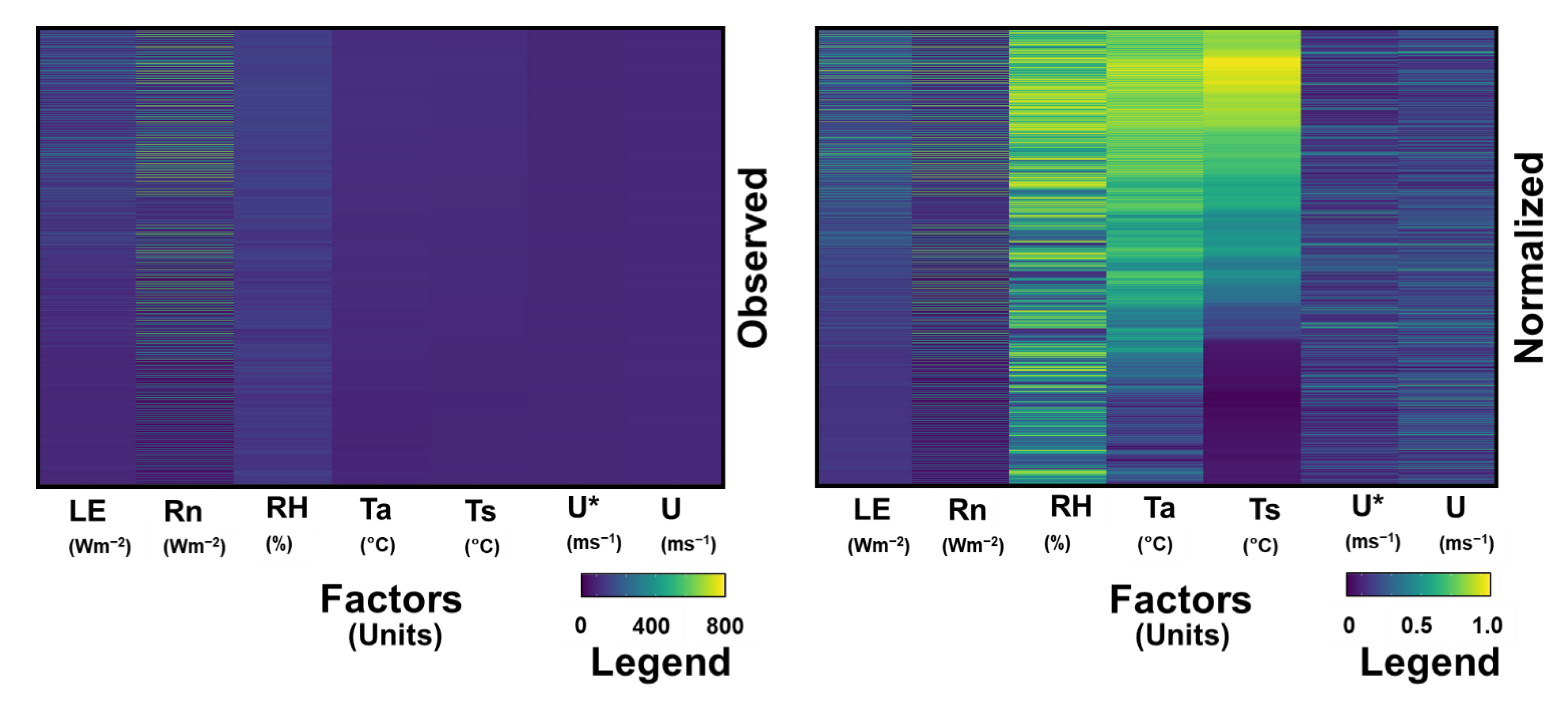
| Input Factors | Abbreviations | Definitions |
|---|---|---|
| Meteorological factors | U(t) | Wind speed at time t (m/s) |
| RH(t) | Relative humidity at time t (%) | |
| Rn(t) | Net radiation at time t (Wm−2) | |
| Ta(t) | Air temperature at time t (°C) | |
| U*(t) | Friction velocity at time t (m/s) | |
| Ts(t) | Surface temperature at time t (°C) | |
| Hysteresis factors | U(t − x) | Wind speed at time t − x (where the variable x is a multiplier and represents 30 min before time t) |
| For CNN model x = 2, 6, 12, 18, 24 | ||
| For LSTM model x = 1, 3, 6, 9, 12 | ||
| RH(t − x) | Relative humidity at time t − x | |
| For CNN model x = 2, 6, 12, 18, 24 | ||
| For LSTM model x = 1, 3, 6, 9, 12 | ||
| Rn(t − x) | Net radiation at time t − x | |
| For CNN model x = 2, 6, 12, 18, 24 | ||
| For LSTM model x = 1, 3, 6, 9, 12 | ||
| Ta(t − x) | Air temperature at time t − x | |
| For CNN model x = 2, 6, 12, 18, 24 | ||
| For LSTM model x = 1, 3, 6, 9, 12 | ||
| U*(t − x) | Friction velocity at time t − x | |
| For CNN model x = 2, 6, 12, 18, 24 | ||
| For LSTM model x = 1, 3, 6, 9, 12 | ||
| Ts (t − x) | Surface temperature at time t − x | |
| For CNN model x = 2, 6, 12, 18, 24 | ||
| For LSTM model x = 1, 3, 6, 9, 12 | ||
| LE (t − x) | Latent heat flux at time t − x | |
| For CNN model x = 2, 6, 12, 18, 24 | ||
| For LSTM model x = 1, 3, 6, 9, 12 | ||
| For SVM model x = 1, 2, 3, 4, 5, 6 | ||
| For RF model x = 1, 2, 3, 4, 5, 6 |
| Country | Site Name | Model Name | Optimal Input Combinations |
|---|---|---|---|
| South Korea | Seolmacheon (SMC) forest site | CNN | U(t), RH(t), Rn(t), Ta(t), U*(t), Ts(t), U(t − 2), RH(t − 2), Rn(t − 2), Ta(t − 2), U*(t − 2), Ts(t − 2), LE(t − 2) |
| SVM | U(t), RH(t), Rn(t), Ta(t), U*(t), Ts(t), LE(t − 1) | ||
| RF | U(t), RH(t), Rn(t), Ta(t), U*(t), Ts(t), LE(t − 1) | ||
| LSTM | U(t), RH(t), Rn(t), Ta(t), U*(t), Ts(t), U(t − 3), RH(t − 3), Rn(t − 3), Ta(t − 3), U*(t − 3), Ts(t − 3), LE(t − 3) |
| Factors Included | Factors Eliminated | Models | MAE | RMSE | R2 |
|---|---|---|---|---|---|
| u*, Ts, Ta, Rh, RN | u | CNN | 37.54 | 55.96 | 0.76 |
| SVR | 38.46 | 57.14 | 0.76 | ||
| RF | 38.11 | 56.74 | 0.75 | ||
| LSTM | 38.18 | 57.37 | 0.74 | ||
| u, Ts, Ta, Rh, RN | u* | CNN | 37.34 | 55.85 | 0.76 |
| SVR | 38.32 | 58.82 | 0.76 | ||
| RF | 38.23 | 57.32 | 0.74 | ||
| LSTM | 39.01 | 57.85 | 0.73 | ||
| u, u*, Ta, Rh, RN | Ts | CNN | 37.09 | 55.85 | 0.76 |
| SVR | 37.21 | 57.34 | 0.78 | ||
| RF | 37.35 | 55.80 | 0.75 | ||
| LSTM | 38.63 | 58.08 | 0.73 | ||
| u, u*, Ts, Rh, RN | Ta | CNN | 37.76 | 56.41 | 0.76 |
| SVR | 36.90 | 55.86 | 0.77 | ||
| RF | 37.32 | 55.87 | 0.75 | ||
| LSTM | 40.70 | 60.13 | 0.71 | ||
| u, u*, Ts, Ta, RN | Rh | CNN | 37.05 | 55.54 | 0.76 |
| SVR | 39.01 | 58.71 | 0.77 | ||
| RF | 38.22 | 56.74 | 0.74 | ||
| LSTM | 44.16 | 63.83 | 0.68 | ||
| u, u*, Ts, Ta, Rh | RN | CNN | 40.02 | 61.05 | 0.71 |
| SVR | 40.07 | 62.18 | 0.75 | ||
| RF | 42.54 | 62.80 | 0.69 | ||
| LSTM | 42.97 | 64.88 | 0.67 |
Publisher’s Note: MDPI stays neutral with regard to jurisdictional claims in published maps and institutional affiliations. |
© 2021 by the authors. Licensee MDPI, Basel, Switzerland. This article is an open access article distributed under the terms and conditions of the Creative Commons Attribution (CC BY) license (https://creativecommons.org/licenses/by/4.0/).
Share and Cite
Khan, M.S.; Jeon, S.B.; Jeong, M.-H. Gap-Filling Eddy Covariance Latent Heat Flux: Inter-Comparison of Four Machine Learning Model Predictions and Uncertainties in Forest Ecosystem. Remote Sens. 2021, 13, 4976. https://doi.org/10.3390/rs13244976
Khan MS, Jeon SB, Jeong M-H. Gap-Filling Eddy Covariance Latent Heat Flux: Inter-Comparison of Four Machine Learning Model Predictions and Uncertainties in Forest Ecosystem. Remote Sensing. 2021; 13(24):4976. https://doi.org/10.3390/rs13244976
Chicago/Turabian StyleKhan, Muhammad Sarfraz, Seung Bae Jeon, and Myeong-Hun Jeong. 2021. "Gap-Filling Eddy Covariance Latent Heat Flux: Inter-Comparison of Four Machine Learning Model Predictions and Uncertainties in Forest Ecosystem" Remote Sensing 13, no. 24: 4976. https://doi.org/10.3390/rs13244976
APA StyleKhan, M. S., Jeon, S. B., & Jeong, M.-H. (2021). Gap-Filling Eddy Covariance Latent Heat Flux: Inter-Comparison of Four Machine Learning Model Predictions and Uncertainties in Forest Ecosystem. Remote Sensing, 13(24), 4976. https://doi.org/10.3390/rs13244976