Evaluating Image Normalization via GANs for Environmental Mapping: A Case Study of Lichen Mapping Using High-Resolution Satellite Imagery

Abstract

Illumination variations in non-atmospherically corrected high-resolution satellite (HRS) images acquired at different dates/times/locations pose a major challenge for large-area environmental mapping and monitoring. This problem is exacerbated in cases where a classification model is trained only on one image (and often limited training data) but applied to other scenes without collecting additional samples from these new images. In this research, by focusing on caribou lichen mapping, we evaluated the potential of using conditional Generative Adversarial Networks (cGANs) for the normalization of WorldView-2 (WV2) images of one area to a source WV2 image of another area on which a lichen detector model was trained. In this regard, we considered an extreme case where the classifier was not fine-tuned on the normalized images. We tested two main scenarios to normalize four target WV2 images to a source 50 cm pansharpened WV2 image: (1) normalizing based only on the WV2 panchromatic band, and (2) normalizing based on the WV2 panchromatic band and Sentinel-2 surface reflectance (SR) imagery. Our experiments showed that normalizing even based only on the WV2 panchromatic band led to a significant lichen-detection accuracy improvement compared to the use of original pansharpened target images. However, we found that conditioning the cGAN on both the WV2 panchromatic band and auxiliary information (in this case, Sentinel-2 SR imagery) further improved normalization and the subsequent classification results due to adding a more invariant source of information. Our experiments showed that, using only the panchromatic band, F1-score values ranged from 54% to 88%, while using the fused panchromatic and SR, F1-score values ranged from 75% to 91%.

1. Introduction

Remote sensing (RS) has been widely proven to be advantageous for various environmental mapping tasks [1,2,3,4,5]. Regardless of the RS data used for mapping, there are several challenges that can prevent the generation of accurate maps of land cover types of interest. Among these challenges, one is collecting sufficient training samples for a classification model. This is particularly true for classifiers that require large amounts of training data and/or if fieldwork is required in difficult-to-access sites. This challenge has been intensified lately due to COVID-19 restrictions worldwide. A second challenge is that suitable RS data for a study area may not be available; e.g., high spatial resolution (HSR) or cloud-free imagery. UAVs can be beneficial for overcoming both of these challenges due to their high flexibility (e.g., ability to quickly acquire imagery in study sites where other suitable RS data are not available), but planning UAV flights and processing UAV images over wide areas can be time and cost-prohibitive (although they are usually more efficient than acquiring traditional field data). A third challenge is that satellite/UAV images are subject to both spatial and temporal illumination variations (caused by variations in atmospheric conditions, sensor views, solar incidence angle, etc.) that may cause radiometric variations in image pixel values, especially in shortwave bands (e.g., Blue). Without accounting for illumination variations, the performance of classification models can be substantially degraded in unseen/test images. The main reason for this accuracy degradation is that the model learned from the distribution of the source image, which has now shifted in a given target image, meaning that it can no longer perform on the target image as well as it did on the source image on which it was trained. Such image-to-image variations are also found in images acquired by the same sensor unless appropriate normalizations and/or atmospheric corrections are performed.

In general, illumination variations in different scenes (including those acquired over the same area but different times) are a function of topography, the bidirectional reflectance distribution function (BRDF), and atmospheric effects. Accounting for these variables helps to balance radiometric variations in different images, thus making them consistent for different downstream tasks. In the case of raw images, one way of performing such corrections is through absolute radiometric correction to the surface reflectance, which consists of converting raw digital numbers to top-of-atmosphere (TOA) reflectance and then applying an atmospheric correction approach to derive ground-level surface reflectance. Relative radiometric correction (or normalization) is another way of harmonizing images that can be applied to cross-sensor images. Normalizing images to RS surface reflectance (SR) images (such as Landsat or Sentinel-2 images) [6,7,8] or to ground-measured SR [9] is a popular approach to harmonizing different sources of RS images. Maas and Rajan [6] proposed a normalization approach (called scatter-plot matching (SPM)) based on invariant features in the scatter plot of pixel values in the red and near-infrared (NIR) bands. The authors reported the successful application of their approach for normalizing Landsat-7 images to Landsat-5 images and for normalizing to SR, although this approach only considers the red and NIR bands. Abuelgasim and Leblanc [7] developed a workflow to generate Leaf Area Index (LAI) products (with an emphasis on northern parts of Canada). In this regard, the authors employed different sources of RS imagery (including Landsat, AVHRR, and SPOT VGT). To normalize Landsat-7 and Landsat-5 images to AVHRR and SPOT VGT images, the authors trained a Theil–Sen regression model using all the common pixels in a pair of images (i.e., the reference and target images) through improving the efficiency of the original approach to be able to process much more common pixels. In a study by Macander [8], a solution was developed to normalize 2 m Pleiades satellite imagery to Landsat-8 SR imagery. The authors aimed to match the blue, green, red, and NIR bands to the same bands of a Landsat-8 SR composite (a 5 year summertime composite). For this purpose, they first masked out pixels with highly dynamic reflectance. Then, a linear regression was established between the Landsat-8 composite and the aggregated 30 m Pleiades satellite imagery. Finally, the trained linear model was applied directly to the 2 m Pleiades satellite imagery to obtain a high-resolution SR product. Rather than calibrating images based on an SR image, Staben, et al. [9] calibrated WorldView-2 (WV2) images to ground SR measurements. For this, the authors used a quadratic equation to convert TOA spectral radiance in WV2 imagery to average field spectra for different target features (e.g., grass, water, sand, etc.). The experiments in that study showed that there was an acceptable level of discrepancies between the ground-truth averaged field spectra and the calibrated bands of the WV2 image, with the NIR band resulting in the largest variance among the other bands.

Although these normalization techniques have proven to be useful for making different non-atmospherically corrected images consistent with atmospherically corrected images, they should be done separately for each image (mainly through non-linear regression modeling). Such approaches are advantageous to harmonize images that have different characteristics (e.g., different acquisition frequencies). However, due to surface illumination variations (depending on sun angle) and varying atmospheric conditions, this does not guarantee seamless scene-to-scene spectral consistency [8].

Another way of harmonizing images is based on classic approaches such as histogram matching (HM) [10]. HM is an efficient, context-unaware technique that is widely used to transform the histogram of a given image to match a specific histogram (e.g., the histogram of another image) [10]. Although this approach is efficient and easy to apply, it does not take into account contextual and textural information. Moreover, HM-based methods do not result in reasonable normalizations when the histogram of the target image is very different from that of the source image [11]. All the approaches described above intuitively aim to adapt a source domain to a target domain, which in the literature is known as the adaptation of data distributions, a subfield of Domain Adaptation (DA) [12]. The emergence of Deep Learning (DL) has opened new insights into how DA can significantly improve the performance of models on target images. DA has several variants, but they can be mainly grouped into two classes: Supervised DA (SDA) and Unsupervised DA (UDA) [13]. DL-based DA approaches have also been successfully employed in RS applications, mainly for urban mapping [14].

In this study, the main focus is not on normalizing images to surface reflectance, but rather on harmonizing different images regardless of their preprocessing level (e.g., radiometrically corrected, TOA reflectance, surface reflectance), which is a case of UDA. Considering this general-purpose direction, orthogonal to the majority of research in the context of environmental RS, we investigated an extreme case that has not been well studied in environmental RS mapping. The central question addressed in this study is that, if we assume that a classifier (either a DL model or a conventional one, or either a pixel- or object based) has already been trained on a single HRS image of one area (in our case, WV2 imagery), and if we do not have access to any of the target images of other areas during model training, to what degree is it possible to apply the same model, without any further training or collections of new samples whatsoever, to unseen target images and still obtain reasonable accuracy? This is a special, extreme case of UDA (or as we call it in this paper, image normalization). In recent years, Generative Adversarial Networks (GANs) [15] have been used for several applications (e.g., DA, super-resolution, image fusion, semantic segmentation, etc.) in the context of RS [16,17,18]. Given the potential of GANs in different vision tasks, cGANs based on Pix2Pix [19] were adopted as the base of image normalization in this study.

2. Methodology

The backbone of the framework applied in this research is based on cGANs [20]. More precisely, the framework revolves around supervised image-to-image translation. In this regard, the goal is to normalize target images based on a source image (on which the classifier was trained). The methodology aimed to normalize target images using a cGAN to a source image to allow for the more accurate mapping of target images without collecting additional training data. There are some considerations when it comes to applying a cGAN for image normalization. First, the source image selected should contain most of the land cover types that are spectrally similar to the land covers of interest that could appear in the target images. Second, the classification model should be trained well on the source image given the fact that sufficient training data for target images may not be available. Third, none of the target images had been seen or used (even in an unsupervised manner) in any part of model training process; that is, no prior knowledge on target images was available, except that they could be different from the source image in terms of illumination conditions. These considerations led to an extreme situation which could also be a common problem in real-world mapping tasks, as collecting training samples is expensive, fine-tuning classifiers may not be effective, processing multiple data sets synchronously may not be computationally feasible, context-unaware data augmentation techniques may not be effective, etc.

cGAN Framework

In the field of RS, image-to-image translation has several applications. For example, one interesting application is to synthesize optical RS images (e.g., RGB images) based on non-optical RS data (e.g., SAR images) [21]. Another application of image translation in RS is image colorization, in which the goal is to colorize gray-scale images [22]. Image colorization can be performed using different solutions such as GANs that aim to approximate a distribution for the outputs that is similar to the distribution of the training data. This important feature allows GANs to generate synthetic images that are more similar—also in terms of color—to real images. In the case of RS images, it is generally not sufficient to have images that are colorful; in other words, we need images in which the different types of land cover are assigned semantically realistic colors, although visually assessing this beyond the RGB bands is difficult. In addition to this challenge, in some mapping tasks (such as caribou lichen mapping) using RS data, spectral information could typically be more important than geometric information, which is generally more crucial in natural images. Therefore, if a classifier already trained on real images is applied to synthesized RS images, it would have difficulty detecting land cover of interest in cases where color information is not consistent with real images.

Given the aforementioned challenges, we adopted Pix2Pix [19] with some modifications as the backbone for cGAN in this study. Before elaborating on Pix2Pix, it is required to briefly review vanilla GANs. GANs adversarially train a generative model (aiming to approximate real data distribution) and a discriminative model (aiming to distinguish a real sample from a fake one generated by the generative model) [15]. Since these two models are optimized simultaneously, they are trained in a two-player minmax game manner, in which the goal is to minimize the loss of the generative model and maximize the loss of the discriminative model. Since vanilla GANs restrict the user from controlling the generator (and the images generated accordingly), their applications are limited. To expand the range of their applications, conditional GANs (cGANs) were introduced that condition both the generator and discriminator based on an additional source of information (e.g., class labels, another image source, etc.). Given this, the objective function of cGANs can be defined as Equation (1) [20].

$${ℒ}_{cGAN}\left(D, G\right)={𝔼}_{{x, y\sim p}_{data}(x, y)} \left[\log D\left(x, y\right)\right]+{𝔼}_{{x\sim p}_{data}{\left(x\right), z\sim p}_z\left(z\right)} \left[\log \left(1 - D\left(x, G\left(x, z\right)\right)\right)\right]$$

(1)

where the goal is to map the random noise vector z to target y given x using a discriminator D(.) and a generator G(.) trained in an adversarial manner.

The use of Equation (1) alone may not result in fine-grained translated images. To remedy this, Pix2Pix uses an L1 loss (Equation (2)) besides Equation (1) in its objective function to improve the spatial fidelity of the synthesized images.

$${ℒ}_{L1}\left(G\right)={𝔼}_{{x, y\sim p}_{data}{(x, y), z\sim p}_z\left(z\right)}\left[{\parallel y - G(x, z)\parallel }_1\right]$$

(2)

where y is the target, G(.) is the generator, and $\parallel { .\parallel }_1$ is the L1 norm calculated based on the target and the output generated by the generator. The reason for using the L1 norm rather than L2 norm is that L1 helps to generate less blurry images [23]. Combining the adversarial loss and L1 loss, we can define the objective function of Pix2Pix as Equation (3).

$${ℒ}_{Pix2Pix}{=ℒ}_{cGAN}{+\lambda }_1{ℒ}_{L1}$$

(3)

To improve the training of GANs (i.e., mitigating the vanishing gradients problem), we used conditional Least Squares GANs (cLSGANs) [24] (Equation (4)). In contrast to the vanilla GANs, whose discriminator is a classifier with the sigmoid cross entropy loss function, cLSGAN does not apply a sigmoid function, and thus treats the output as a regression and minimizes the least squares of errors in the objective function.

$$\begin{array}{l}{ℒ}_{cLSGAN}\left(D\right)=\frac{1}{2}{𝔼}_{{x, y\sim p}_{data}(x, y)} \left[{\left(D(x, y) - 1\right)}^2\right]+\frac{1}{2}{𝔼}_{{x\sim p}_{data}{\left(x\right), z\sim p}_z\left(z\right)} \left[{D(x, G(x, z\left)\right)}^2\right],\\ {ℒ}_{cLSGAN}\left(G\right)=\frac{1}{2}{𝔼}_{{x\sim p}_{data}{\left(x\right), z\sim p}_z\left(z\right)} \left[{\left(D\left(G\right(x, z\left)\right) - 1\right)}^2\right].\end{array}$$

(4)

In addition to the use of the original loss function of Pix2Pix, we also tested whether adding a perceptual loss can provide better color consistency in the normalization process. For this purpose, we used a pretrained VGG19 trained on the ImageNet dataset. Since this model takes in only RGB images, we replaced the input layer and then fine-tuned it on an urban classification task using WorldView-2 images to better adapt it to our application/data in this study [25]. The perceptual loss was used to calculate the Euclidean distance between the VGG19-derived feature maps of the generated and real images (Equation (5)).

$${ℒ}_{Perceptual}={𝔼}_{{x, y\sim p}_{data}{(x, y), z\sim p}_z\left(z\right)}\left[\parallel {\Phi }_{i,j}\left(y\right) {- \Phi }_{i,j}{\left(G(x, z\right)\parallel }_2^2\right],$$

(5)

where Φ_i,j is the j-th convolution (after activation) before the i-th maxpooling layer of the VGG16. In this study, we calculated the perceptual loss based on the feature maps of the fourth convolution before the fifth maxpooling layer. Besides the perceptual loss, we added the total variation (TV) loss (Equation (6)), which is the is the sum of the absolute differences for neighboring pixel-values in the generated image, to reduce noise (such as chessboard-like artifacts) in the generated images.

$${ℒ}_{TV}={\displaystyle \sum }_{i=1, j=1}^{H, W}\left[{\left({G(x ,z)}_{i ,j+1}{- G(x, z)}_{i, j}\right)}^2+{\left({G(x, z)}_{i+1,j}{- G(x ,z)}_{i,j}\right)}^2\right],$$

(6)

where H and W are the height and width of the generated image.

As a result, the final loss function of the modified Pix2Pix (Pix2Pix+) in this study can be expressed as Equation (7).

$${ℒ}_{Pix2Pix+}{=ℒ}_{cLSGAN}{+\lambda }_1{ℒ}_{L1}{+\lambda }_2{ℒ}_{Perceptual }{+\lambda }_3{ℒ}_{TV},$$

(7)

where λ are the weights of the image space, perceptual, and TV losses, which were empirically chosen to be 100, 1, and 10, respectively.

As with the original Pix2Pix, we used a patch-wise discriminator to model a high-frequency structure along with a low-frequency structure. For the generator, we used a U-Net model pretrained on the same urban classification task that the feature extractor VGG19 was fine-tuned on. The architecture of the generator is presented in Figure 1. The input size of images was chosen to be 256 × 256 pixels. A kernel size of 4 × 4 with a stride of 2 in the convolutional layers of both the encoding and decoding layers was employed. In the encoding layers, LeakyReLU activation with a slope of 0.2 was used, whereas in the decoding layers, ReLU activation was used. An Adam solver with the momentum parameters β₁ = 0.5 and β₁ = 0.999 and a learning rate of 0.0002 was used to train the cGANs for 300 epochs.

3. Experimental Design

To evaluate the potential of image normalization based on cGANs, we conducted an experimental test for caribou lichen cover mapping. Caribou are known as ecologically important animals, but due to multiple factors ranging from climate change to hunting and disease, global caribou populations have been declining in recent decades, and they are now on the International Union for the Conservation of Nature’s (IUCN) red list of threatened species [26]. Land cover change in caribou habitats is a major factor affecting resource availabilities, and it is driven by both indirect impacts of anthropogenic activities (e.g., climate change causing vegetation changes) as well as direct impacts (e.g., deforestation or forest degradation) [27]. When land cover changes occur, it may cause caribou herds to change their distributions and migration patterns when foraging for food [28]. Thus, for caribou conservation efforts, it is important to monitor and analyze the resources on which caribou are highly dependent, such as lichen, which is the main source of winter food of caribou [29,30]. Caribou lichens are generally bright-colored and could be challenging to detect in the case of illumination variations between a source image and target images, especially where there are other non-lichen bright features. To evaluate cGANs for image normalization for the lichen mapping task, we used WV2 images with a spatial resolution of 2 m for the multi-spectral bands and of 50 cm for the panchromatic band. Since WV2 images were subject to different atmospheric variations, it would also be reasonable to consider other sources of data/images that are less affected by atmospheric changes and lighting variations accordingly. A helpful option is to use atmospherically corrected images as auxiliary information to help cGANs to learn more stable features when normalizing target images. As explained in the next section, we also tested the potential of using both WV2 images and Sentinel-2 surface reflectance (SR) images for normalization.

3.1. Dataset

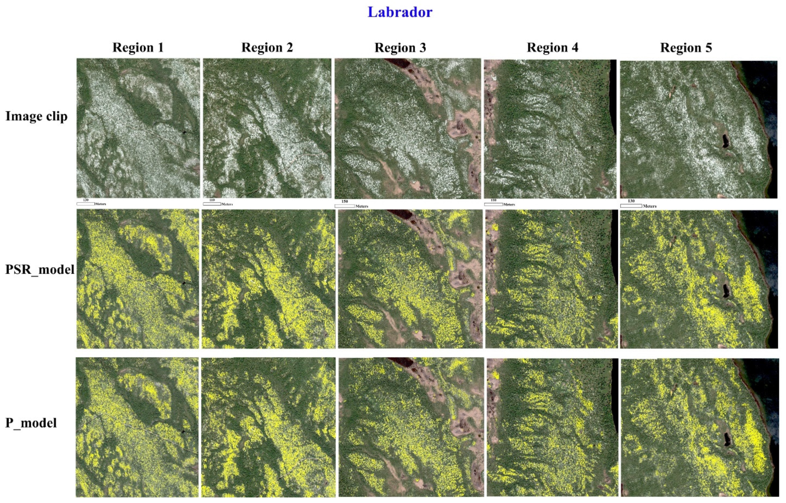
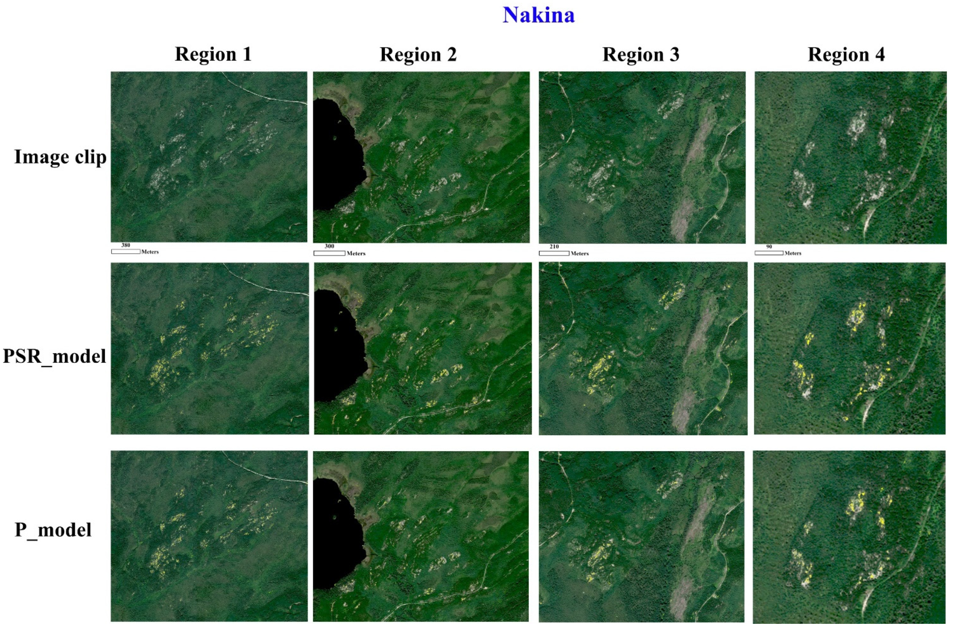
Five radiometrically corrected WV2 scenes with eight spectral bands from different parts of Canada were chosen for this study (Figure 2). The radiometric correction on raw data was performed by the vendor to mitigate image artifacts (appearing as streaks and banding in the raw images) through including a dark offset subtraction and a non-uniformity correction including detector-to-detector relative gain. The Manic-5 image covers a 405 km² area located south of the Manicouagan Reservoir, Québec, Canada around the Manic-5 dam. This area consists of boreal forest (black spruce dominated) and open lichen woodlands, or forests with lichen. There are many waterbodies and water courses. The Fire Lake image covers a 294 km² area located around the Fire Lake Iron Mine in Québec, Canada. This area is comprised of dense boreal forests (black spruce dominated) with a great proportion of open lichen woodlands and/or forests with lichen. The Labrador image was acquired over 273 km² located east of Labrador City, Labrador, Canada. This area is comprised of dense boreal forests (black spruce dominated) with open lichen woodlands and/or forests with lichen. There are also a significant number of water features (bodies and courses) in this area. The Churchill Falls image covers a 397 km² area located west of Churchill Falls, Labrador, Canada. This area is comprised of dense boreal forests (black spruce dominated), open lichen woodlands and/or forests with lichen. The Nakina image covers a 261 km² area located east of the township of Nakina, Ontario, Canada. This area is comprised of dense boreal forests with very sparse, small lichen patches. Like the other images, this image covers several water bodies.

We chose the image acquired over Manic-5 area as our source image from which the training data were collected and used to train the models on this study. The reason for choosing this image as our source image was that we conducted fieldwork within an area covered by this image. The other four images were used for testing the efficacy of the pipeline applied. We attempted to choose target images from our database that were different from our source image in terms of illumination as much as possible. In all the images except the Labrador image, there were clouds or haze that caused a shift in the distribution of data. Of the four target images, the Nakina image had the least lichen cover. The Fire Lake image was used as a complementary target image to visually evaluate some of the important sources of errors that were observed mainly in this image. Along with WV2 images, we also used Sentinel-2 SR images in this paper. We used the Sentinel-2 Level-2 A product, which is geometrically and atmospherically corrected from the TOA product through an atmospheric correction using a set of look-up tables based on libRadtran [31]. We chose six bands (B2-5, B8, B11) of 10 m Sentinel-2 SR cloud-free median composites (within the time periods close to the acquisition years of the WV2 images) and downloaded them from Google Earth Engine.

3.2. Training and Test Data

To train the cGANs, we used 5564 image patches with a size of 256 × 256 pixels. No specific preprocessing was performed on the images before inputting them into the models. In order to test the framework applied in this study, we clipped some sample parts of the Labrador, Churchill Falls, and Nakina images. A total of 14 regions in these three target images were clipped for testing purposes. From each of these 14 test image clips, through visual interpretation (with assistance from experts familiar with the areas), we randomly sampled at least 500 pixels (

Table 1. Number of samples collected from each region of the Labrador, Churchill Falls, and Nakina images.

Image	Region 1	Region 2	Region 3	Region 4	Region 5
Labrador	1020	808	1671	1015	1769
Churchill Falls	1284	740	899	1078	1063
Nakina	799	842	515	571	-

), given the extent of each clip. We attempted to equalize the number of lichen and background samples. Overall, 14,074 test pixels were collected from these three target images.

3.3. Normalization Scenarios

Different normalization scenarios were considered in this study based on either WV2 images or a combination of WV2 and auxiliary images. In fact, since WV2 images alone may not be sufficient to reach high-fidelity normalized target images (and accurate lichen mapping accordingly), we also used an auxiliary RS image, namely Sentinel-2 SR imagery, in this study. Given this, the goal was to normalize target WV2 images to a source eight-band pansharpened image with a spatial resolution of 50 cm. This means that the output of the normalization methods should be 50 cm to correspond to the source image. Using these two data sets, we considered four scenarios (Figure 3) for normalization as follows:

1.

Normalization based on the 2 m resolution WV2 multi-spectral bands (resampled to 50 cm);

2.

Normalization based on the WV2 panchromatic band concatenated/stacked with the 2 m multi-spectral bands (resampled to 50 cm);

3.

Normalization based on the WV2 panchromatic band alone;

4.

Normalization based on the WV2 panchromatic band concatenated/stacked with the Sentinel-2 SR imagery (resampled to 50 cm).

The scenarios 1, 3, and 4 can be considered as a special case of pan-sharpening where the spatial information comes from a target image but the spectral information comes from the source image. We performed two steps of experiments to evaluate the quality of image normalization using these scenarios. In the first step, we ruled out the scenarios that did not lead to realistic-looking results. In the second step, we used the approaches found practical in the first step to perform the main comprehensive quantitative tests on different target images.

3.3.1. Scenario 1: Normalization Based on 2 m Multi-Spectral Bands (Resampled to 50 cm)

One way of normalizing a target image to a source image is to follow a pseudo-super-resolution approach, in which the multi-spectral bands (in the case of WV2, with a spatial resolution of 2 m, which must be resampled to 50 cm to be processable by the model) are used as input to the cGAN. However, the difference here is that the goal now is to generate not only a higher-resolution image (with a spatial resolution of 50 cm), but also an image that has a similar spectral distribution to that of the source image. It should be noted that all the resampling to 50 cm was performed using a bi-linear technique before training the GANs.

3.3.2. Scenario 2: Normalization Based on the Panchromatic Band Concatenated/Stacked with 2 m Multi-Spectral Bands (Resampled to 50 cm)

The second way is to improve the spatial fidelity of the generated normalized image by incorporating higher-resolution information into the model without the use of a specialized super-resolution model. One such piece of information could be the panchromatic band, which has a much broader bandwidth than the individual multi-spectral or pansharpened data. In addition to its higher spatial resolution information, it can be hypothesized that this band alone has less variance than the multi-spectral bands combined under different atmospheric conditions. When adding the panchromatic band to the process, the model would learn high-resolution spatial information from the panchromatic band, and the spectral information from the multi-spectral bands. This scenario can be considered as a special type of pansharpening, except that in this case, the goal is to pansharpen a target image so that it not only has a higher spatial resolution, but also its spectral distribution is similar to that of the source image.

3.3.3. Scenario 3: Normalizing Based Only on the Panchromatic Band

The additional variance of multi-spectral bands among different scenes could degrade the performance of normalization in the second scenario. Since a panchromatic band is a high-resolution squeezed representation of the visible multi-spectral bands, it could also be tempting to experiment with the potential of using only this band without including the corresponding multi-spectral bands (to reduce the unwanted variance among different scenes) to analyze if normalization can also be properly conducted based only on this single band.

3.3.4. Scenario 4: Normalization Based on the Panchromatic Band Concatenated/Stacked with the Sentinel-2 Surface Reflectance Imagery (Resampled to 50 cm)

Theoretically, not including multi-spectral information in the third scenario has some downsides. For example, the model may not be able to learn sufficient features from the panchromatic band. On the other hand, the main shortcoming of the first and second scenarios is that the multi-spectral information can introduce higher spectral variance under different atmospheric conditions than the panchromatic band alone can. In this respect, based on the aforementioned factors, another way of approaching this problem is to use RS products that are atmospherically corrected. These can be SR products such as Sentinel-2 SR imagery. Despite having a much coarser resolution, it is hypothesized that combining the panchromatic band of the test image with the Sentinel-2 SR imagery can further improve normalization results by constraining the model to be less affected by abrupt atmosphere-driven changes in the panchromatic image. In this regard, the high-resolution information comes from the panchromatic band of the test image, and some invariant high-level spectral information comes from the corresponding Sentinel-2 SR image. To use SR imagery with the corresponding WV2 imagery, we first resampled the SR imagery to 50 cm using the bilinear technique and then co-registered the SR imagery to the WV2 using the AROSICS tool [32]. One of the main challenges in this scenario was the presence of clouds in the source image. There were two main problems in this respect. First, since we also used cloud-free Sentinel-2 imagery, the corresponding WV2 clips should also be cloud and haze-free as much as possible to prevent data conflict. The second problem was that if we only used cloud-free areas, the model did not learn cloud features (which could be spectrally similar to bright lichen cover) that might also be present in target images. Given these two problems, we also included a few cloud- and haze-contaminated areas.

3.4. Comparison of cGANs with Other Normalization Methods

For comparison, we used histogram matching (HM), the linear Monge–Kantorovitch (LMK) technique [33], and pixel-wise normalization using the XGBoost model. HM is a lightweight approach for normalizing a pair of images with different lighting conditions. The main goal of HM is to match the histogram of a given (test) image to that of a reference (source) image to make the two images similar to each other in terms of lighting conditions, so subsequent image processing analyses are not negatively affected by lighting variations. More technically, HM modifies the cumulative distribution function of a (test) image based on that of a reference image. LMK is a linear color transferring approach that can also be used for the normalization of a pair of images. The objective of LMK is to minimize color displacement through Monge’s optimal transportation problem. This minimization has a closed form, unique solution (Equation (8)) that can be derived using the covariance matrices of the reference and a given (target) image.

$${T = \mathsf{\Sigma }}_u^{-\frac{1}{2}}{ (\mathsf{\Sigma }}_u^{\frac{1}{2}}{ \mathsf{\Sigma }}_v{ \mathsf{\Sigma }}_u^{\frac{1}{2}}{)}^{\frac{1}{2}}{ \mathsf{\Sigma }}_u^{-\frac{1}{2}}$$

(8)

where ${\mathsf{\Sigma }}_u$ and ${\mathsf{\Sigma }}_v$ are the covariance matrix of the target and reference images, respectively. The third approach we adopted for comparison was a conventional regression modeling approach using the extreme gradient boosting (XGBoost) algorithm, which is a more efficient version of gradient boosting machines. For this model, the number of trees, maximum depth of the model, and gamma were set using a random grid-search approach.

3.5. Lichen Detector Model

To detect lichen cover, we used the same model presented in [34], which is a semi-supervised learning (SSL) approach based on a U-Net++ model [35]. To train this model, we used a single UAV-derived lichen map (generated with a DL-GEOBIA approach [25,36]). From the WV2 image corresponding to this map, we then extracted 52 non-overlapping 64-by-64 image patches. A total of 37 image patches were used for training and the rest for validation. To improve the training process, we extracted 75% overlapping image patches from neighboring training image patches as a form of data augmentation. As described in [34], we did not apply any other type of training-time data augmentation for two main reasons: (1) to evaluate the pure performance of the spectral transferring (i.e., normalization) without being affected by the lichen detector generalization tricks; and (2) to hold the constraint regarding being unaware of the amount of illumination variations in target images. As reported in [34], although the lichen detector had an overall accuracy of >85%, it failed to properly distinguish lichens from clouds (which could be spectrally similar to bright lichens) as the training data did not contain any cloud samples. Rather than including cloud data in the training set to improve the performance of the lichen detector, we used a separate cloud detector model. The use of a separate model for cloud detection helped us to better analyze the results; that is, since clouds were abundant over the source image, the spectral similarities of bright lichens and clouds may cause lichen patches to take on the spectral characteristics of clouds in the normalized images. This issue can occur if the cGAN fails to distinguish clouds and lichens from each other properly. This problem can be more exacerbated in HM techniques as they are context unaware. Given these two factors, using a separate cloud detector would better evaluate the fidelity of the normalized images. To train the cloud detector, we extracted 280 image patches of 64 × 64 pixels containing clouds. For the background class, we used the data used to train the lichen detector [34]. We used 60% of the data for training, 20% for validation, and the remaining 20% for testing. The cloud detector model had the same architecture as the lichen detector model with the same training configurations.

4. Results

4.1. Experiment 1: Which Scenarios to Proceed with?

Before the main experiment, we needed to rule out the scenarios that were not practical for normalizing the target images to the source image. For this, we first conducted a small-scale, preliminary test based on the Pix2Pix approach to choose the most accurate normalization scenarios for the main experiments. In Figure 4a, an image sample clipped from the Labrador pansharpened scene was used to test the four scenarios. In Figure 4b, the normalization result using only the multi-spectral 2 m WV2 bands can be seen. Although the generator models of super-resolution approaches are often different from that of the cGANs applied in this study, we did not use another framework as we aimed to first make sure that the spectral fidelity at least visually would be acceptable. Aside from the fact that the resulting normalized image did not contain as much detailed spatial information as its pansharpened counterpart (Figure 4a), it was not spectrally similar to the source image either.

The second scenario was to include the panchromatic band. This was partly equivalent to a pan-sharpening problem with spectral information coming from a different source. According to Figure 4c, this resulted in a higher spatial fidelity. However, this was not yet spectrally very comparable to the source image. Although the inclusion of the panchromatic band led to a better result in terms of high-resolution information, it is questionable if multi-spectral bands played any important role in the normalization process. More technically, the variations of multi-spectral information could actually be a source of confusion for the model in this application. Therefore, the model may have learned more from variable multi-spectral bands rather than the less variant panchromatic band.

In the third scenario, we only used the panchromatic band alone to analyze the resulting normalized image (Figure 4d). Visually, this led to a much better result that was more similar to the source image.

Although the exclusion of the 2 m multi-spectral bands improved the quality of the resulting synthesized image, this does not necessarily mean that multi-spectral information is not important. In fact, the 2 m multi-spectral bands of WV2 could not be consistent in different scenes due to atmospheric and luminance variations. Instead, in the fourth scenario, training the cGAN using the stacked Sentinel-2 SR image and panchromatic band of the image clip led to a more accurate spectral translation (Figure 4e).

To more objectively understand the differences between these four scenarios, we applied the lichen detector model to the normalized image generated based on each of the scenarios. It can be seen that the lichen map generated based on the scenario-1 normalized image wrongly classified many bare soil and impervious pixels as lichen (Figure 5b). As shown in Figure 5c, the inclusion of the panchromatic band to the multi-spectral WV2 bands resulted in much fewer incorrect lichen detections, indicating the importance of the panchromatic band for normalization. However, this was at the expense of missing many true lichen pixels. As discussed above, this indicates that non-atmospherically corrected multi-spectral bands may not have a critical role in accurate normalizations compared to the panchromatic band. The classification of the normalized image derived from the third scenario (i.e., using only the panchromatic band) (Figure 5d) confirms both the importance of the panchromatic band and the negative impact of the non-atmospherically corrected multispectral bands (resulting from the combined variance of the bands) for image normalizations, which led to much more true lichen detections compared to the second scenario. Finally, pairing the SR image with the panchromatic band (i.e., scenario 4) further improved true lichen detections, although it also slightly increased the false positive rate (Figure 5e).

Given the experiments above, we decided to proceed to the main experiment with only the third and fourth scenarios (Appendix A), as they were found to be more effective than the other two scenarios. In order to simplify referring to the models trained based on these two scenarios, we hereafter call the Pix2Pix model trained with the panchromatic image as “P_model”, and the model trained with the panchromatic WV2 band stacked with the SR images as “PSR_model” (and the model trained based on Pix2Pix+ “PSR_model+”).

4.2. Experiment 2: Testing on Four WV2 Target Images

Accuracy assessment of the lichen detector on the source image based on 5484 points (2742 lichen pixels and 2742 background pixels) resulted in an overall accuracy of 89.31% and F1-score of 90.12%. In Figure 6, two representative results of detecting lichens using the lichen detector model in the three normalized target image scenes are demonstrated (more classification maps can be seen in Appendix B and in Supplementary Material). As can be seen, in almost all the image clips, most of the lichen pixels (shown in yellow) were detected in the normalized images generated by both the P_model and PSR_model. Upon visual inspection, we noticed that the lichen model detected more true lichen pixels in the normalized images generated by the PSR_model. In the Labrador test clips, the difference between the normalized images from the P_model and PSR_model was less accentuated as both resulted in visually comparable lichen detections. This was also confirmed quantitatively as shown in

Table 2. F1-score values of the normalization approaches for different image clips (Region 1, …, Region 5) of the test images experimented in this study. Note 1: R1, …, R5 in the table indicate Region 1, …, Region 5. Note 2: Values highlighted with red show the highest overall F1-score values achieved for the three target images.

Approach	Image	R1	R2	R3	R4	R5	Overall
PSR_model	Labrador	91.84	89.57	91.89	88.80	91.27	90.91
	Churchill Falls	88.43	95.76	95.73	89.79	78.24	88.95
	Nakina	78.83	71.31	73.66	78.63	-	75.49
P_model	Labrador	83.27	84.28	89.35	87.65	90.77	87.84
	Churchill Falls	90.21	87.62	83.06	77.79	69.52	81.58
	Nakina	61.66	35.15	60.35	63.67	-	53.65
PSR_model+	Labrador	93.40	89.17	81.61	89.54	90.91	88.40
	Churchill Falls	86.16	98.19	97.75	90.12	79.22	89.36
	Nakina	88.06	63.06	69.12	76.59	-	74.36
HM	Labrador	74.36	67.95	88.48	82.48	77.89	79.60
	Churchill Falls	86.68	85.04	71.74	82.56	83.3	82.20
	Nakina	88.4	53.63	78.59	52.02	-	68.19
LMK	Labrador	76.70	64.01	84.50	79.73	74.43	77.00
	Churchill Falls	57.82	83.85	68.22	88.70	69.51	72.50
	Nakina	94.44	76.77	38.75	73.16	-	74.01
XGBoost	Labrador	80.33	71.71	51.56	74.53	80.91	70.80
	Churchill Falls	65.61	58.99	62.62	64.60	61.13	62.96
	Nakina	74.57	31.88	40.24	53.78	-	50.55

, where the F1-score values for both the mapped normalized image groups are very close. In this regard, the F1-score values of the mapped normalized Labrador clips generated by the PSR_model ranged from ~89% to ~92%. For the Labrador clips generated by the P_model, the accuracies ranged from ~83% to ~91%.

For the Churchill Falls image clips, the lichen maps generated based on the PSR_model normalized images were again more accurate than those based on the P_model. Although the accuracies for both the image groups were high, there was a more significant accuracy gap between the classification maps based on the normalized images generated by the PSR_model and P_model. The accuracies for the classification maps generated using the normalized images derived from the PSR_model ranged from ~78% to ~96%. On the other hand, the lichen-mapping accuracies for the normalized image clips generated by the P_model ranged from ~70–~90%. In the Churchill Falls scene, the least accurate classification map for both the normalized image groups was produced for the Region-5 clip. The main reason for this accuracy degradation was the increase in the false-positive rate. This problem was more pronounced in the P_model normalized image clip as it struggled with correctly distinguishing some soil pixels from lichen pixels. However, the positive side of the classification maps for both the normalized image groups in this image was that almost all the road pixels spectrally similar to lichens were correctly classified as the background class.

The most difficult case of lichen detection in the normalized images was in the image clips of the Nakina scene. The Nakina scene had much less lichen coverage than the other two image scenes. The land cover types were, however, almost the same as the other test scenes and the source image. In contrast to the classification maps generated for the image clips of the Labrador and Churchill Falls scenes, the classification accuracies of the lichen maps generated based on the image clips normalized by the PSR_model were much lower and ranged from ~71% to ~79%. This was significantly exacerbated in the classification maps generated based on the image clips normalized by the P_model, as the accuracies ranged from ~35% to ~64%. The main problem for both the cases was that many true lichen pixels were misclassified as the background class by the lichen detector. The main factor that can be ascribed to this issue is that in the source image on which the lichen detector and the GAN approaches were trained, there were mostly dense lichen patches. In contrast, the Nakina image mainly covered sparse and small lichen patches. Due to this, the models faced a challenging situation that was not found in the source image (and the other target images), causing less accurate lichen detections in this image. For the Labrador image clips, the classification maps generated based on the HM images had the worst accuracies. In contrast, the maps generated based on the normalized Nakina clips were more accurate than the P_model, while the maps of the HM Churchill Falls clips were as accurate as the P-model. Figure 7 shows sample normalized image clips generated by the different approaches. Visually, the normalized images generated by the PSR_model almost looked more similar to the source image than those of the other approaches. In fact, the spectral fidelity of different land cover types in PSR_model normalized images appeared consistent with the source image. Compared to the other normalization approaches, the normalized images derived from the PSR_model visually looked more stable in different regions and images. Although the P_model-normalized images were even visually inferior to the PSR_model-normalized images, they were still visually more acceptable than the HM, LMK, and XGBoost normalized images.

In general, the normalized images generated by the PSR_model led to more lichen detections compared to the P_model. In fact, detected lichen patches in the PSR_model normalized images were denser and better matched the true lichen patches (Figure 6 and Appendix B). This shows the better reliability of the PSR_model in generating more consistent normalized images compared to the P_model. The HM and LMK normalized images were also less visually appealing due to spectral distortions, which was predictable as they are unsupervised approaches that do not consider the context of the normalization (i.e., color transferring). In the regression-based normalized images (XGBoost), we visually observed two main problems. First, there were some parts of the images that were grayish and not representative of the underlying land cover (e.g., trees). This is not surprising because color transferring (such as normalization) based on minimizing pixel-space metrics (e.g., mean absolute error or mean squared error between the true normalized pixel and the predicted one) has been shown to result in grayish pixels. This problem is much less likely in GANs as the adversarial loss can penalize grayish images (because they look less realistic during the optimization) [15,19]. The second problem with the regression-based normalized images was that some of the images did look more like the original target image than the source image. In other words, color transferring was not really as adequately aggressive as the GAN-based normalization approaches in this study.

Comparing the PSR_model with PSR_model+, we observed that the results were comparable to a large degree. According to Table 2, accuracy gaps between the overall accuracies of these two models were within ±2%. Given this, it can be concluded that adding the perceptual and TV losses did not result in any tangible improvement in the lichen detection accuracy. As presented in Table 2, the overall F1-score values of the lichen maps generated based on the normalized Labrador, Churchill Falls, and Nakina image clips by the PSR_model were 90.91%, 88.95%, and 75.49%, respectively. On the other hand, the lichen maps of these image clips normalized by the P_model were 87.84%, 81.58%, and 53.65%, respectively.

These results would not be sensible without comparing them with the lichen maps generated based on the original pansharpened image clips of the three target scenes. In this regard, we first pansharpened the target image clips and then applied the lichen detector model to them. Our experiments showed that the lichen detector failed to detect even a single lichen pixel correctly on the original pansharpened 14 image clips. This is indicative of the fact that the lichen detector model is a local model that only learns from the distribution of the source image, despite being trained on a limited training set. Such results are also of importance as they show that even DL models that are known as generalizable models may significantly fail to work well on test images if no powerful generalization approach is employed. Although for some image clips (especially Nakina image clips), the accuracies of the lichen maps generated based on the normalized image clips were low, it can be argued that those accuracies were still much higher than the ones that resulted from applying the lichen detector to the original pansharpened image clips.

4.3. The Impact of Other Normalization Methods

Although the overall accuracies of the HM and LMK normalized images were lower than the GANs, they performed better than XGBoost and even the cGANs in some cases (e.g., better than P_model for the Churchill Falls and Nakina images). Since HM and LMK approaches are unsupervised and context-unaware, this performance was surprising. However, after a closer look at the normalized images generated using the HM and LMK, we observed that many lichen patches had spectral signatures similar to those of clouds in the source image (Figure 8). Applying the cloud detector also led to the detection of many lichen pixels as cloud in the HM Nakina clips, confirming the visual analysis of the spectral signatures. This problem did not occur in the PSR_model and P_model Nakina, and the spectral signatures of the detected lichen pixels in the PSR_model closely conformed to those of the source image. As mentioned earlier, this was to some degree expectable as HM aims to shift the histogram of a target image to match the source image regardless of the type of features (and contextual and textural information) present in both the images. Relevant to this issue, color distortions in the HM and LMK images were another important problem. Although XGBoost performed worse than the cGANs, lichen signatures in its normalized images had a similar trend as those of the source image but with lower mean values, as shown in Figure 8.

4.4. A Good Classifier Still Matters

Although the results in the previous section demonstrated that it would be possible to improve the performance of lichen detection on target WV2 images by using cGANs, it should be emphasized that the performance of the classifier on the source image is still of critical importance. This in fact means that, rather than focusing more on improving the quality of normalized images, it may be more beneficial to train a more accurate model on the source image by collecting more samples if possible or by deploying more accurate classification approaches. In this section, we show that some of the main sources of false positive cases were actually common between the source and target images. In Figure 9, we chose two areas in the Fire Lake image and applied the PSR_model to them to discuss some sources of false positive errors.

The reason for choosing this image for this part of the research was that, in terms of land cover types, this image represented some of the main issues that the lichen detector faced in the source image. Two main sources of errors in this image that can be ascribed to the lichen detector model were senescent trees and rock/soil. According to Figure 10, several senescent trees were misclassified as lichen in the target images. The same problem was also the case in the source image. Another problem with the lichen detector model on the source image was its weakness in differentiating some bright natural or man-made features (e.g., buildings, roads, dams, etc.) from caribou lichen. This problem was also apparent in the Region-2 image clip of the Fire Lake WV2 scene (Figure 10). Such misclassifications indicate that domain shift is not the only main problem in machine learning (ML) generalization. The model trained on the source image is still assumed to be very accurate at least on the source image.

5. Conclusions

In this paper, we evaluated a popular GAN-based framework for normalizing HRS images (in this study, WV2 imagery) to mitigate illumination variations that can significantly degrade classification accuracy. In this regard, we trained cGANs (based on Pix2Pix) using two types of data: (1) normalizing based only on the WV2 panchromatic band; and (2) normalizing based on the WV2 panchromatic band stacked with the corresponding Sentinel-2 SR imagery. To test the potential of this approach, we considered a caribou lichen mapping task. Overall, we found that normalizing based on the two cGAN approaches achieved higher accuracies compared with the other approaches, including histogram matching and regression modeling (XGBoost). Our results also indicated that the stacked panchromatic band and the corresponding Sentinel-2 SR bands led to more accurate normalizations (and lichen detections accordingly) than using the WV2 panchromatic band alone. One of the main reasons that the addition of the SR bands resulted in better accuracies was that although the WV2 panchromatic band was less variable than the multi-spectral bands, it was still subject to sudden scene-to-scene variations (caused by different atmospheric conditions such as the presence of clouds and cloud shadows) in different areas, degrading the quality of the normalized images. The addition of the SR image further constrained the cGAN to be less affected by such variations found in the WV2 panchromatic band. In other words, incorporating atmospherically corrected auxiliary data (in this case, Sentinel-2 SR imagery) into the normalization process helped to minimize the atmosphere-driven scene-to-scene variations by which the WV2 panchromatic band is still affected. Applying the lichen detector model to the normalized target images showed a significant accuracy improvement in the results compared to applying the same model on the original pansharpened versions of the target images. Despite the promising results presented in this study, it is still crucial to invest more in training more accurate models on the source image rather than attempting to further improve the quality of the spectral transferring models. More precisely, if a lichen detector model fails to correctly classify some specific background pixels, and if the same background land cover types are also present in target images, it is not surprising that the lichen detector again fails to classify such pixels correctly regardless of the quality of the normalization. One of the most important limitations of this framework is that if the spectral signature of the lichen species of interest changes based on a different landscape, this approach may fail to detect that species, especially if it is no longer a bright-colored feature. So, we currently recommend this approach for ecologically similar lichen cover mapping at a regional scale where training data are scarce in target images covering study areas of interest. Another limitation is that there might be temporal inconsistency between a WV2 image and an SR image. In cases where there are land surface changes, this form of inconsistency may affect the resulting normalized images.

References

1. Liu, L.; Nicholas, C.C.; Neal, W.; Aven, P.; Yong, P. Mapping Urban Tree Species Using Integrated Airborne Hyper-spectral and Lidar Remote Sensing Data. Remote Sens. Environ. 2017, 200, 170–182. [Google Scholar] [CrossRef]
2. Mahdianpari, M.; Salehi, B.; Mohammadimanesh, F.; Brisco, B.; Homayouni, S.; Gill, E.; DeLancey, E.R.; Bourgeau-Chavez, L. Big Data for a Big Country: The First Generation of Canadian Wetland Inventory Map at a Spatial Resolution of 10-m Using Sentinel-1 and Sentinel-2 Data on the Google Earth Engine Cloud Computing Platform. Can. J. Remote Sens. 2020, 46, 15–33. [Google Scholar] [CrossRef]
3. Schiefer, F.; Kattenborn, T.; Frick, A.; Frey, J.; Schall, P.; Koch, B.; Schmidtlein, S. Mapping Forest Tree Species in High Resolution UAV-Based RGB-Imagery by Means of Convolutional Neural Networks. ISPRS J. Photogramm. Remote Sens. 2020, 170, 205–215. [Google Scholar] [CrossRef]
4. Fraser, R.H.; Darren, P.; van der Jurjen, S. UAV and High Resolution Satellite Mapping of Forage Lichen (Cladonia Spp.) in a Rocky Canadian Shield Landscape. Can. J. Remote Sens. 2021, 1–14. [Google Scholar] [CrossRef]
5. Pouliot, D.; Alavi, N.; Wilson, S.; Duffe, J.; Pasher, J.; Davidson, A.; Daneshfar, B.; Lindsay, E. Assessment of Landsat Based Deep-Learning Membership Analysis for Development of from–to Change Time Series in the Prairie Region of Canada from 1984 to 2018. Remote Sens. 2021, 13, 634. [Google Scholar] [CrossRef]
6. Maas, S.J.; Rajan, N. Normalizing and Converting Image DC Data Using Scatter Plot Matching. Remote Sens. 2010, 2, 1644–1661. [Google Scholar] [CrossRef] [Green Version]
7. Abuelgasim, A.A.; Sylvain, G.L. Leaf Area Index Mapping in Northern Canada. Int. J. Remote Sens. 2011, 32, 5059–5076. [Google Scholar] [CrossRef]
8. Macander, M.J. Pleiades Satellite Imagery Acquisition, Processing, and Mosaicking for Katmai National Park and Pre-serve and Alagnak Wild River, 2014–2016; National Park Service: Fort Collins, CO, USA, 2020.
9. Staben, G.W.; Pfitzner, K.; Bartolo, R.; Lucieer, A. Empirical line calibration of WorldView-2 satellite imagery to reflectance data: Using quadratic prediction equations. Remote Sens. Lett. 2012, 3, 521–530. [Google Scholar] [CrossRef]
10. Gonzalez, R.C.; Richard, E.W. Digital Image Processing, 3rd ed.; Publishing House of Electronics Industry: Beijing, China, 2007. [Google Scholar]
11. Tuia, D.; Marcos, D.; Camps-Valls, G. Multi-temporal and multi-source remote sensing image classification by nonlinear relative normalization. ISPRS J. Photogramm. Remote Sens. 2016, 120, 1–12. [Google Scholar] [CrossRef] [Green Version]
12. Tuia, D.; Persello, C.; Bruzzone, L. Domain Adaptation for the Classification of Remote Sensing Data: An Overview of Recent Advances. IEEE Geosci. Remote Sens. Mag. 2016, 4, 41–57. [Google Scholar] [CrossRef]
13. Wang, M.; Deng, W.; Wang, M.; Deng, W.; Wang, M.; Deng, W.; Wang, M.; Deng, W. Deep visual domain adaptation: A survey. Neurocomputing 2018, 312, 135–153. [Google Scholar] [CrossRef] [Green Version]
14. Tasar, O.A.; Giros, Y.; Tarabalka, P.A.; Clerc, S. DAugNet: Unsupervised, Multisource, Multitarget, and Life-Long Domain Adaptation for Semantic Segmentation of Satellite Images. IEEE Trans. Geosci. Remote. Sens. 2021, 59, 1067–1081. [Google Scholar] [CrossRef]
15. Goodfellow, I.J.; Jean, P.; Mehdi, M.; Bing, X.; David, W.; Sherjil, O.; Aaron, C.; Yoshua, B. Generative Adversarial Networks. Adv. Neural Inf. Process. Syst. 2014, 27, 1–9. [Google Scholar] [CrossRef]
16. Lin, D.K.; Fu, Y.; Wang, G.; Xu, X.S. MARTA GANs: Unsupervised Representation Learning for Remote Sensing Image Classification. IEEE Geosci. Remote. Sens. Lett. 2017, 14, 2092–2096. [Google Scholar] [CrossRef] [Green Version]
17. Liu, W.; Su, F. Unsupervised Adversarial Domain Adaptation Network for Semantic Segmentation. IEEE Geosci. Remote Sens. Lett. 2019, 17, 1978–1982. [Google Scholar] [CrossRef]
18. Li, X.; Du, Z.; Huang, Y.; Tan, Z. A deep translation (GAN) based change detection network for optical and SAR remote sensing images. ISPRS J. Photogramm. Remote Sens. 2021, 179, 14–34. [Google Scholar] [CrossRef]
19. Isola, P.; Zhu, J.Y.; Zhou, T.; Efros, A.A. Image-to-Image Translation with Conditional Adversarial Networks. In Proceedings of the IEEE Conference on Computer Vision and Pattern Recognition, Honolulu, HI, USA, 21–26 July 2017. [Google Scholar]
20. Mirza, M.; Osindero, S. Conditional Generative Adversarial Nets. arXiv 2016, arXiv:1411.1784. [Google Scholar]
21. Fuentes, R.M.; Stefan, A.; Nina, M.; Corentin, H.; Michael, S. SAR-to-Optical Image Translation Based on Conditional Generative Adversarial Networks—Optimization, Opportunities and Limits. Remote Sens. 2019, 11, 2067. [Google Scholar] [CrossRef] [Green Version]
22. Poterek, Q.P.A.; Herrault, G.; Skupinski, D.S. Deep Learning for Automatic Colorization of Legacy Grayscale Aerial Photographs. IEEE J. Sel. Top. Appl. Earth Obs. Remote Sens. 2020, 13, 2899–2915. [Google Scholar] [CrossRef]
23. Larsen, A.B.; Lindbo, S.K.; Sønderby, H.L.; Ole, W. Autoencoding beyond Pixels Using a Learned Similarity Metric. In Proceedings of the International Conference on Machine Learning, New York, NY, USA, 19–24 June 2016. [Google Scholar]
24. Mao, X.; Qing, L.; Haoran, X.; Raymond, Y.K.; Lau, Z.W.; Stephen, P.S. Least Squares Generative Adversarial Networks. In Proceedings of the IEEE International Conference on Computer Vision, Venice, Italy, 22–29 October 2017. [Google Scholar]
25. Jozdani, E.; Shahab, A.; Brian, J.; Dongmei, C. Comparing Deep Neural Networks, Ensemble Classifiers, and Support Vector Machine Algorithms for Object-Based Urban Land Use/Land Cover Classification. Remote Sens. 2019, 11, 1713. [Google Scholar] [CrossRef] [Green Version]
26. Gunn, A. Rangifer Tarandus. The IUCN Red List of Threatened Species 2016. Available online: https://dx.doi.org/10.2305/IUCN.UK.2016-1.RLTS.T29742A22167140.en (accessed on 10 March 2021).
27. Barber, Q.E.; Parisien, M.-A.; Whitman, E.; Stralberg, D.; Johnson, C.J.; St-Laurent, M.-H.; DeLancey, E.R.; Price, D.T.; Arseneault, D.; Wang, X.; et al. Potential impacts of climate change on the habitat of boreal woodland caribou. Ecosphere 2018, 9, e02472. [Google Scholar] [CrossRef] [Green Version]
28. Sharma, S.; Couturier, S.; Côté, S.D. Impacts of climate change on the seasonal distribution of migratory caribou. Glob. Chang. Biol. 2009, 15, 2549–2562. [Google Scholar] [CrossRef]
29. Joly, K.; Cole, M.J.; Jandt, R.R. Diets of Overwintering Caribou, Rangifer tarandus, Track Decadal Changes in Arctic Tundra Vegetation. Can. Field-Nat. 2007, 121, 379–383. [Google Scholar] [CrossRef] [Green Version]
30. Kyle, J.; Cameron, M.D. Early Fall and Late Winter Diets of Migratory Caribou in Northwest Alaska. Rangifer 2018, 38, 27–38. [Google Scholar]
31. Emde, C.; Buras-Schnell, R.; Kylling, A.; Mayer, B.; Gasteiger, J.; Hamann, U.; Kylling, J.; Richter, B.; Pause, C.; Dowling, T.; et al. The libRadtran software package for radiative transfer calculations (version 2.0.1). Geosci. Model Dev. 2016, 9, 1647–1672. [Google Scholar] [CrossRef] [Green Version]
32. Scheffler, D.; Hollstein, A.; Diedrich, H.; Segl, K.; Hostert, P. AROSICS: An Automated and Robust Open-Source Image Co-Registration Software for Multi-Sensor Satellite Data. Remote Sens. 2017, 9, 676. [Google Scholar] [CrossRef] [Green Version]
33. Pitie, F.; Kokaram, A. The linear Monge-Kantorovitch linear colour mapping for example-based colour transfer. In Proceedings of the 4th European Conference on Visual Media Production, London, UK, 27–28 November 2007. [Google Scholar] [CrossRef] [Green Version]
34. Jozdani, S.; Chen, D.; Chen, W.; Leblanc, S.; Prévost, C.; Lovitt, J.; He, L.; Johnson, B. Leveraging Deep Neural Networks to Map Caribou Lichen in High-Resolution Satellite Images Based on a Small-Scale, Noisy UAV-Derived Map. Remote Sens. 2021, 13, 2658. [Google Scholar] [CrossRef]
35. Zhou, Z.; Rahman Siddiquee, M.M.; Tajbakhsh, N.; Liang, J. U-Net++: A nested U-Net architecture for medical image segmentation. In Proceedings of the Deep Learning in Medical Image Analysis and Multimodal Learning for Clinical Decision Support—4th International Workshop, Granada, Spain, 20 September 2018; Maier-Hein, L., Syeda-Mahmood, T., Taylor, Z., Lu, Z., Stoyanov, D., Madabhushi, A.J., Tavares, M.R.S., Nascimento, J.C., Moradi, M., Martel, A., et al., Eds.; Springer: Berlin/Heidelberg, Germany, 2018; Volume 11045, pp. 3–11. [Google Scholar] [CrossRef] [Green Version]
36. Zhang, X.; Chen, G.; Wang, W.; Wang, Q.; Dai, F. Object-Based Land-Cover Supervised Classification for Very-High-Resolution UAV Images Using Stacked Denoising Autoencoders. IEEE J. Sel. Top. Appl. Earth Obs. Remote Sens. 2017, 10, 3373–3385. [Google Scholar] [CrossRef]
Figure 1. Architecture of the cGANs deployed in this study.
Remotesensing 13 05035 g001
Figure 2. Images used in this research. Manic-5 image is the source image, and other four images are target images.
Remotesensing 13 05035 g002
Figure 3. Four scenarios experimented to normalize WV2 imagery for caribou lichen mapping.
Remotesensing 13 05035 g003
Figure 4. Normalizing a test clip of the Labrador target image based on the source WV2 image: (a) original pansharpened Labrador image clip, (b) normalization with 2 m WV2 test image, (c) normalization with the combined 2 m multi-spectral WV2 image and the panchromatic band, (d) normalization with only the panchromatic band, (e) normalization with the combined panchromatic band the Sentinel-2 SR image.
Remotesensing 13 05035 g004
Figure 5. Lichen maps of (a) the test clip of the Labrador target image (Figure 4a) generated by the lichen detector model based on the normalized images derived from (b) scenario 1, (c) scenario 2, (d) scenario 3, and (e) scenario 4.
Remotesensing 13 05035 g005
Figure 6. Two samples of lichen classification maps generated for each test area using the PSR_model and P_model.
Remotesensing 13 05035 g006
Figure 7. Sample normalized image clips of the Labrador, Churchill Falls, and Nakina images generated by different approaches.
Remotesensing 13 05035 g007
Figure 8. Spectral signatures of two lichen and cloud pixels in the source image, and two lichen pixels in the normalized Nakina clips generated using the normalization approaches tested in this study. The signatures of lichen pixels in the HM and LMK normalized images closely match those of clouds in the source image, although this is not the case for the GAN and regression approaches. The two lichen pixels whose spectral signatures are shown for the normalized images are the same pixels in the respective images.
Remotesensing 13 05035 g008
Figure 9. Two clips of the Fire Lake image along with the corresponding normalized clips generated by the PSR_model and the corresponding classification maps produced based on the normalized clips.
Remotesensing 13 05035 g009
Figure 10. Two enlarged portions of the images in Figure 9 showing the failure of the lichen detector in correctly classifying the senescent and rock/soil pixels as the background class.
Remotesensing 13 05035 g010