1. Introduction
The combination of a stepped frequency continuous wave (SFCW) radar and a multiple input multiple output (MIMO) system topology has only recently been explored, with the basic theory being published in [
1]. A follow-on paper demonstrating the first measurements performed by such a radar system followed shortly after [
2]. A comparison of the single input multiple output (SIMO) radar with the MIMO and interpolated interferometric radar was made in [
3], which especially elaborated upon the clutter problems associated with SFCW radar. These issues can, however, be mitigated to a degree, when the harmonic radar (HR) principle is combined with SFCW MIMO radar. While HR can certainly currently be considered a niche radar application, it has found its practical applications in cooperative insect tracking [
4,
5,
6,
7,
8,
9] and the non-cooperative remote detection and location of (RF) electronics in the form of nonlinear junction detectors (NLJD, [
10,
11]).
In this paper, the first SIMO harmonic radar is presented, which generates a MIMO like setup without the associated multitude of antennas, switches, or receivers and RF cables scattered through the radar scene by providing a wide-beam scenario illumination and selecting specific harmonic propagation paths by activating individual HR tags organized in an array. It is based upon the harmonic SFCW concept, of which details and in-depth descriptions are found in the references [
12,
13,
14]. An extensive overview of different harmonic radar system principles and their performance measures can be found in [
15,
16]. The system’s signal generation and reception hardware is built around the house-made vector network analyzer (VNA) modules from [
17] (based upon the work of [
18]), to perform repeatable complex-valued mixed-frequency or HR transfer function measurements in an arbitrary frequency grid. This HR transfer function is also presented in this paper and introduced for material and object measurements. The very important verification of this transfer function is done with coaxial devices in reference to VNA measurements. However, despite the same internal modules from [
17], this application presented here differs considerably from the work in [
18] (including [
19]) in the circuitry using filters and amplifiers.
The outstanding feature of an HR system for indoor applications its inherent clutter rejection ability, as the receiver only detects the second harmonic generated from the transmitter’s fundamental frequency illumination signal by the nonlinear response of the tag and strongly rejects the otherwise dominant linear reflections, or clutter, on the fundamental frequency caused by walls or large obstacles. This feature makes such a system especially attractive for in-line radar measurements in production environments, which generally encompass a dynamic environment with a lot of moving reflective metal parts.
Thus far, material surveys in free space have only been performed for coarse discrimination using radar systems and for more detailed investigations using VNAs. For measurements where the dielectrics only have to be measured to an accuracy of a few tenths, a normalized VNA measurement is sufficient. For more precise measurements, one uses a calibration procedure and several calibration measurements. The LNN method is particularly suitable here [
20]. Most VNA measurements in free space are performed using a two-port configuration [
21,
22]. However, it is shown in [
23] that it is also possible to perform a single-port or reflectometer measurement calibrated in free space.
This article is structured as follows: first, the well-known harmonic radar equation is presented, which is followed by the derivation of the important transfer function of an HR measurement. In the next section, the hardware used for the prototype of the SIMO system is presented. Afterwards, simple measurements are shown to demonstrate the basic functionality of the setup. After that, an outlook for further, more complex, measurements and scenarios is presented and how other scientists who specialize in signal evaluation, processing, and object detection can find the associated measurement data for further research. In the last section, this paper presents an experimental verification of the newly added HR transfer function. With this very special setup of a HR measurement system in a coaxial line system, significantly better and more resilient measurements can be performed than in free space.
2. The HR Equation and HR Transfer Function
In order to understand the basic operation of a SFCW HR system measuring in the frequency domain, it is beneficial to analyze the two components of a single discrete tone of the measured complex harmonic return signal phasor, the amplitude, and its phase argument conveying the range information, separately.
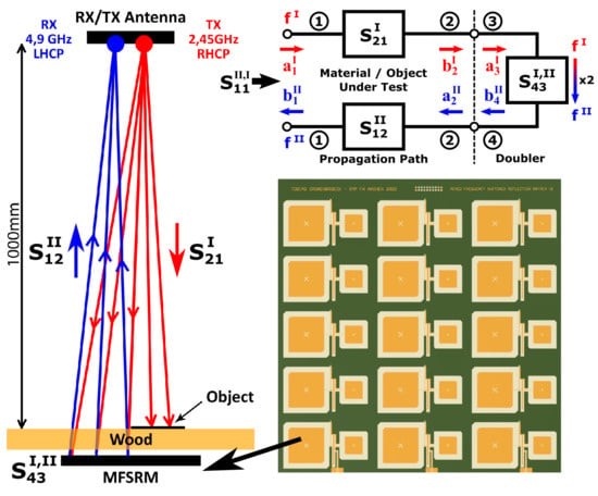
Figure 1 shows the typical scenario of an HR for a reference measurement without material under test (MUT) between the antennas. According to [
14,
24], the harmonic return signal power
at the interrogator’s receiving antenna feed point can be calculated using the HR equation by evaluating
using the nonlinear pseudo harmonic radar cross section (RCS)
of the tag, defined as
with
for the gain of the interrogator harmonic receiver antenna,
for gain of the interrogator’s fundamental frequency illumination signal antenna,
for the gain of the tag’s illumination signal reception antenna, and
for the gain of the tag’s harmonic re-transmission antenna. Furthermore,
and
denote the free-space wavelengths of the illumination and harmonic return signals, while
R denotes the slant range between the interrogator and the tag. Finally,
denotes the input power at the interrogator’s illumination signal transmit antenna feed point, while
is a proportionality factor which describes the specific harmonic conversion efficiency of the frequency doubler used in the HR tag. A graphical representation of all these key HR system variables is presented in [
18] and an extensive experimental validation of the validity of Equation (
1) can be found in [
18,
24].
When comparing Equation (
1) with the classical (monostatic) radar equation, two important observations fundamental to the optimization and design of harmonic radar systems can be made. The first is the different proportionality of the return signal strength for a given system and constant RCS target when the transmission power or range to target is varied—the HR return signal
for a standard primary radar system. Additionally, it is easily observed that all fundamental frequency signal path components up to the input of the tag’s frequency doubler show a square law dependency with regard to the harmonic return signal, which is caused by the nonlinear input power dependent transfer function of the doubler circuit.
An important metric for optimizing the nonlinear frequency doubler is the actual received power
at its input.
can be calculated by combining the normal one-way path loss formula to calculate the illumination field strength at the slant range
R and the effective antenna area of the fundamental frequency receiving antenna of the tag in the form of the HR radar equation
when omitting negligible loss contributors, such as the insertion loss of the transmission lines on the PCB.
The phase component
of the measured harmonic return signal phasor can be determined by following the progression of the signal phase through all system components, which is shown extensively in [
19,
24]. In this context, it is only important to know that the received harmonic signal phase can be calculated using
with
denoting the illumination signal’s angular frequency,
describing an arbitrary but repeatable phase offset, the phase propagation velocity
through the dispersion-less medium, and
R describing the mechanical slant range covered during propagation, when a memory-less power series model for the frequency doubler is assumed.
It is important to note for this application that the frequency doubling process results in an increased sensitivity of the propagation phase with regard to the propagation medium or material when compared with fundamental frequency SFCW radar. A similar observation can be made for the loss contributions of the material under test due to the square-law dependence of the return magnitude upon the received illumination signal power by the tag. Both observations combined lead to a greater sensitivity of such a system for small dielectric and loss variations in the material or object under test.
In reality, nonlinear frequency doublers are, however, far from ideal components and must be designed and optimized for a specific set of conditions relating to the measurement setup at hand. A longer discussion about the design of these components in the context of HR can be found in [
19]. For the scope of this article, it is sufficient to note that the use of HR leads to additional boundary conditions for the system, which are imposed by the transmission through a lossy medium between the HR interrogator and the tag. These conditions must be met for the validity of Equations (
1) and (
5). Ideally, the HR tag is operated in its well-defined square law transfer function region without saturation by the illumination signal, while still providing enough harmonic output power to obtain a good SNR at the receiver.
In order to describe the actual frequency converting nonlinear measurement in the HR setup, it is useful to describe the transfer functions using mixed frequency scattering parameters (MF-parameters), which are much easier to employ and understand than X-parameters in this context and are described in-depth in the text book [
25]. In keeping in-line with the definition of normal linear S-parameters, the measured frequency converting reflection parameter
measured by the system shown in
Figure 1 from the stimulus frequency
I to the harmonic response frequency
can be written as
, which relates the received harmonic complex power wave
at point D in
Figure 1 to the transmitted fundamental frequency power wave
at point A as measured by a VNA, formally described as
When this measurement is performed without a material or object under test, as shown in
Figure 1, the obtained result is the so-called reference measurement
and must be performed and stored for each HR tag element. This frequency converting reflection parameter can be further divided into distinct system contributions captured by this measurement, when mismatching between individual MF-parameters blocks is ignored and only the superposition of multiple reflection effects to the forward transmission is considered. This first order approximation is applicable and valid here due to the large free-space wave propagation losses.
Starting from the interrogator, the first relevant MF-parameter block is the linear forward propagation of the fundamental frequency stimulus signal through the medium to the input of the frequency doubler, which shall be denoted as
. The nonlinear, input power dependent MF-parameter of the doubler can be described by the parameter
, while the linear return path through the medium at the harmonic frequency is captured by
. A graphical representation of the HR signal flow is shown in
Figure 2. The complete reference measurement
can therefore be described using
Equation (
7) describes the HR transfer function for the reference measurement.
This reference result is used further on to normalize the measurement results obtained when a material or object under test is inserted into the pathway, which corresponds to the mixed-frequency equivalent of the reflection normalization procedure used in linear VNAs (see [
26]). This measurement implicitly contains the propagation properties of the channel at the two frequencies as well as the specific conversion behavior of the HR tag. Additionally, these data are also used to correct for systematic and repeatable phase offsets in the signal generation and receiver parts of the system (see [
19] for details).
An object- or material-under-test (MUT) shall have the scattering parameters
and
at the two frequencies I and II, which describe the superposition of all changes in transmission wave propagation caused by the material. When this material- or object-under-test is inserted into the propagation path, replacing a section of the free space reference measurement, and a measurement
is performed, a superposition of diffraction and refraction effects in addition to an observed change in phase velocity
and losses caused by the dielectric and magnetic properties of the material influencing the wave transmission through the material will occur. Since the material replaces an equivalent shaped section of free space contained in the reference measurement, it is necessary to de-embed the corresponding free-space section from the material properties, resulting in scattering parameters
and
, which only capture the relative change compared to an equivalent section of free-space propagation. The corresponding HR transfer function for the measurement including the MUT is therefore
The mechanical distance between the HR and the tag is unchanged compared to the reference measurement. The added material/object creates the observed additional attenuation and phase rotation and .
The nonlinear change of the transmission behavior of a frequency doubler
only influences the magnitude according to the following formulas:
when the doubler is operated in its square-law region where the memory-less power series approximation is applicable [
14,
18,
27].
The full normalized measurement with a material or object under test can therefore be described by
While the increased amplitude sensitivity of such a system is immediately obvious from Equation (
11), the increased phase sensitivity of the HR principle is not directly obvious and hidden in the formal definition of the phase between different frequencies in the MF-parameters, but is obvious when looking in the range information conveyed in the harmonic phase progression shown in Equation (
5):
While a normal transmission measurement system would only see a perceived increase in electrical length of
(
), a reflective normal radar system would see a perceived increase of
(
=
) due to the double transmission through the material, while a HR system sees a perceived path length increase of
due to the doubling of the instantaneous phase of
at the frequency doubler’s input and the return path performed at doubled stimulus frequency via
(see [
19] for derivation).
Equation (
11) can be used to calculate the expected response of different materials and objects over frequency with the results obtained by a mathematical model or 3D finite element method simulation. A database of such expected responses can then be used in addition to actual measurements to train an AI model for object or material recognition to classify the results of an actual unknown measurement. At the end of this paper, a traceable measurement in a performed in a closed, non-radiating, coaxial system is shown to prove the validity of Equation (11) and thus also Equation (9) in magnitude and phase.
3. Realization of the SIMO Harmonic Radar
The SIMO HR has one major difference from a standard SIMO radar. While the latter generally comprises a large number receiving antennas forming individual receiver channels, the new SIMO HR concept presented here only uses a single receiving antenna for the whole scene—the individual signal return and propagation path are formed using a number of inexpensive tags (transponders) which can be selectively sequentially activated to build the SIMO radar picture of the scene.
Therefore, the SIMO HR can be divided into the two distinct hardware modules: The HR radar front-end and the mixed frequency switched reflection matrix (short tag matrix or MFSRM). In the following, these two assemblies are presented and preliminary first measurements are shown.
3.1. Realization of the Harmonic Radar Frontend
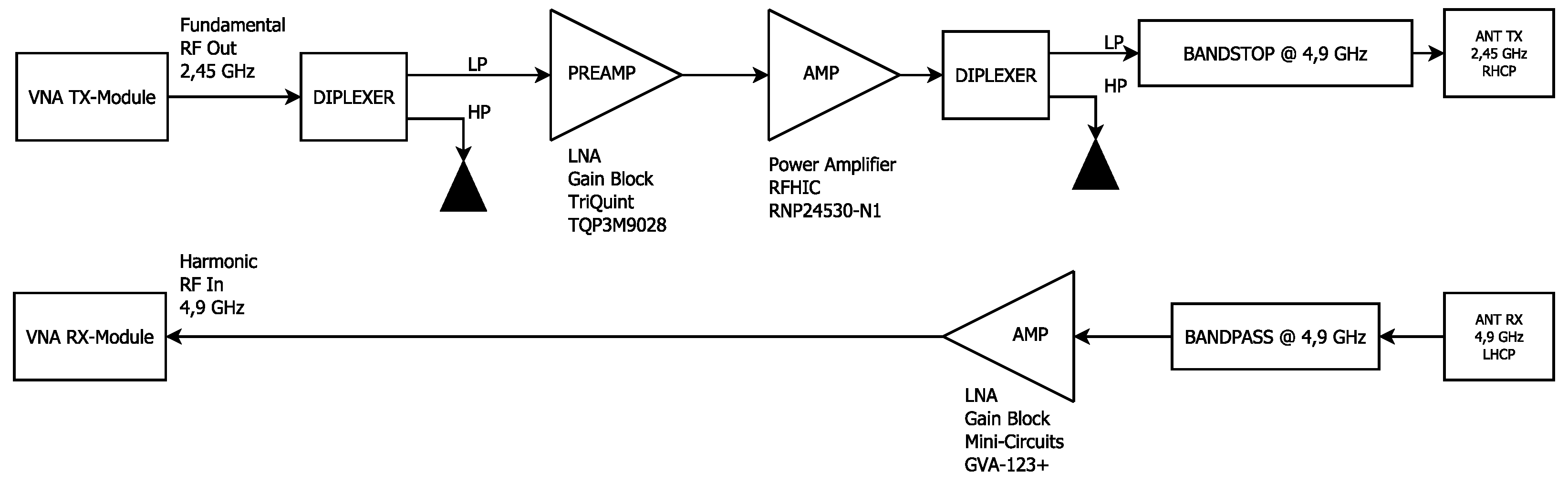
The radar front-end of the frequency-converting transfer function is based on the TX and RX VNA modules already cited and which are able to cover a frequency range of 275 to 6600 MHz. The schematic representation of this structure is shown in
Figure 3. The system design presented here follows the principles for highly linear HR interrogator design laid out in [
18,
19,
28].
The signal chain of the HR frontend starts with the generation of the stimulus illumination signal by the TX module of the VNA system. This signal is stabilized in its output power by a calibrated automatic level control loop and is repeatable in its phase relative to the reference clock of the system, even in fractional-N synthesis frequency hopping operation, which mitigates the need for an output signal measurement in the system as generally employed in VNAs (see [
18] for background and derivation).
In this setup, the TX module either generates a discrete set of consecutive sinusoidal signals of differing frequencies centered around 2.45 GHz (SFCW) or a configurable CW tone. This signal is subsequently low-pass filtered by a diplexer forming an absorptive low-pass filter to remove any residual harmonic content produced by the signal synthesis process and avoid the subsequent amplification of these residual interference products.
The filtered signal is then amplified by a linear driver gain block and a subsequent power amplifier to an output power of up to 33 dBm. Considerable output power back off (at least 7 dB) is employed to operate the PA in a linear region. Since even the most linear power amplifiers generally show a weak nonlinear behavior, the amplified output signal is then filtered again by an absorptive low-pass filter, which also helps to avoid inadvertent load-pulling on the PA by presenting a resistive termination for the second harmonic. Finally, the stimulus signal is then filtered again using a reflective 4.9 GHz band-stop filter with 60 dB suppression which ensures that any residual harmonics that occur are reduced to the absolute minimum before the illumination signal is radiated by the fundamental frequency antenna into the scene.
In the receiving path of the experimental setup, a reflective band-pass filter centered around the harmonic frequency of 4.9 GHz is used to suppress fundamental frequency break-through, which could lead to unwanted localized harmonic generation in the rest of the signal receiving chain, which especially includes the following MMIC gain block used to amplify the harmonic return signal for the mixed-frequency VNA receiver module. A picture of the assembled harmonic radar front-end electronics hardware setup is shown in
Figure 4.
The HR interrogator uses a custom planar dual-band patch antenna array for the TX (centered at 2.45 GHz, 4 elements) and the RX signal (centered at 4.9 GHz, 5 elements). Opposing circular polarizations (2.45 GHz RHCP, 4.9 GHz LHCP) were chosen to improve the isolation between RX/TX array elements and allow for a compact antenna layout, where the 4.9 GHz patch elements are nested between the larger 2.45 GHz patches. Besides the obvious reduction in overall size, this arrangement of the patch elements also reduces the signal loss introduced by diffraction and refraction of the waves by the MUT for a non or weakly dispersive MUT in a non-perpendicular surface orientation. This makes it easier to calculate MUT analyses and representations later on, without having to take possible interference into account. Patch antennas are very suitable for this application because they are very easy to mass-produce and have the appropriate directivity for whole scene illumination and reception in this setup.
The antenna was designed using a 4 layer PCB stack-up consisting of two Rogers RO4534 1.524 mm low-PIM substrate cores with an intermediate 0.2 mm center prepreg. The top layer contains the antenna elements, while the back layer is used for the matching, phase, and the power splitter/combiner networks. Both inner layers are used as RF ground planes. An organic silver surface finish was chosen to retain the very good PIM performance of the bare substrate, which allows this antenna to be used for HR for illumination signal input powers of up to 200 W. Individual highly linear P-SMP connectors ( @ 2 × 43 dBm) are used for connecting to the TX/RX chain. A realized antenna gain of approximately 11 dBi was achieved for both the TX and the RX antennas. The input return loss is better than 10 dB over the whole 2.45 GHz ISM band and its doubled harmonic counterpart at 4.9 GHz. Full width at half maximum (FWHM) beamwidths of 60° at 2.45 GHz and 35° at 4.9 GHz were realized. The antenna efficiency calculated by HFSS is above 83 % for both types.
A picture of the final realization of the HR front-end antenna is presented in
Figure 5.
3.2. Realization of the HR Tag Matrix
The development of the harmonic radar tag matrix was started with its basic building block—the HR tag cell. Due to economic reasons, a two-layer Isola Itera RF substrate with a thickness of 0.508 mm was chosen to realize the matrix. In a longer development process in Ansys HFSS to balance bandwidth, gain and return loss of the planar antennas on the thin substrate two RX/TX patch antennas for the tags were developed. The finally manufactured antenna visualized in
Figure 6 has the following dimensions:
RX antenna: length and width 32.1 mm, beveled corner 2 mm, slot length 5.6 mm and slot width 0.6 mm, TX antenna: length and width 16 mm, beveled corner 1 mm, slot length 2.3 mm and slot width 0.4 mm.
The corresponding matching values are −12 dB for both bands in the band center. The feed point impedances were chosen so that the antennas could be matched over the widest possible bandwidth.
The switchable frequency doubler, which also supports a tuning capability via its bias voltage, requires even more development effort than is reflected in its simple circuit topology shown in
Figure 7. This nonlinear microwave circuit was simulated and optimized with the help of the harmonic balance simulation function of the RF circuit simulator Keysight
ADS-Advanced Design System using the spice and scattering parameters provided of the components supplied by the manufacturer. Additional background information about the design and characterization of cooperative HR tags can be found in [
18,
19,
29,
30,
31]. In this design, a BAT15 Schottky diode from Infineon was used as the nonlinear element of the tag, while the BAR64 PIN diode from Infineon was used as an RF switch for the illumination signal at the nonlinear element’s input. A custom equivalent circuit model was fitted for the PIN diode from the available manufacturer data and the series inductances and pad capacities of the discrete components used were also taken into account. The antenna feed point impedance obtained by the simulation in HFSS were used as port impedance in the harmonic balance optimization process.
In order to optimize the tag in the harmonic balance simulation for operation in the square-law transfer function region, it is important to obtain an approximate figure of the available illumination signal input power at the doubler’s input, which can be calculated using classical link budget models. The path loss according to Friis transfer equation at 2 m distance from the tag reflection matrix is:
When a transmission of an illumination signal with a transmit power of +27 dBm = 500 mW EIRP, equivalent to +17 dBm at the TX antenna’s feedpoint at a frequency of 2.45 GHz is assumed, the input power to the doubler can be estimated with the transponder’s illumination signal receiving antenna gain of 6.9 dBi to be
which is certainly an absolute best case figure and can be used as the worst case scenario for avoiding harmonic compression effects in the doubler. In practice, this figure can be used as the criterion for the 1 dB harmonic compression point if the nonlinear element, as the matching network, the PIN diode switch, and the transmission lines will introduce at least 1…1.5 dB of insertion loss. The design of the matching network in combination with the harmonic balance simulation model of the diode was checked for this limit and optimized for maximum conversion gain and bandwidth at lower input powers, including a DC bias voltage sweep of the Schottky diode.
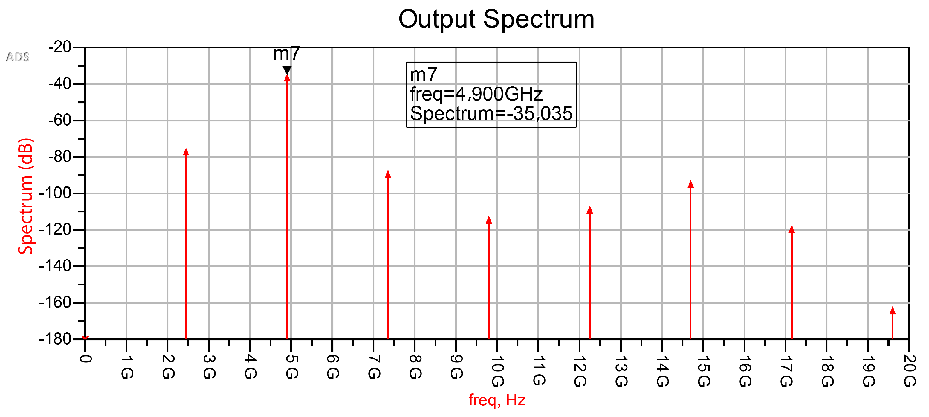
A typical harmonic balance simulation result of the complete circuit including higher harmonics is shown in
Figure 8 for a DC bias voltage of 0.5 V.
Due to the narrowband nature of the distributed element matching network, and higher order harmonics from 7 GHz upwards are substantially attenuated, no unwanted interference of systems operating in these higher frequency bands is to be expected, especially when the tuned bandpass response of the tag’s harmonic TX patch antenna is also taken into account.
The aforementioned HR tag cells can then be tessellated in one more dimension to form the mixed frequency switched reflection matrix. For our first experimental setup, the tags were placed in a 3-by-5 pattern to match the maximum space available in the standard RF prototype PCB manufacturing process of the contract manufacturer. The full switched harmonic radar tag matrix is shown in
Figure 9.
In the configuration shown, it is possible to measure 15 different complex transmission paths with this matrix without moving the MUT or any other mechanical movement of the system. For these measurements, it is guaranteed that the positions of the antennas are optimally maintained, which is very helpful for many evaluation procedures.
In order to control the individual HR tag cells of the matrix, a digital control unit was developed (
Figure 10), which consists of a STM32F4 microcontroller, four quad channel SPI DACs (MCP4728), 16 operational amplifiers (TLV274) for output voltage scaling and associated support circuitry. With this control unit, it is possible to set individual bias voltages for each cell element in the range of −3 V to +5 V in 12 bits of resolution by the control software of the system from a PC via USB serial interface. Additionally, a CAN bus interface is also supported for controlling the operation of the matrix at longer distances from the controlling PC.
Since the bias settings of each tag cell element can be individually controlled, a calibration routine for maximum conversion gain during the on-state and the minimal amount of harmonic return signal in the off-state can be run for each element, its values stored and later re-applied during actual measurements. This procedure helps to account for non-avoidable part to part variations in the assembly process of the PCB and for manufacturing variances present between each of the diodes used in the cells and is performed in situ to account for environmental effects.
The complete measurement setup is controlled by a custom application written in Python, which controls both the configuration and measurement taken by the VNA system as well as the operation of the mixed frequency switched reflection matrix.
4. First Measurements Performed with the SIMO HR Setup
For the first measurement using the SIMO HR setup presented here, the interrogator antenna was placed at distance of 1 m on a scaffold above a wooden table surface. The mixed frequency switched reflection matrix (see
Figure 9) was placed below the table surface and propped up using an empty shipping box at a distance of approximately 10 cm below the lower table surface.
A picture of this setup is presented in
Figure 11. The matrix cell bias optimization routine was executed, with the results shown in
Figure 12 and an initial reference measurement was performed to capture the undisturbed propagation paths to all individual cell elements of the matrix.
A small metal plate was then inserted into the propagation path on top of the table’s surface. Sequential measurements of the propagation paths to each cell element were then performed for different positions of the metal plate. A simple visualization of the measurement results was performed by plotting the change in magnitude for each propagation path normalized to the reference measurement as a change in color for a 3-by-5 pixel bitmap.
The setup and general location of the metal plate and the results for the two measurements are shown in
Figure 11 on the right and left of the laptop. The relative change in path magnitude is visualized in the color change from blue (equivalent to 1) to a more reddish color (representing values close to 0) in a color gradient. The position of the metal plate can easily be inferred from these plots.
The visualization results for a larger metal plate are shown in greater detail on the left side of
Figure 13, while the right side shows a visualization of the obstruction imposed by the metal plate upon the matrix as seen from the interrogator antenna’s beam boresight in a planar top-down projection during this measurement.
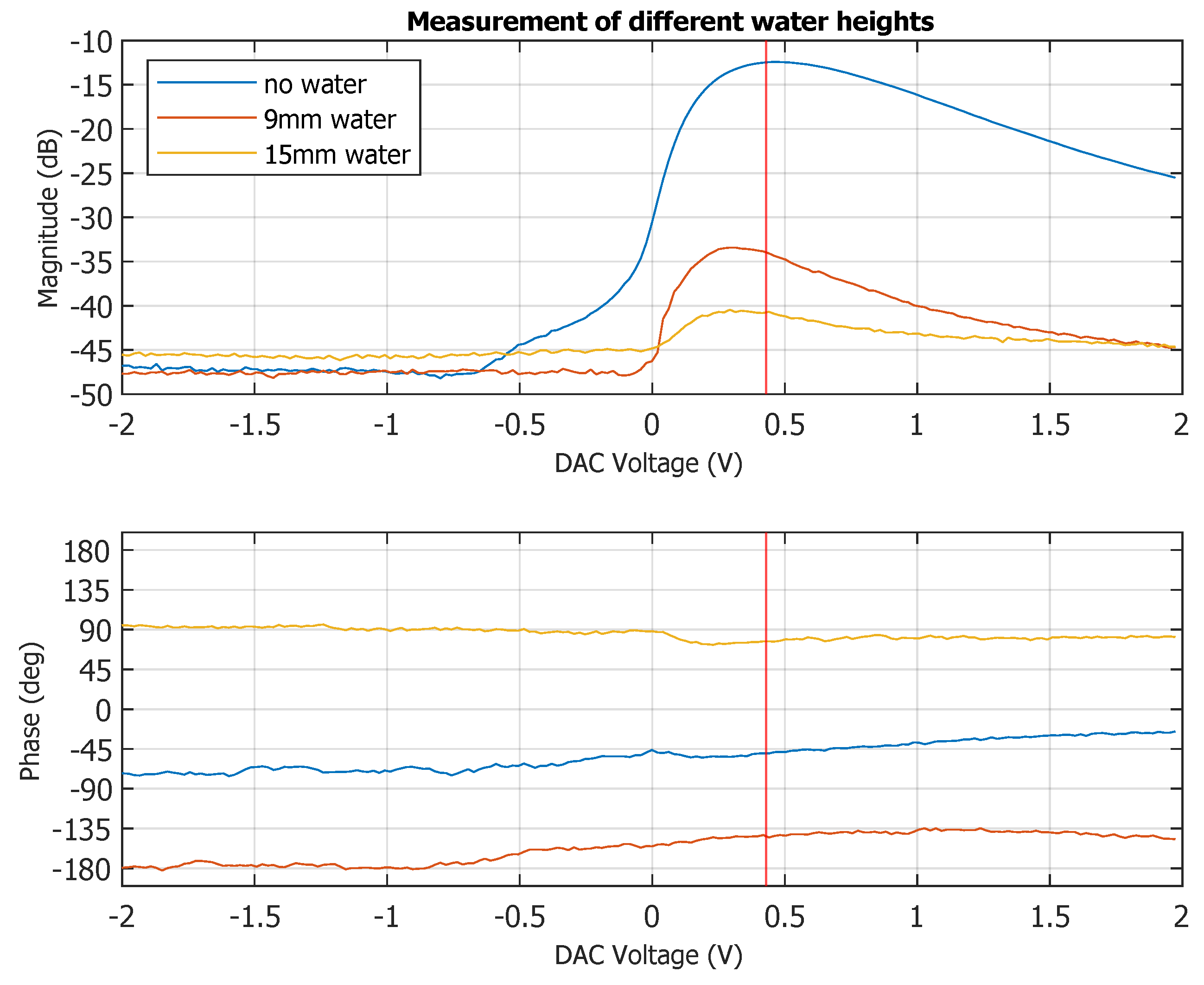
The final measurement results presented here are shown in
Figure 14 to demonstrate the propagation phase sensitivity of the system. For these measurements, only a single HR tag cell array was used in CW mode at 2.45 GHz, and a small plastic bowl was inserted into the propagation path (blue line in
Figure 14).
The bowl was then filled to a height of 9 mm with tap water (red line) and finally filled up to the height of 15 mm (yellow line) to avoid a phase rollover. The DC bias voltage of the cell element was varied during the measurement to demonstrate the dynamic range and phase variability over bias voltage of one HR-cell. Peak conversion gain occurred at a DC bias voltage of 0.45 V, and the plastic bowl and different water height can easily be discerned from another in the normalized measurement results relative to the undisturbed reference measurement (0 dB and 0°) of the HR tag cell.
The measurement was carried out at only one fixed frequency. These results reflect that very good results for the magnitude measurements are obtained with this setup over a dynamic range of more than 30 dB in transmission loss. The phase results, which are based purely on the time of flight, show almost constant values over the complete bias range for the doubler diode.
In a measurement for a material or object analysis, one uses the doubler diode at the bias voltage of 0.45 V and a frequency sweep.
5. Upcoming Measurements with the SIMO HR System and Outlook
The authors are currently in the process of developing and building an automated test setup to move materials and objects under test precisely and repeatable in one dimension through the electronically switched propagation paths of the system to facilitate the development of imaging generating harmonic SAR signal processing algorithms or to train neuronal networks for object recognition and/or feature extraction from the obtained data.
The mechanical scanning in one dimension was chosen to emulate a much larger mixed frequency switched reflection matrix for the time being until additional funding is acquired. While a 1D-cell line array would be sufficient in this setup, the electronic switching between three rows of lines reduces the measurement time by reducing the amount of precise mechanical movement needed to scan a given number of positions and/or propagation paths.
It is planned to put the first measurements performed in this setup on the web by the time this article is published. A description of the experimental setup, an explanation of the data format, and the links to the measurement data will be available at the link
https://www.researchgate.net/project/Mixed-frequency-S-parameter-measurements from August 2022. These measurements are intended for signal processing oriented scientists who want to perform MUT material analysis and/or MUT/object visualization using this new SIMO HR system without going through all the troubles associated with developing and building a SFCW HR system, as no commercial off the shelf turn-key solution systems are available.
The SIMO HR system shown here can also be employed in a multitude of configurations otherwise not feasible for transmission based radar and material analysis systems, as no RF cables are required on the far side of the MUT and no mechanical scanning of the radar antenna is necessary. An exemplary massive SIMO setup consisting of several mixed frequency switched reflection matrices oriented throughout a scene is shown in
Figure 15. When a sufficient amount of MFSRM units are positioned throughout the scene, a multitude of RF propagation effects such as diffraction, refraction, knife-edge diffraction reflection, and plane wave reflection can be used for feature extraction.
In larger radar scenes, it would also be feasible to use individual HR tag cells fitted with an independent power source and with a radio data link for switching control to perform complex measurement tasks, such as wall material composition, structure and moisture analysis radar [
32,
33,
34], and precise position monitoring of assets such as glacier movement or bridge vibration analysis [
35,
36] in harmonic CW doppler radar mode without impairment by clutter.
Furthermore, the cells used in this first implementation of the mixed frequency switch reflection matrix only employed as passive nonlinear element in its design even though a power supply is available—while suitable for short distances and lower GHz frequencies—this principle can also easily be extended to longer ranges by using cell design based upon an active low power frequency doubler based upon SiGe BJTs [
18] or other various active nonlinear elements (see the very good overview presented in [
37]) or even extended into the millimeter wave regions for much higher range resolution by using the method shown in [
38], which would even allow such applications as millimeter wave body scanners to use a massive MIMO setup.
6. Verification of the HR Transfer Function
In order to verify the HR transfer function in a free-space environment in a scientifically sound manner, a large anechoic measurement room is necessary to exclude the unknowns and uncertainties associated with multi-path propagation effects. Since this equipment and space is not readily available to the authors, the verification measurement was instead carried out in a coaxial line system, which allows a comparatively much higher amount of repeatability, lower uncertainty, and ease of traceability by allowing the independent fundamental and harmonic transfer function measurements to be performed by a VNA using a precision calibration kit.
For the verification measurement, the HR system presented and explained in [
19], which contains the same VNA modules as the SIMO device presented here, was used to build a harmonic reflectometer to perform the same normalized harmonic
reflection measurements as the system presented previously, although in a slightly different frequency range (2900…2940 MHz fundamental signal, 5800…5880 MHz harmonic signal) due to the required filters and diplexers, as well as the narrow-band power amplifier, for its intended application in the maritime S-band. A schematic block diagram of the setup is shown in
Figure 16 and an annotated picture of the verficiation setup is shown in
Figure 17.
A suitable coaxial harmonic reflection tag equivalent was constructed by combining a passive transmission doubler circuit based upon the HSMS-286F zero-bias Schottky diode (see [
19] for characterization and explanation) with a diplexer and a harmonic band reject filter for the fundamental frequency input of the doubler into a one-port nonlinear device.
A 40 dB coaxial attenuator is placed between the harmonic reflectometer and the surrogate harmonic radar tag at the normalization reference plane to fulfill three different important tasks: First, this attenuator acts as a stand-in for the free-space attenuation normally experienced by the stimulus and harmonic return signals. Second, this attenuator allows the operation of the doubler in its optimized square law transfer function region without the onset of harmonic compression at stimulus power levels below −21 dBm, despite the fairly high (+15 dBm) minimum output power signal provided by the setup. Finally, this attenuator also provides a good hardware source match at the reference plane to reduce the influence of matching errors without full (mathematical) system error correction to hold up the assumptions made when deriving the normalized HR transfer function shown in Equation (
11).
Four coaxial SMA attenenuators (see
Figure 17) with different nominal transmission attenuation values (3 dB, 6 dB, 10 dB and 20 dB), made by three different manufacturers in slightly varying form factors resulting in distinct transmission phases, were used as a well-defined coaxial replacement devices for an MUT. S-parameter measurements were obtained for all attenuators using a Rohde & Schwarz ZVA67 VNA in a frequency step-size of 1 MHz at an IF bandwidth of 100 Hz for all relevant frequency ranges. A Rosenberger precision 3.5 mm male/female calibration kit in combination with the unknown-thru calibration and correction procedure was used for full two-port S-parameter error correction and to account for the insertable mixed SMA connector gender (VNA port 1 male, port 2 female) of the attenuators with a correct position of the S-parameter reference plane. The acquired complex linear S-parameters (
and
) of all devices are shown in
Figure 18.
This setup used here illustrates that an HR can also be used as a vectorial measuring network analyzer, whereby the measured values contain the classical transfer function
, which in practice also corresponds to the reverse transfer function
due to reciprocity, several times and in two frequency ranges. For this coaxial verification measurement scenario, the following assumption is applied to the transfer functions of the reference measurements:
which leads to the position of the normalization reference plane for
as shown in
Figure 16 and
Figure 17. The nonlinear one-port element is assumed to obey the memory-less square law transfer function as explained during the derivation of Equation (
11) and to show an unknown but repeatable harmonic conversion
performance. This unknown offset is removed by storing the initial measurement of the nonlinear element without a device inserted into the reference plane and normalizing the subsequent measurements performed with devices-under-test (DUT) to this result (nonlinear reflection normalization).
It is important to note that, in contrast to the freespace formulation of Equation (
11), these devices here are completely inserted into the position of the reference plane; therefore, we can replace the designation MUTz with the designation MUT in Equation (
11), as no part of the setup present under the reference measurement conditions is replaced for the DUT measurements.
Therefore, the original Equation (
11) can be rewritten in the form of
which is the equivalent form for the insertable coaxial case of the original free-space reference measurement formulation of this equation and is used in the following to verify the validity of the original assumption. Both equations share the same the rough modeling of the doubler.
In order to carry out this verification, all four attenuators were measured with the best accuracy available to the authors with a correct definition of the connector insertion plane using an VNA. The results are shown in
Figure 18. An indication for the high measurement accuracy are the very small deviations for the magnitude values, which are less than 0.01 dB in the band up to 2940 MHz and less than 0.02 dB in the band from 5800 MHz. These linear S-parameter values were then used to calculate the expected results for
using Equation (
15) for all four devices.
Then, the HR measurement using the setup shown in
Figure 16 and
Figure 17 were carried out. The system was allowed to reach thermal equilibrium for a duration of 2 h before the measurements took place. In order to gain some statistical significance of the results, four distinct measurement runs containing all the devices were conducted sequentially. One sequence contains the following measurement: the initial reference measurement without a DUT that is stored for normalization of the data acquired during the run, a re-measurement of the reference configuration with normalization applied to check for drift and data validity, the measurement of the 3 dB, 6 dB, 10 dB, and 20 dB attenuators inserted into the reference plane and finally another re-measurement of the reference configuration, which is then used for the normalization of the following run. The results were calculated from the complex average of
measurements. This complex measurement sequence was carried out to minimize the influence of system drift upon the results. Additionally, the mean received scalar harmonic return power
in the harmonic return frequency band is also acquired for each measurement.
The results for
obtained by these measurements are shown in
Figure 19 (solid colored lines) in addition to calculated model values (dashed black line). It is important to note that the frequency axis only shows the harmonic return frequency for reasons of clarity, instead of the formally correct 2-tuple
associated with the mixed frequency S-parameter.
The measurement results obtained for the three lower value attenuators (3 dB, 6 dB, and 10 dB) show a very good signal-to-noise ratio and a good agreement with the data obtained by the simple square-law transfer function model of Equation (
15) applied to the one-port nonlinear element, especially considering that no systematic error correction was applied to the data obtained by the HR system and the limited repeatability of normal SMA connectors. In these measurements, the observed error of the HR data compared to the model is less than 1 dB in magnitude and less than 4° in phase. We believe these minor residual errors are due to a combination of different factors, mainly the idealization of the doubler but also due to the nonexistent systematic error correction (when compared to a VNA) and the limited connector repeatability in this setup. Based on this assumption, we consider the proof of the HR transfer function to be satisfied.
While the results of the the 20 dB attenuator measurement shown in
Figure 19 show a larger amount of error compared to the other results, the mean received scalar harmonic return power
values shown in
Table 1 serve to put these results into perspective and show the performance of this HR setup, since the harmonic return power values were only around −147 dBm for this DUT, which shows that the limited signal-to-noise ratio is the limiting factor here. Furthermore, the good results obtained in the
measurement can also be seen in the difference in scalar harmonic power levels between DUTs and good repeatability between runs for the four different DUTs in the values shown in
Table 1.


