Progress Guidance Representation for Robust Interactive Extraction of Buildings from Remotely Sensed Images

Abstract

Accurate building extraction from remotely sensed images is essential for topographic mapping, cadastral surveying and many other applications. Fully automatic segmentation methods still remain a great challenge due to the poor generalization ability and the inaccurate segmentation results. In this work, we are committed to robust click-based interactive building extraction in remote sensing imagery. We argue that stability is vital to an interactive segmentation system, and we observe that the distance of the newly added click to the boundaries of the previous segmentation mask contains progress guidance information of the interactive segmentation process. To promote the robustness of the interactive segmentation, we exploit this information with the previous segmentation mask, positive and negative clicks to form a progress guidance map, and feed it to a convolutional neural network (CNN) with the original RGB image, we name the network as PGR-Net. In addition, an adaptive zoom-in strategy and an iterative training scheme are proposed to further promote the stability of PGR-Net. Compared with the latest methods FCA and f-BRS, the proposed PGR-Net basically requires 1–2 fewer clicks to achieve the same segmentation results. Comprehensive experiments have demonstrated that the PGR-Net outperforms related state-of-the-art methods on five natural image datasets and three building datasets of remote sensing images.

1. Introduction

The extraction of buildings from remotely sensed images is essential for topographic mapping and urban planning. Although automatic building extraction methods have been investigated for decades, they are still difficult to achieve sufficient performance to meet the requirements for fully automated use. Conventional methods mainly exploit empirically designed features to recognize buildings, such as color, texture, and shadow, etc. Due to the limitation of hand-crafted features, these methods usually produce frustrating results in complex scenes. In recent years, with the development of deep learning techniques, building segmentation performance has been lifted a lot by various deep convolutional neural networks (DCNNs), such as U-Net [1], SegNet [2], DeepLabV3+ [3]. These networks take RGB images as input and directly output the probability map of buildings in the image. By learning from massive amounts of training samples, they can achieve performance far beyond conventional methods. However, these CNN-based automatic building extraction algorithms are suffering from poor generalization ability, which means a well-trained network can only make good predictions on images with a similar distribution of the training data. Furthermore, the acquirement of pixel-wised annotated data itself is time-consuming and expensive, and the accuracy of the segmentation results is also far from the requirement of actual use.

Under these circumstances, the study of interactive building extraction is of great value and importance. Fully-automatic extraction methods are characterized by the prior constraints, such as shape and appearance of the buildings, and the output results are automatically generated and presented in front of the users before further processing. The main difference between fully-automatic and semi-automatic building extraction methods is that the latter can accept human supervision as additional input to ensure the quality of the output results. A good interactive segmentation method is always aimed at reducing the user effort. Actually, there was a significant amount of research before the advent of deep learning techniques. An earlier well-known method is intelligent scissors [4], which focuses on the boundary property for object extraction. Afterward, a graph model-based interactive image segmentation algorithm was studied a significant amount. Boykov and Jolly [5] utilize scribbles to estimate the probability of the foreground/background of the target object. The task is formulated as a graph partition problem and solved by a min-cut/max-flow algorithm [6]. Veksler [7] integrates a star-convexity shape into a graph-cut segmentation, and Gulshan et al. [8] further improve the results with multiple stars and geodesics distances. Rother et al. [9] take the bounding box as input and utilize a Gaussian mixture model for foreground and background prediction. Yu et al. [10] use a Markov Random Field (MRF) to segment objects with loosely bounded boxes. In addition, Grady [11] uses the label of the seed firstly reached by a random walker to mark unlabeled pixels. Limited by the capacity of these hand-crafted features, the amount of user inputs are still required in complex scenarios, such as low contrast and poor illumination.

Recently, deep learning techniques have also been applied to interactive object extraction and achieved great success in the field of computer vision. Xu et al. [12] first propose a CNN-based model for interactive segmentation and devise a click simulation strategy for the training of the network. They transform the user-provided clicks into Euclidean distance maps and concatenate them with RGB images as the input to the network. This work is then extended and improved by many other works in different aspects. For example, Mahadevan et al. [13] introduce an iterative way to improve the heuristic sampling strategy during the training stage. Li et al. [14] select the optimal result among multiple diverse solutions to reduce the user efforts. Majumder and Yao [15] combine superpixels and class-independent object proposals with user-provided clicks to generate more informative guidance maps for the performance promotion of interactive segmentation systems. Jang and Kim [16] propose a backpropagating refinement scheme (BRS) to guarantee the correct prediction in user-annotated positions. Sofiiuk et al. [17] further propose a feature backpropagating refinement scheme (f-BRS) to alleviate the computational burden of the forward and backward pass. Lin et al. [18] consider that the first click contains location guidance of the main body of the target object and put forward a first click attention module to make better use of the first click.

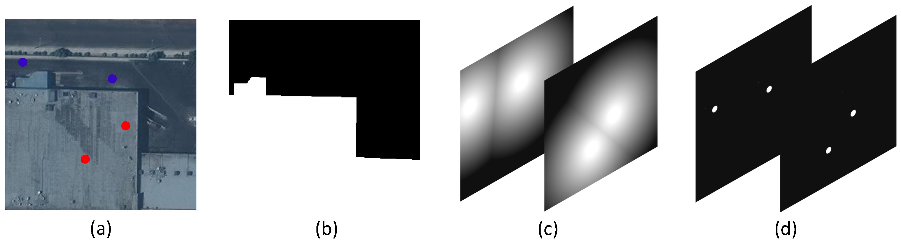
Generally speaking, user inputs are typically given as clicks [12,13,14,15,16,17,18,19], scribbles [5] and bounding boxes [9,10]. Compared with the other two modes of interactions, the click-based way is relatively simple and can reduce the burden of the annotators. In this work, we focus on the study of click-based interactive extraction of buildings. In this setting, users sequentially provide positive points on the foreground or negative points on the background to interact with the model until the segmented results are satisfied. To feed the interaction information to the CNN-based interactive segmentation model, an important issue is how to encode the user-provided clicks. 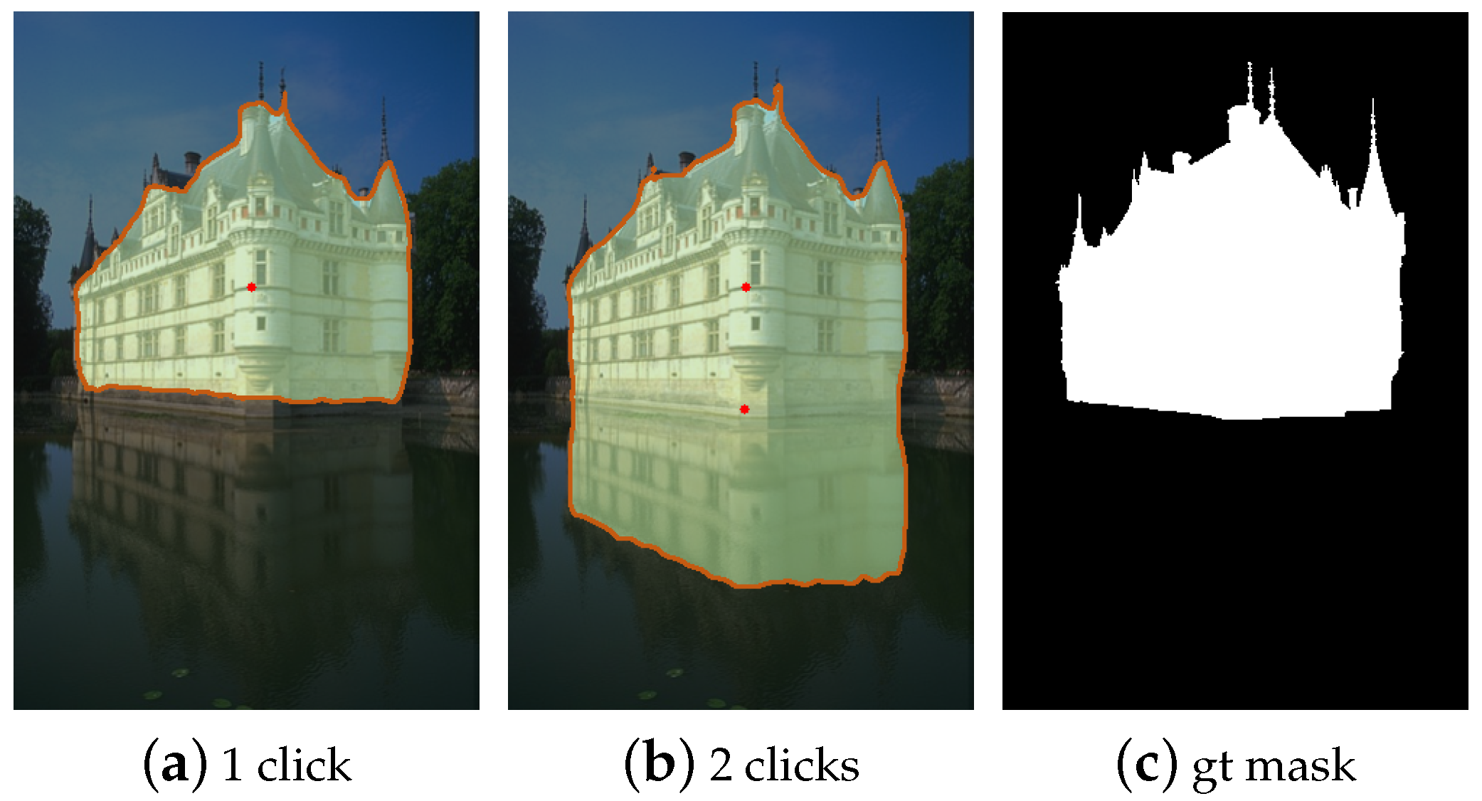Most of the existing methods follow [12] to simulate positive and negative clicks and transform them into a two-channel guidance map by Euclidean distance [12,14,16,17,19] or gaussian masks [18], and we utilize a satellite image in CrowdAI [20] dataset to demonstrate this in Figure 1. These two encoding methods are simple and straightforward representations of user-provided click points, which are convenient for the simulation of the training samples and the batch training of the network. In addition, they are also flexible in dealing with objects of multi-parts or weird shapes in natural scenes. However, such two-channel representations lack enough information to make an interactive segmentation network maintain good stability. In Figure 2, we present an image segmentation example of a baseline network in a natural scene that only utilizes guidance maps transformed from the user-provided clicks by Euclidean distance. We can see that the building is almost perfectly segmented after the first click. However, after the second click is added for further mask refinement, the segmentation result is severely degraded. It is because the predictions are independent at each step both in the training and inference stages. The guidance map treats all clicks independently, the network basically predicts the mask of the target object by the distribution of the positive and negative click points. Furthermore, the Gaussian masks of clicks or Euclidean distance maps are a kind of “weak” guidance, which is not conducive to the stability of mask refinement.

In our opinion, an interactive segmentation process is a coarse-to-fine process, which is carried out with two objectives, the fast estimation of the scale of the target object and the continuous refinement of the predicted masks. These two objectives conflict in the extent of the change to the previous segmentation mask. The former focuses on flexibility, and the latter emphasizes stability. A robust interactive segmentation system should progressively improve the segmentation mask with as little oscillation as possible because a false prediction will require additional clicks to revise. We argue that existing guidance maps are flexible representations for dealing with complex objects in natural scenes. However, compared with objects (multi-parts, elongated) in natural scenarios, buildings in overhead remote sensing images tend to have relatively regular shapes. For these “easy” buildings, the stability of the interactive segmentation process is critical to the improvement of performance. Motivated by the above circumstances, in this work, we focus on developing a robust interactive building extraction method based on CNN. To promote the stability of the interactive segmentation network, we firstly combine the previous segmentation map, which is considered as a kind of “strong” guidance, with existing distance-based guidance maps. In addition, we observe that annotators often tend to click around the center of the largest misclassified region. Thus, in most cases, the distance of the newly added click to the boundary of the previous segmentation mask can provide instructive progress information of the interactive segmentation process. This distance can be easily obtained during the inference stage, and we call this distance the indication distance. We make use of this distance and transform it into another guidance map to increase the stability of the interactive segmentation model. Moreover, we propose an adaptive zoom-in strategy and an iterative training strategy for further performance promotion of the algorithm. Comprehensive experiments show that our method is effective in both natural scenes and remote sensing images. Especially, compared with the latest state-of-the-art methods, FCA [18] and f-BRS [17], our approach basically requires 1–2 fewer clicks to achieve the same segmentation results on three building datasets of remote sensing images, which significantly reduces the workload of users. Furthermore, we propose an additional metric for the further evaluation of the robustness of the proposed interactive segmentation network, and the experimental results demonstrate that our approach yields better stability over other methods.

Our contributions can be summarized as follows:

• We analyze the benefits of a segmentation mask to improve the stability of network prediction, and we combine it with existing distance-based guidance maps to promote the performance of the interactive segmentation system.
• We also propose an adaptive zoom-in scheme during the inference phase, and we propose an iterative training strategy for the training of an interactive segmentation network.
• We achieve state-of-the-art performance on five widely used natural image datasets and three building datasets. In particular, our approach significantly reduces the user interactions in the interactive extraction of buildings. Comprehensive experiments demonstrate the good robustness of our algorithm.

The remainder of this article is arranged as follows: Section 2 describes details of the proposed method; the corresponding experimental assessment and discussion of the obtained results are shown in Section 3 and Section 4, respectively; Section 5 presents our concluding remarks.

2. Materials and Methods

In this section, we provide the details of the proposed algorithm for the interactive extraction of buildings in remote sensing images. Firstly, we introduce the datasets utilized in our study in Section 2.1. Then, we describe the detail of the proposed PGR-Net in Section 2.2. Finally, the implementation detail is presented in Section 2.3.

2.1. Datasets

A CNN-based interactive segmentation network is characterized by class-agnostic object extraction, which requires a dataset with diversity for the training to ensure the performance and generalization ability. In this study, in order to train the proposed PGR-Net, we follow [14,16,17] to adopt Semantic Boundaries Dataset (SBD [21]) as the training data and evaluate on five natural image datasets. Moreover, to verify the effectiveness of the proposed PGR-Net on buildings, we select three building datasets for detailed evaluation. The details of these datasets are described as follows.

2.1.1. Natural Image Dataset

We use Semantic Boundaries Dataset (SBD) to train our model, and test on five datasets to evaluate the performance of our algorithm, the details of utilized datasets are described as follows:

• SBD [21]: The dataset contains 8498 training images and 2820 test images. Following [16,17], we use the training set of this dataset to train our network, and the test set, which contains 6671 instances, is utilized for the evaluation of our algorithm.
• GrabCut [9]: The dataset consists of 50 images with a single object mask provided for each image. It is used as a common benchmark for most interactive segmentation algorithms.
• Berkeley [22]: The dataset contains 200 training images and 100 test images. It contains some challenging segmentation scenarios such as low contrast between the foreground and the background. We use 100 object masks on 96 test images as in [16] for the evaluation.
• DAVIS [23]: This is a benchmark dataset for video segmentation. It contains 50 videos with high-quality annotated masks. We sample the same 10% frames as [17,18] for the evaluation.
• MSCOCO [24]: This dataset is a large instance segmentation dataset, which contains 80 object categories. We sample 10 images per category to compose a test set of 800 images as in [17].

2.1.2. Building Dataset

We utilize three building segmentation datasets to validate the effectiveness of our algorithm; two of them are publicly available (AIRS [25], CrowdAI [20]) and the other is annotated by our team, named EVLabBuilding. The details of these datasets are as follows:

• AIRS [25]: This is a large-scale aerial imagery dataset for roof segmentation. It provides high-quality roof annotations for 7.5 cm resolution images. We crop the provided training images into $480\times 480$ image patches and select 3398 images for testing.
• CrowdAI [20]: This is a large dataset for the extraction of building footprints in satellite images. The dataset annotates buildings at the instance level, and each individual building is annotated in a polygon format according to MS COCO standards. All the images are $300\times 300$ pixels with a resolution of 0.3 m. We use the provided small subset of the validation set, which contains 1820 images, for testing.
• EVLabBuilding: It is a mixture dataset of aerial images of Guangzhou and Zhengzhou, China. It contains 40 images with resolutions ranging from 0.15 to 0.3 m. The buildings are annotated at the instance level by Earth Vision Lab, Wuhan University. We crop the images into $512\times 512$ pixels and finally produce 3669 patches for testing.

In Figure 3, we present some example images of each dataset. As it can be seen, images in the AIRS dataset are of high quality. The CrowdAI dataset contains many small buildings and the images are also blurry. The scenes in the EVLabBuilding dataset are usually very messy, which is very challenging for the extraction of buildings. It is noted that for each image, we randomly choose one building instance from it for evaluation. For a fair comparison, we determined these instances in advance and used them for the evaluation of all algorithms.

Furthermore, achieving the same IoU score is often more difficult for small objects. In order to facilitate a more detailed analysis of the algorithm, we further divide the test set into three subcategories according to the size of the buildings. Specifically, we classify the buildings into Small Buildings ($\alpha \le {20}^2$), Medium Buildings (${20}^2\le \alpha \le {60}^2$) and Large Buildings ($\alpha >{60}^2$); here $\alpha$ denotes the area of the building (number of pixels). The details of the divided subcategories of each dataset are listed in

Table 1. Details of divided subcategories of AIRS, CrowdAI and EVLabBuilding datasets.

Dataset	Small	Medium	Large	All
AIRS	222	672	2504	3398
CrowdAI	388	966	466	1820
EVLabBuilding	348	1064	2257	3669

.

2.2. Methods

In this section, we first introduce the preparatory concept indication distance of the proposed PGR-Net in Section 2.2.1. Afterward, we present the input and the structure of the PGR-Net in Section 2.2.2. In Section 2.2.3, we show how to simulate the training samples for the training of the PGR-Net. Finally, the adaptive zoom-in technique and the iterative training strategy are described in Section 2.2.4 and Section 2.2.5, respectively.

2.2.1. Indication Distance

Our approach is based on the assumption that annotators are always accustomed to clicking around the center of the main misclassified regions for the segmentation mask refinement. Under this circumstance, we notice that the minimal distance of the newly added click to the boundary of the previous mask has a good indication of the segmentation progress, and here we refer to this distance as the indication distance. In Figure 4, we show an example to illustrate our point. We can easily infer that the indication distance is large when the previous segmentation mask is far from the ground truth, otherwise this distance is relatively small.

In some special cases, as shown in Figure 5, for objects with holes, multi-parts or elongated parts, indication distance sometimes may provide misleading guidance. Fortunately, the impact of these issues is negligible with a large amount of data training. These scenarios can be covered in the training set by data simulation and iterative training, which will be discussed in Section 2.2.3 and Section 2.2.5, respectively. In addition, to further reduce the impact of these circumstances, we force the indication distance to keep decreasing during the inference phase. Specifically, at each step, the current indication distance is determined by $curdist=min(lastdist,curdist)$, where $lastdist$ denotes the indication distance of the previous step.

2.2.2. Guidance Representation and Network Structure

With humans in the loop, the interactive segmentation can be viewed as a sequential decision problem, which contains abundant information, such as previous segmentation results, history clicks, and newly added clicks, etc. There are various ways to encode the user input. Most of the existing methods follow [12] to simulate positive and negative clicks and transform them into guidance maps by Euclidean distance [14,16,17,19] or Gaussian masks [18]. Such representation treats all clicks indiscriminately. Furthermore, we argue that the click maps or their corresponding transformed distance-based maps are “weak” guidances, which is not conducive to the stability of the network prediction. Considering that the previous segmentation mask can provide “strong” guidance of the existence of target objects, we experimentally combine it with the newly added click map to feed into an interactive segmentation network and found out that the output tends to be consistent in the final detail refinement stage. We consider it is because this guidance representation lacks information of history clicks.

Therefore, we combine all the information mentioned above to form a new guidance representation and feed them to the interactive segmentation network. Figure 6 shows an overview of our method. Our guidance map consists of four parts, positive and negative click maps, newly added click map and the previous segmentation map. We utilize the same transform strategy for all click-related map generation. Given a set of click points $p_{ij}\in A$, where $(i,j)$ is the point location, then for any point $p_{mn}$ in the 2D matrix with the same sized input image, its corresponding value $V\left(p_{mn}A\right)$ is computed as follows:

$$V\left(p_{mn}A\right)=\underset{\forall p_{ij}\in A}{min}\sqrt{{(i-m)}^2+{(j-n)}^2}$$

(1)

The 2D matrix is normalized into [0, 1] as the final guidance map.

$$V^{\prime }\left(p_{mn}A\right)=1-{\displaystyle \frac{min(V\left(p_{mn}A\right),d)}{d}}$$

(2)

For positive and negative click maps, we chose d as 10. Notably, we set d to 30 for the first click, which means there is only one positive click and no other negative clicks. The newly added click map is a single channel, d is set equal to its corresponding indication distance, and we set the matrix negative if the newly added click falls into the background.

In this paper, we do not focus on the network architecture design. In Figure 7, we present the network structure of the PGR-Net. We follow [26] and utilize a modified ResNet [27] architecture as our backbone, in which the stride of the last two layers are reduced to one and dilation convolution is employed, which helps to increase the resolution of the output feature and maintain the receptive field of the network at the same time. In Appendix A, we present the detailed structure of the backbone network. Afterward, we add skip-connections in the encoder to aggregate both the low-level and high-level features. Specifically, the features “conv1”, “res1”, “res2” and “res4” of the backbone network are converted into a 128-d feature by a $3\times 3$ convolutional layer, respectively. Subsequently, we upsample these features to the same resolution as “conv1” and concatenate these 128-d features to obtain a 512-d feature. Finally, we employ a PSP module [28] to obtain the prediction mask.

2.2.3. Simulating User Input

To simulate the previous segmentation mask, we follow [29] to generate perturbed segmentations with various shapes. Specifically, we subsample the contour of the ground-truth mask, and then perform multiple random dilation and erosion operations. After the simulation of the previous segmentation mask, we set the center point of the largest error region as the newly added click for corresponding guidance map generation.

For the simulation of positive and negative clicks, we adopt the sampling strategy proposed in [12]. The numbers of positive and negative clicks are determined randomly within [1, 10] and [0, 10], respectively. The click points are generated in sequence, and for the positive clicks, the new point is sampled in the foreground with at least $d_p^1$ pixels from the object boundary and $d_p^2$ pixels from existing points. For negative clicks, the new point is sampled in the background with $d_n^1\sim d_n^2$ pixels away from the object boundaries and $d_n^3$ pixels away from existing click points. We set $d_p^1=5$, $d_p^2=10$, $d_n^1=5$, $d_n^2=40$, and $d_n^3$ is set to 10.

Notably, the training samples are generated based on object instances, each object in the image is individually selected for training sample simulation. For each object, multiple training samples can be obtained by simulating different clicks and masks. In Figure 8, we present two examples of simulated training samples.

2.2.4. Adaptive Zoom-In

Different from fully automatic image segmentation, in the interactive setting, objects are gradually refined and extracted in an iterative and interactive manner. Thus, cropping is a simple and effective manner for the detail refinement of the segmentation mask, especially for the small objects. Sofiiuk et al. [17] call this technique zoom-in and firstly introduce it to the interactive segmentation system.

The premise of applying zoom-in is that the network has predicted an approximate mask of the ground truth, inappropriate use may lead to degradation of the network output. Therefore, the evaluation of the quality of the current segmentation mask is of great importance. Sofiiuk et al. [17] notice that the first three clicks are sufficient for the network to obtain a rough mask of the target object. They empirically crop the image according to the bounding box of the predicted mask after the third click. Such a heuristic method is not applicable to all situations. In our work, the indication distance can accurately reflect the quality of the segmentation mask, and we exploit it to apply zoom-in prediction adaptively. Specifically, when the indication distance is smaller than a certain threshold $T$, we crop an image according to the bounding box of the predicted object mask to obtain a zoom-in region, which will be resized to a target size $S$ and fed into the network for the next prediction. For the bounding box, we extend $C$ pixels along the longest side direction to preserve the context, and the shortest side will be extended adaptively to form a square box. Notably, we only apply zoom-in for small objects, which means the size of the extended bounding box should be smaller than $S$, and the bounding box will be adjusted if a user provides a click outside the box.

By our adaptive zoom-in technique, the network is able to handle objects of different scales in a more flexible manner, which is helpful to promote the stability of the network and reduce the user interactions. We will further discuss the superiority of our adaptive zoom-in technique over the empirical way in Section 4.2.

2.2.5. Iterative Training Strategy

To facilitate the batch training of deep learning networks, most click-based interactive segmentation methods adopt a random sampling strategy for generating clicks. Such a sample generation strategy does not consider the sequential relationship of user-provided clicks during the inference stage. Thus, the iterative training strategy, where new clicks are added based on the prediction errors of the network during training, is often utilized to boost the performance, and this strategy is widely used and proved to be effective for interactive segmentation algorithms.

In our algorithm, there is always a gap between the simulated perturbed segmentations and the network predictions. Furthermore, our positive and negative clicks are also randomly generated. For the above considerations, we propose an iterative training strategy for the training of our model. Specifically, we incorporate the adaptive zoom-in technique into the standard iterative training procedure proposed by [13], and an example of the corresponding iterative training process is shown in Figure 9. The simulated guidance maps are fed into the network to obtain a prediction. Based on the misclassified region, we use the same clicking strategy as the inference stage to provide a new click. If the indication distance of the newly added click is smaller than $T$, then we crop and resize the patch of the object to form new training data, and the related guidance maps will be transformed accordingly. In this way, we align the network training to the actual usage. This can also be regarded as a kind of data augmentation, which is helpful for improving the performance of the algorithm.

2.3. Implementation Details

We formulate the interactive segmentation problem as a binary segmentation task and use binary cross entropy loss for the network training. We use zero initialization for the extra channels of the first convolutional layer. We utilize Semantic Boundaries Dataset (SBD [21]) to train our model. The input images are randomly cropped into $384\times 384$ pixels, and the dataset is augmented by a horizontal flip. We take ResNet-101 pre-trained on ImageNet [30] as the backbone. The batch size is 4. We set an initial learning rate of 3 × 10${}^{-5}$ for ResNet and 3 × 10${}^{-4}$ for other parts. We use the Adam [31] optimizer to train our network for 32 epochs. The learning rate decreases by a factor of 10 after every 10 epochs. The network is implemented in the PyTorch framework and trained on a single NVIDIA GeForce RTX 2080Ti GPU.

For the automatic evaluation of our algorithm, we use the same clicking strategy as the previous works [16,17,18] to simulate user interaction. At each step, we obtain a segmentation mask predicted by the network, and then the new click will be added at the center of the largest misclassified region. The first click is added in the same way, with the network prediction being regarded as zero. For the zoom-in prediction, we choose the indication distance threshold $T$ as 20 pixels, and the extended size $C$ is 30, the target size $S$ is set to 480.

For the evaluation of related algorithms, the mask intersection over union (mask IoU) is adopted as a basic metric in our experiments. First, we follow [16,18] to utilize two performance measures to compare our algorithm with other state-of-the-art methods. One is the NoC metric, which indicates the average number of clicks to reach a certain IoU threshold on each sample of a dataset. We set the maximum number of clicks to 20 for each sample. The other is the plot of the mean IoU score according to the number of clicks. We also compute the area under curve (AuC) for each method, with each area normalized into [0, 1].

3. Experimental Results

Segmentation performance and generalization ability are two important indexes for the evaluation of an interactive segmentation method. To assess the effectiveness of the proposed PGR-Net, we devise two groups of experiments on natural scene images and high-resolution remote sensing datasets, respectively. We first follow References [14,16,17] to evaluate our algorithm on five widely used natural image datasets to demonstrate the generalization ability of PGR-Net. Afterward, to facilitate the detailed analysis of our method on the interactive extraction of buildings, we analyze and compare our algorithm with the latest state-of-the-art methods FCA [18] and f-BRS [17] on three building datasets of remote sensing images. In addition, we conduct detailed ablation experiments to verify the effectiveness of each component, and analyze the stability of our algorithm.

3.1. Evaluation on Natural Image Dataset

We compare our approach with other existing methods, including GrabCut (GC) [5], geodesic matting (GM) [32], random walk (RW) [11], Euclidean star convexity (ESC) [8], geodesic star convexity (GSC) [8], Growcut (GRC), deep object selection (DOS) [12], regional image segmentation (RIS) [19], latent diversity based segmentation (LD) [14], backpropagating refinement scheme (BRS) [16], content aware multi-level guidance (CMG) [15], feature backpropagating refinement scheme (f-BRS) [17], and first click attention network (FCA) [18].

Figure 10 illustrates the IoU scores of each method on the different number of clicks. In general, deep-learning-based methods (solid lines) have better performance than traditional interactive segmentation algorithms (dashed lines) in all datasets. The curve of our method is smooth, and we achieve the highest AuC scores across all five datasets, which means our algorithm has a better performance. Specifically, the curves of our method have obvious advantages on SBD and COCO datasets, and for the DAVIS, due to its difficulty, the curves of each algorithm are relatively close. In

Table 2. Comparison of the number of clicks (NoC) required to reach IoU 0.85 (NoC@85) and 0.9 (NoC@90) on GrabCut, Berkeley, DAVIS, SBD and COCO datasets. The best and the second-best results are boldfaced and underlined, respectively.

Method	GrabCut		Berkeley	DAVIS	SBD		COCO
	NoC@85	NoC@90	NoC@90	NoC@90	NoC@85	NoC@90	NoC@85	NoC@90
GC [5]	7.98	10.00	14.22	17.41	13.6	15.96	15.23	17.61
GM [32]	13.32	14.57	15.96	19.50	15.36	17.60	16.91	19.63
RW [11]	11.36	13.77	14.02	18.31	12.22	15.04	13.62	16.74
ESC [8]	7.24	9.20	12.11	17.70	12.21	14.86	14.04	16.98
GSC [8]	7.10	9.12	12.57	17.52	12.69	15.31	14.39	16.89
DOS [12]	5.08	6.08	8.65	12.58	9.22	12.80	9.07	13.55
RIS [19]	-	5.00	6.03	-	-	-	-	-
LD [14]	3.20	4.79	-	9.57	7.41	10.78	7.86	12.45
BRS [16]	2.60	3.60	5.08	8.24	6.59	9.78	-	-
CMG [15]	-	3.58	5.60	-	-	-	5.92	-
FCA [18]	1.82	2.08	3.92	7.57	-	-	3.64	5.31
f-BRS [17]	2.30	2.72	4.57	7.41	4.81	7.73	4.11	5.91
Ours	1.99	2.26	3.66	7.05	3.70	5.67	3.25	4.26

, we report the NoC results on five datasets. We achieve the best performance on four of them. As it can be seen, our algorithm requires fewer number of clicks to reach the same IoU score. Note that we do not utilize complicated architecture design. However, the improvement of performance is significant, which demonstrates the effectiveness of our algorithm.

3.2. Evaluation on Remote Sensing Dataset

In Section 3.1, we conduct a detailed comparison and analysis of related interactive segmentation algorithms, including traditional and deep-learning-based. In this section, we select the most recent state-of-the-art methods (FCA [18] and f-BRS [17]) for the comparison.

In Figure 11, we present the IoU scores of each algorithm under a different number of clicks on the three datasets. Compared with the other two methods, our algorithm achieves the highest AuC scores in all the three datasets. Concretely, the advantages of our method on AIRS and EVLabBuilding datasets are huge and significant, and on the CrowdAI dataset, the performance of the algorithms are close and worse; we consider that this is because there are many small buildings on the CrowdAI dataset. Basically, it only takes 3–4 clicks for our algorithm to achieve good results. In

Table 3. Comparison of the number of clicks (NoC) required to reach IoU 0.85 (NoC@85) and 0.9 (NoC@90) on the AIRS dataset.

Method	Small		Median		Large		All
	NoC@85	NoC@90	NoC@85	NoC@90	NoC@85	NoC@90	NoC@85	NoC@90
f-BRS [17]	13.17	16.52	5.69	9.38	4.88	7.22	5.58	8.25
FCA [18]	16.62	18.83	5.05	8.51	3.26	4.80	4.48	6.45
Ours	15.94	17.45	4.27	7.05	2.57	3.33	3.78	4.99

,

Table 4. Comparison of the number of clicks (NoC) required to reach IoU 0.85 (NoC@85) and 0.9 (NoC@90) on the CrowdAI dataset.

Method	Small		Median		Large		All
	NoC@85	NoC@90	NoC@85	NoC@90	NoC@85	NoC@90	NoC@85	NoC@90
f-BRS [17]	13.54	16.97	9.20	13.93	9.02	13.54	10.08	14.48
FCA [18]	14.48	17.98	6.34	10.26	5.50	8.76	7.86	11.52
Ours	13.61	16.39	5.16	8.33	4.47	6.63	6.78	9.61

and

Table 5. Comparison of the number of clicks (NoC) required to reach IoU 0.85 (NoC@85) and 0.9 (NoC@90) on the EVLabBuilding dataset.

Method	Small		Median		Large		All
	NoC@85	NoC@90	NoC@85	NoC@90	NoC@85	NoC@90	NoC@85	NoC@90
f-BRS [17]	14.82	17.80	5.88	9.67	5.98	8.37	6.79	9.64
FCA [18]	18.22	19.72	6.19	11.06	4.53	6.55	6.31	9.11
Ours	10.98	13.64	3.67	5.25	3.73	4.65	4.40	5.68

, we report the quantitative NoC results of each algorithm on AIRS, CrowdAI and EVLabBuilding datasets, respectively. In fact, NoC results of small buildings ($20\times 20$) do not make much sense because it is always difficult for such small objects to reach 0.9 IoU. Nevertheless, our algorithm still performs significantly better than other methods in the NoC metric. For medium and large buildings, our algorithm basically only requires 1–2 fewer NoC than other methods to achieve the same IoU results, in some cases, it can reach 4–5 or more. Compared with the results of Table 2 in natural scenes, our results on buildings have more obvious advantages. We consider it is due to the better stability of our algorithm, and this advantage will be more prominent in “easy” buildings, of which we will make a further analysis in Section 3.4. In Figure 12, we also present some visualized comparisons of each algorithm on the three datasets.

3.3. Ablation Study

To further evaluate the efficacy of each component in our algorithm, we conduct an ablation study on Berkeley, COCO and EVLabBuilding datasets. We take the network that only uses the positive and negative clicks as input as the baseline, and we gradually add each component proposed in this paper for validation. In

Table 6. Ablation study of the proposed method on Berkeley, COCO and EVLabBuilding datasets. BS: baseline; AZI: adaptive zoom-in technique; Iter: iterative training strategy; Seg: previous segmentation mask and the newly added click map.

Settings	Berkeley	COCO		EVLabBuilding
	NoC@90	NoC@85	NoC@90	NoC@85	NoC@90
#1: BS	5.26	5.03	7.10	7.85	10.85
#2: BS + AZI	4.60	4.54	6.31	7.13	9.50
#3: BS + AZI + Iter	4.51	3.60	4.83	4.92	6.82
#4: BS + AZI + Iter + Seg	3.66	3.25	4.26	4.40	5.68

, we report the mean number of click (NoC) results of different settings. Overall, the iterative training (No.3) and segmentation guidance map (No.4) have brought significant performance improvement. By utilizing iterative training, the performance on the COCO dataset is improved with 0.94 and 1.48 alleviating of NoC; and for the EVLabBuilding dataset, the NoC value has been significantly reduced by 2.21 and 2.68. However, the improvement effect on the Berkeley dataset is very slight. We infer that it is because the iterative training and the data augmentation in it help the network to deal with some small or easy objects. However, for objects with complex shapes in the Berkeley dataset, the effect of improvement is limited. On the other hand, we consider that the previous segmentation mask can promote the stability of the mask refinement, which has more advantages in the detail refinement of complex objects. Thus, by adding the previous segmentation mask, the NoC on the Berkeley dataset is reduced from 4.51 to 3.66. We will compare the stability of No.3 and No.4 settings in Section 3.4 to further verify this point.

3.4. Stability Analysis

For the evaluation of the stability of interactive image segmentation algorithms, we use the frequency of “bad” clicks and the average IoU reduction caused by these “bad” clicks as a metric. The “bad” clicks here refer to clicks that cause the segmentation IoU to fall after being added to the network. Specifically, when calculating the NoC metric, we also count the frequency of “bad” clicks before the segmentation result reaches a certain IoU to evaluate the robustness of the interactive segmentation system. We compare our algorithm with f-BRS and FCA on the AIRS dataset. From the curves in Figure 10 and Figure 11, we can see that the IoU is basically saturated after reaching 90% for all methods. Thus, here we set the target IoU to 90% for a more reasonable evaluation, and the comparison results are shown in

Table 7. Comparison of the ratio of “bad” clicks and its corresponding average IoU reduction on the AIRS dataset. #ACs: number of all clicks; #BCs: number of bad clicks.

Method	#ACs	#BCs	Ratio	IoU Drop (avg.)
f-BRS [17]	28034	6132	21.87%	11.83%
FCA [18]	21925	3720	16.97%	7.46%
Ours−	21646	4386	20.26%	11.65%
Ours	16952	1499	8.84%	3.13%

. Our algorithm yields the lowest ratio of “bad” clicks, which means our algorithm is less prone to produce degraded results. Furthermore, the average IoU reduction of our method is 3.13%, and we consider it as a normal fluctuation during the final refinement stage of the segmentation masks. “Ours−” denotes the No.3 setting in Table 6, and from this, we can see the importance of the previous segmentation mask and the newly added click map for improving the stability of the network. The stability of FCA-Net is better than that of the f-BRS, which is because the first click attention module is helpful to promote the stability of the network prediction. Furthermore, we notice that the average IoU drop of f-BRS is 11.83%, which means that each “bad” click will cause a drop in IoU of 0.12. From this, we can infer that the results of f-BRS fluctuate sharply.

In Figure 13, we present a visualized interactive segmentation process of f-BRS, FCA and our algorithm on a test case of the AIRS dataset to further demonstrate the stability of our algorithm. We show the segmentation mask of each algorithm after each click is added before the IoU reaches 0.9. It only takes 4 clicks for our method to reach 0.9 IoU. In addition, our algorithm can continuously improve the segmentation results, while the segmentation masks of f-BRS (7th click) and FCA-Net (7th and 11th click) are easily degraded, which is harmful to the interactive segmentation system.

4. Discussion

4.1. Building Extraction Analysis

From the results in Table 2, Table 3, Table 4 and Table 5, we can see that our method surpasses FCA [18] and f-BRS [17] on both building and natural image datasets. Specifically, the advantage of our method is more obvious in dealing with buildings. We attribute this to the good stability of PGR-Net, which is essential for the interactive extraction of buildings. If an interactive segmentation algorithm is not stable, it will take a significant amount of clicks to extract even a very simple object. From the last row of Figure 12, we can see that for an easy building, f-BRS [17] takes 5 clicks to reach 0.9 IoU. This is because in the process of object extraction, the algorithm has been correcting the wrong prediction given by itself. We have provided an example in Figure 13 to demonstrate this point, and this is in line with our analysis in Section 1.

4.2. Adaptive Zoom-In

To demonstrate the superiority of our proposed adaptive zoom-in technique, we compare it with heuristic zoom-in strategies on Berkeley, DAVIS and EVLabBuilding datasets. We consider that the images in these datasets have different size, which is very suitable for such validation. Here we follow [17] to apply zoom-in prediction after 1, 3 and 5 clicks, and these three settings are denoted as “#1”, “#3” and “#5”, respectively. We compute and compare the NoC required for each setting to reach 0.9 IoU (NoC@90), and the results are reported in

Table 8. Comparison of the different zoom-in settings on Berkeley, DAVIS and EVLabBuilding datasets.

Setting	#1	#3	#5	Adaptive
Berkeley(NoC@90)	3.93	4.02	4.18	3.66
DAVIS(NoC@90)	7.29	7.18	7.22	7.05
EVLabBuilding(NoC@90)	5.64	5.79	6.11	5.68

. For the empirical zoom-in strategies, we can see that “#1” is the best on Berkeley and EVLabBuilding datasets. However, on the DAVIS dataset, “#3” performs best. This indicates a single empirical setting does not always achieve optimal performance in the face of different scenarios. On the contrary, our adaptive zoom-in strategy can always achieve good performance on all of the datasets.

4.3. Clicking Strategy

To analyze the impact of the clicking strategy to our algorithm, we analyze the IoU score according to the number of clicks on the Berkeley dataset with three different clicking strategies, and the related results are shown in Figure 14. In strategy 1, we use the center of the largest error region (point p) as the new click. In clicking strategy 2, we first compute the minimum distance of point p to the boundary, denoted as d, and then we randomly select clicks from the error region within $0.5d$ from point p. In strategy 3, we randomly select clicks in the largest error region. We can see that strategy 2 has a similar performance to strategy 1. However, when we randomly select clicks by using strategy 3, the performance of the network is degraded to some degree. It is because the indication distance will provide misleading guidance in this situation. To sum up, our algorithm can perform well when users provide clicks around the center of the misclassified region. However, when users click near the boundary of the mislabeled region, the performance will decrease to a certain extent. Overall, by referring to the results of other similar methods [13], we believe such performance degradation is normal and acceptable. In Section 4.4, we will further verify our algorithm by human study.

4.4. Interaction with Human Annotators

Our algorithm is based on the assumption that the annotators are accustomed to click around the center of the largest error region. Notably, we just utilize this information roughly to obtain the progress information of the interactive segmentation process, and we do not require the annotators to follow this strategy strictly. To further validate the robustness of the proposed algorithm, we conduct a small experiment with real human annotators in the loop. Based on the proposed interactive segmentation model, we develop a tiny annotation tool for the evaluation. Taking into account the workload of the annotators, we asked two human subjects to annotate the objects in the GrabCut dataset (50 images). Notably, we only explained how to use this tool, and the annotators do not know the details of the algorithm behind it. For each object, the corresponding ground-truth image is presented, and the annotators can provide clicks according to their preferences. Once the IoU score reaches 0.9, the tool will give a prompt, which also means the annotators have completed the annotation of this object. In

Table 9. Real human experiments on the GrabCut dataset.

	NoC@85	NoC@90
Automatic	1.99	2.26
Annotator#1	1.78	2.52
Annotator#2	1.80	2.56

, we compare the NoC results of different annotators with an automatic clicking strategy. NoC@85 and NoC@90 denote the NoC required to reach IoU 0.85 and 0.90, respectively. In general, the results are very close. An interesting finding is that the NoC@85 results of human annotators are generally better than the results of the automatic clicking strategy, while for NoC@90, the situation is the opposite. This is because in the automatic clicking strategy, clicks are determined by calculating the maximum distance of the misclassified area, and sometimes these clicks are not the “real” center of the object, which can degrade the performance of the segmentation results; thus, it takes more clicks to achieve IoU 0.85 (NoC@85). As for NoC@90, the reason is that for small objects, it is sometimes difficult for human annotators to provide further clicks because the result is already pretty good, it just does not reach 0.9 IoU.

5. Conclusions

In this work, we analyze the difference of objects in natural scenes and buildings in remote sensing images and realize that the stability is critical to an interactive segmentation system, especially for “easy” buildings. Focusing on the promotion of the robustness of the interactive segmentation, we utilize the distance of newly added clicks to the boundary of the previous segmentation mask as an indication of the interactive segmentation progress, and this information is employed with the previous segmentation mask and positive and negative clicks to form a progress guidance map. This progress guidance map is then fed into a CNN with the original RGB image. Furthermore, we propose an iterative training strategy for the training of the network. Moreover, we adopt an adaptive zoom-in technique during the inference stage for further performance promotion. Abundant experimental results show that our algorithm has good robustness and superiority. In particular, compared with the latest state-of-the-art methods, FCA [18] and f-BRS [17], the proposed PGR-Net basically requires 1-2 fewer clicks to achieve the same segmentation results on the three building datasets. Currently, our method is utilized for the extraction of building instances. In future research, we will try to improve our method for the interactive extraction of region objects.

References

1. Ronneberger, O.; Fischer, P.; Brox, T. U-Net: Convolutional Networks for Biomedical Image Segmentation. In Lecture Notes in Computer Science, Proceedings of the Medical Image Computing and Computer-Assisted Intervention—MICCAI 2015—18th International Conference, Munich, Germany, 5–9 October 2015; Proceedings, Part III; Springer: Berlin/Heidelberg, Germany, 2015; Volume 9351, pp. 234–241. [Google Scholar] [CrossRef] [Green Version]
2. Badrinarayanan, V.; Handa, A.; Cipolla, R. Segnet: A deep convolutional encoder-decoder architecture for robust semantic pixel-wise labelling. arXiv 2015, arXiv:1505.07293. [Google Scholar]
3. Chen, L.C.; Zhu, Y.; Papandreou, G.; Schroff, F.; Adam, H. Encoder-decoder with atrous separable convolution for semantic image segmentation. In Proceedings of the European Conference on Computer Vision (ECCV), Munich, Germany, 8–14 September 2018; pp. 801–818. [Google Scholar]
4. Mortensen, E.N.; Barrett, W.A. Intelligent scissors for image composition. In Proceedings of the 22nd Annual Conference on Computer Graphics and Interactive Techniques, SIGGRAPH 1995, Los Angeles, CA, USA, 6–11 August 1995; Mair, S.G., Cook, R., Eds.; ACM: New York, NY, USA, 1995; pp. 191–198. [Google Scholar] [CrossRef] [Green Version]
5. Boykov, Y.; Jolly, M. Interactive Graph Cuts for Optimal Boundary and Region Segmentation of Objects in N-D Images. In Proceedings of the Eighth International Conference On Computer Vision (ICCV-01), Vancouver, BC, Canada, 7–14 July 2001; Volume 1, pp. 105–112. [Google Scholar] [CrossRef]
6. Boykov, Y.; Kolmogorov, V. An experimental comparison of min-cut/max-flow algorithms for energy minimization in vision. IEEE Trans. Pattern Anal. Mach. Intell. 2004, 26, 1124–1137. [Google Scholar] [CrossRef] [PubMed] [Green Version]
7. Veksler, O. Star Shape Prior for Graph-Cut Image Segmentation. In Lecture Notes in Computer Science, Proceedings of the Computer Vision—ECCV 2008, 10th European Conference on Computer Vision, Marseille, France, 12–18 October 2008; Proceedings, Part III; Forsyth, D.A., Torr, P.H.S., Zisserman, A., Eds.; Springer: Berlin/Heidelberg, Germany, 2008; Volume 5304, pp. 454–467. [Google Scholar] [CrossRef]
8. Gulshan, V.; Rother, C.; Criminisi, A.; Blake, A.; Zisserman, A. Geodesic star convexity for interactive image segmentation. In Proceedings of the Twenty-Third IEEE Conference on Computer Vision and Pattern Recognition, CVPR 2010, San Francisco, CA, USA, 13–18 June 2010; pp. 3129–3136. [Google Scholar] [CrossRef]
9. Rother, C.; Kolmogorov, V.; Blake, A. “GrabCut”: Interactive foreground extraction using iterated graph cuts. ACM Trans. Graph. 2004, 23, 309–314. [Google Scholar] [CrossRef]
10. Yu, H.; Zhou, Y.; Qian, H.; Xian, M.; Wang, S. Loosecut: Interactive image segmentation with loosely bounded boxes. In Proceedings of the 2017 IEEE International Conference on Image Processing, ICIP 2017, Beijing, China, 17–20 September 2017; pp. 3335–3339. [Google Scholar] [CrossRef] [Green Version]
11. Grady, L. Random walks for image segmentation. IEEE Trans. Pattern Anal. Mach. Intell. 2006, 28, 1768–1783. [Google Scholar] [CrossRef] [PubMed] [Green Version]
12. Xu, N.; Price, B.; Cohen, S.; Yang, J.; Huang, T.S. Deep interactive object selection. In Proceedings of the IEEE Conference on Computer Vision and Pattern Recognition, Las Vegas, NV, USA, 27–30 June 2016; pp. 373–381. [Google Scholar]
13. Mahadevan, S.; Voigtlaender, P.; Leibe, B. Iteratively Trained Interactive Segmentation. In Proceedings of the British Machine Vision Conference 2018, BMVC 2018, Newcastle, UK, 3–6 September 2018; BMVA Press: Durham, UK, 2018; p. 212. [Google Scholar]
14. Li, Z.; Chen, Q.; Koltun, V. Interactive Image Segmentation with Latent Diversity. In Proceedings of the 2018 IEEE/CVF Conference on Computer Vision and Pattern Recognition (CVPR), Salt Lake City, UT, USA, 18–23 June 2018. [Google Scholar]
15. Majumder, S.; Yao, A. Content-Aware Multi-Level Guidance for Interactive Instance Segmentation. In Proceedings of the 2019 IEEE/CVF Conference on Computer Vision and Pattern Recognition (CVPR), Long Beach, CA, USA, 15–20 June 2019. [Google Scholar]
16. Jang, W.D.; Kim, C.S. Interactive Image Segmentation via Backpropagating Refinement Scheme. In Proceedings of the 2019 IEEE/CVF Conference on Computer Vision and Pattern Recognition (CVPR), Long Beach, CA, USA, 15–20 June 2019. [Google Scholar]
17. Sofiiuk, K.; Petrov, I.; Barinova, O.; Konushin, A. F-brs: Rethinking backpropagating refinement for interactive segmentation. In Proceedings of the IEEE/CVF Conference on Computer Vision and Pattern Recognition, Seattle, WA, USA, 14–19 June 2020; pp. 8623–8632. [Google Scholar]
18. Lin, Z.; Zhang, Z.; Chen, L.Z.; Cheng, M.M.; Lu, S.P. Interactive Image Segmentation With First Click Attention. In Proceedings of the 2020 IEEE/CVF Conference on Computer Vision and Pattern Recognition (CVPR), Seattle, WA, USA, 14–19 June 2020. [Google Scholar]
19. Liew, J.H.; Wei, Y.; Xiong, W.; Ong, S.H.; Feng, J. Regional Interactive Image Segmentation Networks. In Proceedings of the 2017 IEEE International Conference on Computer Vision (ICCV), Venice, Italy, 22–29 October 2017. [Google Scholar]
20. Mohanty, S.P. CrowdAI Dataset. Available online: https://www.crowdai.org/challenges/mapping-challenge/dataset_files (accessed on 12 June 2018).
21. Hariharan, B.; Arbelaez, P.; Bourdev, L.D.; Maji, S.; Malik, J. Semantic Contours from Inverse Detectors. In Proceedings of the International Conference on Computer Vision, Washington, DC, USA, 6–13 November 2011. [Google Scholar]
22. Mcguinness, K.; O’Connor, N.E. A comparative evaluation of interactive segmentation algorithms. Pattern Recognit. 2010, 43, 434–444. [Google Scholar] [CrossRef] [Green Version]
23. Perazzi, F.; Pont-Tuset, J.; McWilliams, B.; Gool, L.V.; Gross, M.H.; Sorkine-Hornung, A. A Benchmark Dataset and Evaluation Methodology for Video Object Segmentation. In Proceedings of the 2016 IEEE Conference on Computer Vision and Pattern Recognition, CVPR 2016, Las Vegas, NV, USA, 27–30 June 2016; pp. 724–732. [Google Scholar] [CrossRef]
24. Lin, T.; Maire, M.; Belongie, S.J.; Hays, J.; Perona, P.; Ramanan, D.; Dollár, P.; Zitnick, C.L. Microsoft COCO: Common Objects in Context. In Lecture Notes in Computer Science, Proceedings of the Computer Vision—ECCV 2014—13th European Conference, Zurich, Switzerland, 6–12 September 2014; Part V; Fleet, D.J., Pajdla, T., Schiele, B., Tuytelaars, T., Eds.; Springer: Berlin/Heidelberg, Germany, 2014; Volume 8693, pp. 740–755. [Google Scholar] [CrossRef] [Green Version]
25. Chen, Q.; Wang, L.; Wu, Y.; Wu, G.; Guo, Z.; Waslander, S.L. Aerial Imagery for Roof Segmentation: A Large-Scale Dataset towards Automatic Mapping of Buildings. ISPRS J. Photogramm. Remote Sens. 2019, 147, 42–55. [Google Scholar] [CrossRef] [Green Version]
26. Chen, L.; Papandreou, G.; Kokkinos, I.; Murphy, K.; Yuille, A.L. DeepLab: Semantic Image Segmentation with Deep Convolutional Nets, Atrous Convolution, and Fully Connected CRFs. IEEE Trans. Pattern Anal. Mach. Intell. 2018, 40, 834–848. [Google Scholar] [CrossRef] [PubMed]
27. He, K.; Zhang, X.; Ren, S.; Sun, J. Deep residual learning for image recognition. In Proceedings of the IEEE Conference on Computer Vision and Pattern Recognition, Las Vegas, NV, USA, 27–30 June 2016; pp. 770–778. [Google Scholar]
28. Zhao, H.; Shi, J.; Qi, X.; Wang, X.; Jia, J. Pyramid Scene Parsing Network. In Proceedings of the 2017 IEEE Conference on Computer Vision and Pattern Recognition, CVPR 2017, Honolulu, HI, USA, 21–26 July 2017; pp. 6230–6239. [Google Scholar] [CrossRef] [Green Version]
29. Cheng, H.K.; Chung, J.; Tai, Y.; Tang, C. CascadePSP: Toward Class-Agnostic and Very High-Resolution Segmentation via Global and Local Refinement. In Proceedings of the 2020 IEEE/CVF Conference on Computer Vision and Pattern Recognition, CVPR 2020, Seattle, WA, USA, 13–19 June 2020; pp. 8887–8896. [Google Scholar] [CrossRef]
30. Deng, J.; Dong, W.; Socher, R.; Li, L.J.; Li, K.; Fei-Fei, L. Imagenet: A large-scale hierarchical image database. In Proceedings of the 2009 IEEE Conference on Computer Vision and Pattern Recognition, Miami, FL, USA, 20–25 June 2009; pp. 248–255. [Google Scholar]
31. Kingma, D.P.; Ba, J. Adam: A method for stochastic optimization. arXiv 2014, arXiv:1412.6980. [Google Scholar]
32. Bai, X.; Sapiro, G. Geodesic Matting: A Framework for Fast Interactive Image and Video Segmentation and Matting. Int. J. Comput. Vis. 2009, 82, 113–132. [Google Scholar] [CrossRef]
Figure 1. (a) Original image and corresponding positive and negative clicks. (b) The gt mask, (c) guidance maps transformed by Euclidean distance transform. (d) guidance maps transformed by Gaussians.
Remotesensing 13 05111 g001
Figure 2. A failure case of existing methods that utilize guidance maps transformed from the user-provided clicks by Euclidean distance.
Remotesensing 13 05111 g002
Figure 3. Example images in AIRS, CrowdAI and EVLabBuilding datasets.
Remotesensing 13 05111 g003
Figure 4. Illustration of indication distance. For poorly segmented results, the indication distance of the newly added click is large; otherwise, it is relatively small.
Remotesensing 13 05111 g004
Figure 5. Some special cases of indication distance, such as objects with holes or multi-parts.
Remotesensing 13 05111 g005
Figure 6. Overview of our method. The input to the network consists of the RGB image, the previous segmentation mask, the newly added click map (single channel), and the positive and negative click maps.
Remotesensing 13 05111 g006
Figure 7. Architecture of our network.
Remotesensing 13 05111 g007
Figure 8. Two examples of simulated training samples.
Remotesensing 13 05111 g008
Figure 9. An example of training data generation by using the adaptive zoom-in technique during the iterative training process.
Remotesensing 13 05111 g009
Figure 10. Comparison of the average IoU scores according to the number of clicks (NoC) on GrabCut, Berkeley, SBD, DAVIS and COCO datasets. The legend contains AuC scores for each algorithm.
Remotesensing 13 05111 g010
Figure 11. Comparison of the average IoU scores according to the number of clicks (NoC) on AIRS, CrowdAI and EVLabBuilding datasets. The legend contains AuC scores for each algorithm.
Remotesensing 13 05111 g011
Figure 12. Visualized comparison of different methods on EVLabBuilding, AIRS and datasets. Red for positive clicks and blue for negative clicks.
Remotesensing 13 05111 g012
Figure 13. Visualized comparison of the segmentation process of f-BRS, FCA-Net and our algorithm on a test case of AIRS dataset. Red for positive clicks and blue for negative clicks.
Remotesensing 13 05111 g013
Figure 14. IoU scores according to the number of clicks of different clicking strategies.
Remotesensing 13 05111 g014