An Elevation Ambiguity Resolution Method Based on Segmentation and Reorganization of TomoSAR Point Cloud in 3D Mountain Reconstruction

Abstract

Tomographic Synthetic Aperture Radar (TomoSAR) is a breakthrough of the traditional SAR, which has the three-dimentional (3D) observation ability of layover scenes such as buildings and high mountains. As an advanced system, the airborne array TomoSAR can effectively avoid temporal de-correlation caused by long revisit time, which has great application in high-precision mountain surveying and mapping. The 3D reconstruction using TomoSAR has mainly focused on low targets, while there are few literatures on 3D mountain reconstruction. Due to the layover phenomenon, surveying in high mountain areas remains a difficult task. Consequently, it is meaningful to carry out the research on 3D mountain reconstruction using the airborne array TomoSAR. However, the original TomoSAR mountain point cloud faces the problem of elevation ambiguity. Furthermore, for mountains with complex terrain, the points located in different elevation periods may intersect. This phenomenon increases the difficulty of solving the problem. In this paper, a novel elevation ambiguity resolution method is proposed. First, Density-Based Spatial Clustering of Applications with Noise (DBSCAN) and Gaussian Mixture Model (GMM) are combined for point cloud segmentation. The former ensures coarse segmentation based on density, and the latter allows fine segmentation of the abnormal categories caused by intersection. Subsequently, the segmentation results are reorganized in the elevation direction to reconstruct all possible point clouds. Finally, the real point cloud can be extracted automatically under the constraints of the boundary and elevation continuity. The performance of the proposed method is demonstrated by simulations and experiments. Based on the airborne array TomoSAR experiment in Leshan City, Sichuan Province, China in 2019, the 3D model of the surveyed mountain is presented. Moreover, three kinds of external data are applied to fully verify the validity of this method.

1. Introduction

Tomographic Synthetic Aperture Radar (TomoSAR) achieves the elevation resolution of layover targets through multi-angle observation of the same observation scene. TomoSAR has become an advanced data collection tool for three-dimentional (3D) applications such as topographic surveying, urban surveillance, biomass estimation, cultural heritage assets, and monitoring of slow-moving landslides [1,2,3,4,5].

In 1995, the TomoSAR 3D imaging technology was demonstrated for the first time, which was of great significance in promoting the development of TomoSAR [6]. In 2006, Fornaro et al. provided the first validation of spaceborne long-term SAR tomography. Specially, the 3D imaging results from European Remote Sensing 1 and 2 (ERS-1 and ERS-2) satellites over the urban area of Napoli were presented [7]. Later, the high-resolution spaceborne SAR systems such as TerraSAR-X [8] and Cosmo-Skymed [9] were launched. With the acquisition of high-resolution TomoSAR data, there are many achievements regarding TomoSAR 3D reconstruction. TomoSAR 3D reconstruction mainly consists of two steps, including point cloud generation and point cloud processing. For the former, the mainstream methods are based on Compressive Sensing (CS). For the latter, the method of the human-made buildings has been hot research. Initially, most of methods based on the hypothesis of polyhedral building structure were demonstrated [10,11,12]. Considering the more complex buildings containing curved structures, methods for curved structures are required. Zhu et al. proposed a method suitable for the buildings with rectangular footprints and curved footprints [13]. In this method, the façade points are clustered into individual facades by K-means, and then the segmented plane or curved surface are further modeled and merged. Subsequently, Shahzad et al. proposed a robust reconstruction method for larger areas [14]. In this method, three-step automatic clustering (TSAC) is proposed to segment the building facades [15]. This method integrates the advantages of Density-Based Spatial Clustering of Applications with Noise (DBSCAN) and Mean Shift (MS).

Although the TomoSAR technologies have been well developed, there are several shortcomings in the spaceborne TomoSAR. First, due to the long revisit time, the spaceborne TomoSAR suffers from the problem of temporal decorrelation, especially for mountains with many distributed targets [16]. Second, the satellites only work on the ascending and descending orbits, which is not conducive to adjusting the observation trajectory [13]. Third, the spaceborne TomoSAR is inflexible and cannot respond quickly to the observation needs of a specific region. The airborne array TomoSAR can well address these problems by arranging the antenna array in the cross-track direction. The array TomoSAR system allows the acquisition of high-precision data for 3D mountain reconstruction [17,18]. The National Key Laboratory of Microwave Imaging Technology, Aerospace Information Research Institute, Chinese Academy of Sciences (AIRCAS), has developed the first airborne array TomoSAR system in China. In 2015 and 2019, two experiments based on this system were successfully conducted over both urban areas and mountain areas. Furthermore, a series of TomoSAR point cloud processing methods have been proposed and validated by the airborne array TomoSAR data. In 2017, Gaussian Mixture Model (GMM) was applied for TomoSAR 3D point cloud processing [19]. The GMM fully considers the distribution feature, and allows classification based on probability [20]. In 2019, Zhou et al. proposed an automatic method using neural networks to regularize the 3D building structures [21]. In 2020, Jiao et al. demonstrated the 3D reconstruction framework of buildings [22]. Moreover, driven by this advanced single-pass mode, the multiple scattering of TomoSAR building point cloud has been interpreted and applied to high precision 3D reconstruction [23,24].

However, there are few literatures on TomoSAR 3D mountain reconstruction. The 3D mountain model is relevant in many fields, such as global mapping, disaster assessment, and disaster relief. Due to the layover phenomenon, mapping in high mountain areas remains a difficult task. Motivated by these chances and needs, 3D mountain reconstruction based on the airborne array TomoSAR is meaningful. The mountain point cloud can be obtained by referring to the mainstream CS-based methods. When the elevation span of the scene is larger than the ambiguous elevation of the TomoSAR system, the restricted isometry property (RIP) criterion is not satisfied. The original point cloud is aliased in the elevation direction [25]. For low targets such as buildings, the elevation span of the scene can be known in advance. Therefore, the problem of elevation ambiguity can be solved by encrypting the baseline at the system level [26]. Notwithstanding, the mountainous terrain is highly undulating. It is difficult to know the elevation span in advance. It is a challenge to solve the problem of elevation ambiguity at the system level. In addition, there is a trade-off between the ambiguous elevation and the elevation resolution. Even if the ambiguous elevation meets the requirements that no elevation ambiguity occurs in the original point cloud, the elevation resolution may be reduced. Limited by the system parameters and the characteristics of the scene, the TomoSAR mountain point cloud has the problem of elevation ambiguity.

Due to elevation ambiguity, none of the existing TomoSAR point cloud processing methods can be directly applied to TomoSAR mountain point cloud processing. To overcome the problem, an elevation ambiguity resolution method is proposed in this paper. The main purpose of elevation ambiguity resolution is to move the points to the correct elevation position. Obviously, it is not optimal to estimate the elevation ambiguity number point by point. Inspired by the processing methods of buildings, segmentation can improve the efficiency of elevation ambiguity resolution by converting the point processing to category processing. Consequently, segmentation and reorganization are the two steps of the proposed method. Notably, due to the common influence of elevation ambiguity and layover, the original point cloud may be corrupted by intersection, which will increase the difficulty of segmentation. In the first step, the difficulty of segmentation can be well addressed by using DBSCAN and GMM jointly. In the reorganization step, the segmentation results are rearranged in the elevation direction by elevation extension and combination, and the real point cloud is further automatically extracted by geometric constraints. The main contributions are as follows:

(1)

A robust segmentation method combing DBSCAN and GMM is proposed. Compared with the traditional segmentation methods, the proposed method provides better segmentation of the TomoSAR mountain point cloud with intersection.

(2)

Motivated by segmentation, an ingenious reorganization method is given. Through elevation extension and combination, reorganization allows to construct all possible results of elevation ambiguity resolution instead of estimating the elevation ambiguity number point by point.

(3)

By analyzing the distribution law of TomoSAR point cloud, geometric constraints are given to ensure the automatic extraction of the real point cloud. If geometric constraints are not used, the processor needs to interpret and judge one by one from all the reorganization results.

This paper is organized as follows. Section 2 briefly introduces our airborne array TomoSAR system. Section 3 analyzes the difficulties in solving the elevation ambiguity problem. Furthermore, the distribution law of TomoSAR point cloud is demonstrated. In Section 4, the proposed method for elevation ambiguity resolution is introduced in detail. In Section 5, the processing results for both simulated data and real data are presented and quantitatively analyzed. As a comparison, the results of traditional methods are given. Besides, the 3D reconstruction results of airborne array TomoSAR are evaluated in detail on three kinds of external data, i.e., the optical image, AW3D30 DSM, and 1:10,000 DEM. Conclusions are given in Section 6.

2. Array TomoSAR System

Because of the problem of temporal decorrelation caused by long revisit time, the traditional TomoSAR systems with repeat-pass cannot obtain a well-focused point cloud in the elevation direction, especially for mountains. The first domestic airborne array TomoSAR system is established by AIRCAS. With the application of multiple input multiple output technology, this system allows multi-angle data acquisition in a single flight by adding antennas in the cross-track direction. The rigid antenna array with a weight of 150 kg is used to ensure the stability of the baseline. Besides, a millimeter-level high-precision calibration system is adopted to record the actual route position, which provides a foundation for motion compensation and image registration. The system combines the advantages of elevation solution and high-precision coherent measurement, filling the gap of TomoSAR system in the field of 3D mountain reconstruction.

In 2019, our team conducted a flight experiment in Huangniba mountain area, Leshan, China. The 3D observation geometry of the airborne array TomoSAR is shown in Figure 1. There are two cylindrical coordinate systems, i.e., the radar coordinate system $(a,r,s)$ and the geodetic coordinate system $(x,y,z)$. Axes a, r, and s indicate the azimuth direction, the range direction, and the elevation direction in turn, and they are orthogonal to each other. Similarly, axes x, y, and z indicate the azimuth direction, the ground direction, and the height direction in turn, and they are orthogonal to each other. The antenna array is mounted on the lower abdomen of the aircraft. The system operates at X-band and adopts the right-side view mode observing from west to east. The aircraft flies at an altitude height of 3.5 km. The antenna width in the azimuth direction is 0.24 m, and the signal bandwidth is 500 MHz, which ensures that the azimuth resolution and range resolution are 0.12 m and 0.3 m, respectively. The baseline interval is 0.2 m. The detailed information of the system parameters is listed in

Table 1. Main system parameters.

Parameter	Symbol	Value
Center frequency	$f_c$	10 GHz
Bandwidth	$B_w$	500 MHz
Maximum baseline length	B	2 m
Baseline interval	b	0.2 m
Horizontal inclination of baseline	$\beta$	0 deg
Flight height	H	3.5 km
Central incidence angle	${\theta }_c$	35 deg

.

The function of the TomoSAR system ambiguous elevation [27] is given by:

$${▵}_h=\frac{\lambda (H-z)}{2bcos(\theta -\beta )cos\theta }$$

(1)

where $\lambda$ is the wavelength.

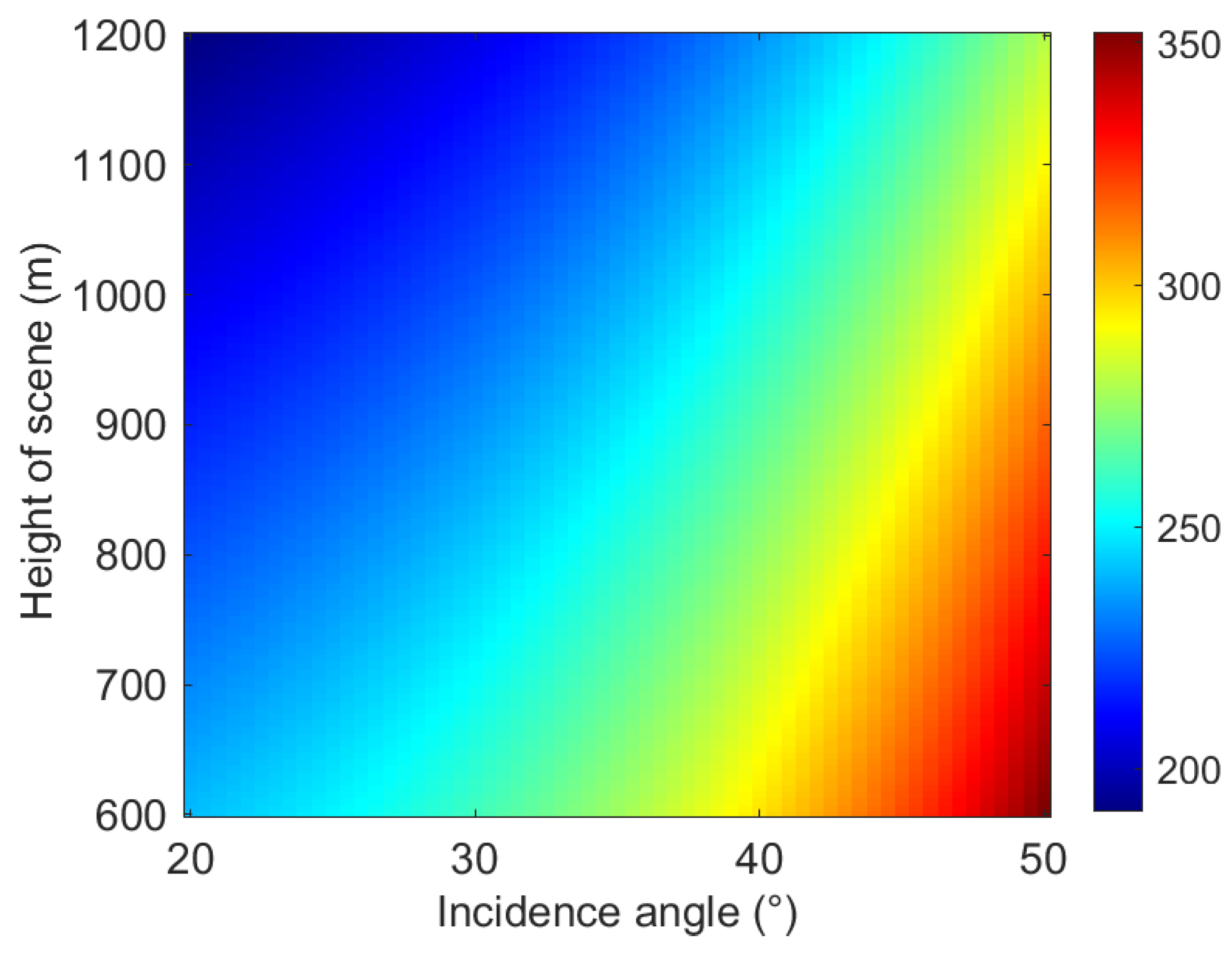
Referring to the flight experiments, let the incidence angle $\theta$ vary from ${20}^{\circ }$ to ${50}^{\circ }$ and the scene height vary from 600 m to 1200 m. The ambiguous elevation map of our system is shown in Figure 2. It can be seen that the ambiguous elevation of the TomoSAR system is determined by the incidence angle and the height of the observation scene. For the test parameter setting, the maximum ambiguous elevation is 352 m, which is smaller than the scene span. This reveals that the original point cloud will be corrupted by elevation ambiguity.

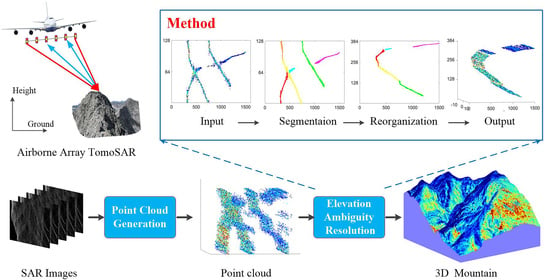
The process of 3D mountain reconstruction using the airborne array TomoSAR is shown in Figure 3. It can be seen that elevation ambiguity resoltion is a necessary step for TomoSAR 3D mountain recontruction. In the following sections, the distribution law of TomoSAR point cloud will be discussed. Furthermore, the proposed elevation ambiguity resolution method and the experimental results will be introduced in detail.

3. Distribution Law of TomoSAR Point Cloud

In this section, the geometric distortion caused by TomoSAR side-view observation is first illustrated. Then, the CS-based layover solution is given. Furthermore, the cause of the elevation ambiguity problem, as well as the problems of intersection and hole in the original point cloud are explained. At last, the distribution law of TomoSAR point cloud is summarized.

3.1. Geometric Distortion

Radar exploits the time required for the electromagnetic wave to go back and forth to the target to measure the range. Under the far-field assumption, the electromagnetic wave can be regarded as a plane wave. For flat ground, the range increases with the ground range. There is only one echo of the scattering center in an azimuth-range unit. However, for uneven surfaces, geometric distortion may occur.

There are three kinds of geometric distortion in SAR images, including foreshortening, layover, and shadowing [28]. The schematic of geometric distortion is shown in sequence in Figure 4, where S indicates the location of radar sensor, $\theta$ indicates the incidence angle, and the red solid line indicates the imaging plane of the observed scene. Foreshortening means that the length of the range displayed on the SAR image is shorter than its real length. As shown in Figure 4a, when the front slope ($ab$: along the projection direction of the SAR beam) is less than the incidence angle $\theta$ or the back slope ($bc$: opposite to the projection direction of the SAR beam) is less than $\pi /2-\theta$, foreshortening occurs. In this case, the front slope shrinks more severely than the back slope. As shown in Figure 4b, layover refers to the phenomenon that the range of the top is smaller than the range of the bottom on the SAR image. This is mainly because the front slope is greater than the incidence angle. In this case, the incident wave first reaches the top and then reaches the bottom. On the imaging plane, $b^{\prime }$ and $a^{\prime }$ are the starting and ending range of a layover region, respectively. As a result, multiple targets with different elevations fall in one azimuth-range unit. Moreover, the electromagnetic wave propagates in a straight line. As shown in Figure 4c, when $\theta +\alpha \ge \pi /2$, there is a section of terrain ($bcd$) behind the front slope that the radar beam cannot reach, and there will be no radar echo. In this case, there is a dark area in the corresponding position of the image ($b^{\prime }{d}^{\prime }$), i.e., shadowing occurs.

3.2. Compressive Sensing-Based Layover Solution

TomoSAR can extend the 2D SAR image to the third elevation dimension through multi-angle observation. The observation geometry on the ground-height plane of the airborne array TomoSAR is shown in Figure 5, where the terrain marked as dark red can be illuminated, and the terrain marked as black indicates the shadowing area. Moreover, the three targets $P_2$, $P_3$ and $P_4$ are layover in an azimuth-range unit. To rebuild them, the pixel value of the complex image can be expressed in the form of superposition of multiple frequency component signals [29]:

$$u(x,r,s_k^{\prime })={\int }_{-S_1/2}^{+S_1/2}\gamma (x,r,s)e^{-j\frac{4\pi }{\lambda }R(s_k^{\prime },s)}ds$$

(2)

where $-S_T/2\le s_k^{\prime }\le S_T/2$, $S_T$ is the overall baseline length, $S_1$ is the elevation span of the illuminated layover terrain, $\gamma$ is the 3D scattering coefficient.

Under far-field approximation, the range function can be expanded in the Taylor series as follows:

$$R(s_k^{\prime },s)\approx R_0+k{b}_{//}+{(s_k^{\prime }-s)}^2/\left(2R_0\right)$$

(3)

Discarding $R_0$, (2) can be written as:

$$\tilde{u}\left(s_k^{\prime }\right)\approx {\int }_{-S_1/2}^{+S_1/2}\tilde{\gamma }\left(s\right)e^{-j\frac{4\pi }{\lambda }{s}_k^{\prime }s}ds,-S_T/2\le s_k^{\prime }\le S_T/2$$

(4)

where

$$\begin{array}{cc}\tilde{u}\left(s_k^{\prime }\right)\approx u\left(s_k^{\prime }\right)e^{-j\frac{4\pi }{\lambda }k{b}_{//}}{e}^{-j\frac{2\pi }{\lambda R_0}{s}_k^{\prime 2}}\hfill & \\ \tilde{\gamma }\left(s\right)=\gamma \left(s\right)e^{-j\frac{2\pi }{\lambda R_0}{s}^2}\hfill \end{array}$$

(5)

Note that the elevation s and the antenna $s_k^{\prime }$ constitute a Fourier pair. Thus, $\tilde{\gamma }\left(s\right)$ can be estimated through an inverse Fourier transform operator. However, this operation requires the baseline to be evenly distributed. Moreover, the Nyquist sampling theorem illustrates that the elevation resolution of the limited number of baselines is limited. Compressed sensing theory can break through the above limitations. If $\tilde{\gamma }\left(s\right)$ can be expressed by the sparsity basis $\left\{{\psi }_i\left(s\right)\right\}$, (4) can be written as:

$$\tilde{\mathit{u}}=\Phi \Psi \mathit{\alpha }$$

(6)

where $\mathit{\alpha }={[{\alpha }_{-(N-1/2)}\dots {\alpha }_{(N-1)/2}]}^T$ is the column vector with K-nonzero elements, $\Psi =\left[{\psi }_{-(N-1/2)}\right|\dots \left|{\psi }_{(N-1)/2}\right]$ is the sparsity sparsis matrix, that is usually expressed as identity matrix, and N is the discrete number in a $2\pi$ period.

The generic element of the measurement matrix $\Phi$ is defined as:

$${\Phi }_{kn}=\frac{1}{\sqrt{N}}{e}^{-j\frac{2\pi h}{N}k}$$

(7)

where $k=1,\dots ,M,h=1,\dots ,N$.

If the signal is K sparse in elevation, and the measurement matrix $\Phi$ satisfies the RIP, the optimal solution of K non-zero coefficients can be obtained through M measured values.The layover solution can be acquired by solving an ${\ell }_1$-norm minimization problem:

$$\widehat{\mathit{\alpha }}=argmin{\parallel \alpha \parallel }_{1}subjectto\tilde{\mathit{u}}=\Phi \Psi \mathit{\alpha }$$

(8)

3.3. Cause of Elevation Ambiguity

Generally, the flat-earth phase between channels is compensated before the generation of point cloud. Therefore, the elevation of ground is zero, and the elevation of the targets on the ground is the relative elevation to the ground. Thus, the original point cloud of regular buildings is distributed in a Z shape [24]. However, for the mountain area with undulating terrain, the elevation of the original point cloud no longer increases monotonically with the ground.

In fact, the phase difference between two adjacent channels $({\phi }_0=-j\frac{4\pi }{\lambda }{b}_{//})$ is a variable related to the incidence angle. That is because the horizontal baseline between the adjacent channels can be expressed as:

$$b_{//}=\frac{2Nbsin(\theta -\beta )}{\lambda }$$

(9)

where $\beta$ is the horizontal angle of the baseline b.

If the flat-earth phase compensation is not done, then the elevation of targets can be expressed as

$$h=\frac{2N{b}_{//}}{\lambda }sin(\theta -\beta )$$

(10)

Discarding the constant variable $\beta$, the above formula can be written as:

$$h=\frac{2N{b}_{//}}{\lambda }sin\theta$$

(11)

Thus, there is a positive correlation relationship between the elevation and the incidence angle. This relationship is called positive correlation constraint in the following. Although the terrain is undulating, the elevation of the point cloud will monotonically increase with the ground.

For the mountain scene shown in Figure 5, the elevation span is $S_T=\frac{2N{b}_{//}}{\lambda }(sin{\theta }_8-sin{\theta }_1)$, where ${\theta }_1$ is the incidence angle of $P_1$, and ${\theta }_8$ is the incidence angle of $P_8$. Based on the spectral estimation, the estimated elevation of the target with the true elevation value $h_t(h_t>N)$ is:

$$h=h_t-dN,h=1,\dots ,N,d\in Z$$

(12)

where d is the number of elevation ambiguity. When the scene span is greater than the ambiguous elevation of the system, d is not equal to zero. As a result, the points outside the elevation period will be aliased in the elevation direction.

The schematic diagram of the elevation ambiguity of layover targets is illustrated in Figure 6. Assuming that $P_3$ is located at the origin of the coordinates, i.e., the elevation value of $P_3$ is zero. Because of elevation ambiguity, only the point $P_3$ in the main period can be correctly sampled, and the points $P_2$ and $P_4$ outside the main period are aliased. The elevation value of $P_2$ is shifted upward for one period, corresponding to $P_2^{\prime }$. Furthermore, the elevation value of $P_4$ is shifted downward for one period, corresponding to $P_4^{\prime }$. Besides, the elevation difference between $P_3$ and $P_4$ is an integer multiple of the ambiguous elevation. In the original point cloud, $P_3$ and $P_4^{\prime }$ will intersect at one point.

3.4. Distribution Law of TomoSAR Point Cloud

Considering the positive correlation constraint and the illumination geometric constraint [30], the real point cloud distribution law is summarized as follows:

(1)

The real point cloud satisfies the boundary constraint in the elevation direction. There is a monotonic increasing relationship between the elevation and ground. Therefore, the elevation values of the points without elevation ambiguity are all within the upper and lower elevation boundaries. As shown in Figure 5, the incidence angle of points $P_1$ to $P_5$ increases with the ground. According to (11), the elevation values of points $P_1$ to $P_5$ increase with the ground. Using the reduction to absurdity, if the elevation value does not increase with the ground distance, $P_6$ will be illuminated. Since $P_6$ is located in the shadow area, it cannot be illuminated;

(2)

The real point cloud satisfies the elevation continuity constraint. If there is no shadowing, the elevation continuously increases. Otherwise, holes will be included in the point cloud. However, the near end and the far end of the hole area have equal elevation values. As shown in Figure 5, there is a shadowing between $P_5$ and $P_7$. The incidence angles of points $P_5$ and $P_7$ are the same. In the same way, the elevation values of points $P_5$ and $P_7$ are the same. Thus, the elevation continuity of the real point cloud is always satisfied.

The distribution law of the original point cloud with elevation ambiguity is summarized as follows:

(1)

The elevation difference between the real target and the ambiguity target is an integer multiple of the discrete numbers in an elevation period;

(2)

The layover points whose elevation difference is an integer multiple of the discrete number will intersect;

(3)

For the points in the same period, the elevation is increasing, and the elevation ambiguity number is equal;

(4)

The elevation values of the points at the near end and the far end of the hole area are continuous.

In summary, the TomoSAR mountain point cloud is affected by geometric distortion and elevation ambiguity. The former is an inherent problem of side-viewing TomoSAR. The latter appears when the elevation span of the illuminated scene is greater than the ambiguous elevation of the TomoSAR system. The intersection is caused by elevation ambiguity and terrain layover. Based on the positive correlation constraint and the illumination geometric constraint, the real point cloud satisfies the boundary constraint and elevation continuity constraint. It is worth emphasizing that the two constrains are not impacted by holes caused by shadowing.

4. The Segmentation and Reorganization-Based Method

In this section, the proposed elevation ambiguity resolution method based on segmentation and reorganization of TomoSAR point cloud is introduced in detail. The workflow of the proposed method is shown in Figure 7.

4.1. Segmentation

The purpose of segmentation is to cluster the points with the same elevation ambiguity number into one category. Segmentation allows the dimensionality reduction from point to category. This idea cannot only improve the efficiency, but also increase the accuracy of the results from a statistical perspective. Considering the outliers and the intersection, the segmentation method combining DBSCAN and GMM is proposed.

First, DBSCAN is performed for all points. Considering the high anisotropy of the positioning error of TomoSAR points, vortex instead of sphere is adopted to determine the neighborhood. By setting the size of vortex and the minimum number of points to be involved in the vortex, the points are divided into three types: core points, boundary points, and outliers. All core points or boundary points connected in density will be clustered into one category. Figure 8a describes DBSCAN, where the voxels are simplified into rectangular windows. The length in the azimuth direction, the width in the range direction, and the height in the elevation direction are marked as $\mathrm{awin}$, $\mathrm{rwin}$ and $\mathrm{hwin}$, respectively. The minimum number of points is marked as $\mathrm{Minpts}$. Points ${\mathrm{p}}_{\mathrm{a}}$ and ${\mathrm{p}}_{\mathrm{b}}$ are density connected to each other since there is a chain of points between them.

Then, denoising is performed. After DBSCAN, the category information is added to the points, and the outliers are marked by a prior label. Meanwhile, some points that are not considered as outliers but do not conform to the terrain trend can be grouped into categories different from that of targets. By setting the removal label, the unwanted points can be removed.

DBSCAN is damaged by intersection. As a result, the points from different elevation periods but connected in density will be clustered into one category, i.e., abnormal category. It is impossible to obtain the correct result by performing the same elevation shift on the abnormal category. When the abnormal category appears in the segmentation result, the second GMM-based clustering will be executed. As shown in Figure 8b, the distribution model of the points is assumed to be a linear combination of K-single Gaussian models. The clustering algorithm based on the distribution model can describe complex spatial shapes. In fact, the abnormal points belong to different elevation periods corresponding to different terrain. That is to say, the abnormal categories can be divided into categories satisfying different distributions by GMM. In this paper, the 2D position information of the range and the elevation is used as the input feature vector. The Bayesian Information Criterion (BIC) is used to estimate the optimal number of category [31]. Meanwhile, the Expectation Maximum (EM) algorithm is used to determine the coefficients of the GMM [32].

Finally, the two-step clustering results will be merged to acquire the segmentation result.

4.2. Reorganization

The purpose of reorganization is to automatically move the points to the correct elevation position. First, the segmentation result is extended in the elevation direction. To elaborate, the segmentation result will be copied on $N_{am}$ adjacent elevation periods. $N_{a}m$ is the elevation span of the processing slice, which is equal to the rounding up of the ratio of the elevation span to the elevation ambiguity of the TomoSAR system. Elevation extension ensures that all points are moved to the correct elevation period. However, the downside is that all points will also be moved to the error periods, and the categories are independent.

Then, a combination is performed for all the categories obtained from elevation extension. The combination ensures that each basic event contains all categories, but the same category does not repeat. Suppose that the number of categories after segmentation is $N_c$. The total number of basic events is $N_{am}^{N_c}$. Among them, one and only one basic event represents the real point cloud distribution, which is called the optimal basic event in the following.

Finally, the basic events that do not satisfy the boundary constraint and the elevation continuity constraint are eliminated. Performing boundary constraint, the basic events whose all points are within the elevation boundary are retained. These boundary values are obtained by specifying the start category and the end category. Because some interference events also comply with boundary constraint, elevation continuity constraint is further applied. According to the spatial continuity, the real point cloud without terrain occlusion is continuous on the ground-elevation plane. Although the continuity may be corrupted by shadowing, the near-end and the far-end of holes are continuous in the elevation direction. Therefore, the elevation continuity is effective even for the complex terrain with shadowing. Considering the impact of missed detection, the maximum elevation difference of the optimal basic event is the smallest of all basic events.

Here, the advantages of geometric constraints are explained. As mentioned above, the total number of basic events depends on the elevation ambiguity number and the number of segmentation categories. The former is an inherent parameter jointly determined by the system ambiguous elevation and the observation scene elevation span. The latter cannot exceed the lower limit, that is, the optimal number of segmentation categories is equal to the elevation ambiguity number. So, the total number of basic events is greater than one. If geometric constraints are not used, the processor needs to interpret and judge one by one from all the reorganization results. Instead, the geometric constraints given in this paper helps to automatic eliminate the interfering basic events, which significantly improves the extraction efficiency of the real point cloud.

5. Experimental Results and Analysis

In this section, the results from both simulated and real data are presented to validate the effectiveness of the proposed method. Furthermore, the 3D reconstruction results of Huangniba Mountain area are presented.

5.1. Simulation Experiments

5.1.1. Data Set

For quantitative evaluation, the simulated TomoSAR mountain point cloud is generated. The global AW3D30 DSM is used to simulate the real 3D coordinates of the tested scene. The AW3D30 DSM data was developed from 3 million scene archives acquired by the PRISM panchromatic stereo mapping sensor on the Advanced Land Observing Satellite “DAICHI” (ALOS) operated from 2006 to 2011 [33,34]. Moreover, it can be downloaded from Japan Aerospace Exploration Agency Earth Observation Research Center 2015 (http://www.eorc.jaxa.jp/ALOS/en/aw3d30/data/index.htm, accessed on 10 December 2021). POV-ray [35] is used to simulate the 3D coordinates and the scattering intensity of the receiving targets. The simulation parameters refer to the parameters of the real airborne array TomoSAR system listed in Table 1. Focusing on the challenge introduced by intersection, a typical subscene is selected. The subscene and its true point cloud on range-elevation plane are shown in Figure 9a,b. The height of the subscene ranges from about 550 m to 950 m. Both elevation ambiguity and intersection are included in the point cloud. Besides, the color maps in Figure 9a,b represent scattering intensity. The scattering intensity of the front slope is higher than that of the back slop.

The simulated original point cloud after weak scattering filtering is shown in Figure 9c. SAR imaging, image registration, and the CS-based layover solution are performed to generate the original point cloud [29]. The number of discrete points in an elevation period is 128. As can be seen, the original point cloud is corrupted by noise and outliers in the elevation direction. In addition, shadowing leads to holes in the original point cloud. For subsequent quantitative evaluation, it is necessary to determine the reference true value. Considering that the position error of TomoSAR points is highly anisotropic, the points that fall in the voxel of the true value are regarded as the reference true value. Similar to the previous definition, the voxel parameters used for estimating the reference true value are set as: $\mathrm{awin}=1$, $\mathrm{rwin}=1$, and $\mathrm{hwin}=2$. Figure 9d presents the reference true value. Specially, the points coded with −1 are regarded as outliers and the other points are regarded as target points. Further, the code of the target points is equal to the elevation ambiguity number.

5.1.2. Segmentation Results

The results of DBSCAN, TSAC, GMM, and the proposed segmentation method are shown in Figure 10, where the different categories are color-coded. DBSCAN is applied for all points with parameter settings: $\mathrm{awin}=1$, $\mathrm{rwin}=1$, $\mathrm{hwin}=2$, and $\mathrm{Minpts}=8$. The parameters are empirically chosen according to the data set. The influence of parameters on the clustering effect has been discussed in [14].

Figure 10a intuitively reveals the difficulties caused by intersection. DBSCAN helps in removing outliers and produce categories without density connected. However, DBSCAN may cluster the points from different elevation periods into one category. The green-coded density connected abnormal category needs to be further segmentated. TSAC is a method that allows to divide the density connected categories of buildings. Notwithstanding, the method is not effective for mountain point cloud (see Figure 10b). The intermediate results of TSAC are shown in Figure 11. Figure 11a is the Gaussion image, which implies that the points density in the Gaussian image domain is uneven. Then, MS are applied for the lower density points, the corresponding Gaussian image and the range-elevation map are represented by Figure 11b,c in turn. It can be seen that the removal of low-density points will lead to false alarm. In addition, the high variability of mountain terrain makes the normal vector has small inter-class differences. In order to separate the points with different elevation periods, TSAC is bound to be over-segmented. From Figure 10c GMM can guarantee correct segmentation, but it saves outliers. Luckily, the proposed segmentation method not only can achieve correct segmentation, but also can suppress outliers.

Purity and the number of categories are used for quantitative analysis of the segmentation results. The closer the purity is to 1, the better the segmentation performance. Besides, under the premise of correct segmentation, the smaller the non-negative difference between the number of segmentation category and the optimal number of category, the better the segmentation performance. That is to say the number of segmentation category should not be less than the elevation span.

The segmentation performance is listed in

Table 2. Segmentation parameters.

	DBSCAN	TSAC	GMM	Proposed
Purity	0.76	0. 92	0.91	0.93
$N_c$	3	10	8	6

. DBSCAN is not robust to intersection. Consequently, the purity of DBSCAN drops to 0.76. The purity for TSAC, GMM, and the proposed method is 0.90, 0.91, and 0.93 in that order. The number of segmentation category for TSAC, GMM, and the proposed method is 10, 8, and 6 in that order. Although the purity of TSAC and GMM is over 0.90, the number of segmentation category is greater than that of the proposed method. Obviously, the proposed method has the highest purity, and the number of segmentation category is closest to the optimal number.

5.1.3. Reorganization Results

Motivated by segmentation, all possible results of elevation ambiguity resolution can be obtained by reorganization. For the simulated point cloud, the elevation span is 3, and the number of category equals to 6. Without any constraints, the number of basic events is 729, equal to the sixth power of three. This also means that in the worst case, 729 selections are needed to obtain the real point cloud. Performing boundary constraint and continuity constraint, the number of basic events is reduced to 243 and 1. In summary, constraints contribute to quickly obtain the optimal basic event.

The results of the elevation ambiguity resolution acquired by region growing [36] and our method are shown in Figure 12. Regardless of outliers, the point cloud acquired by elevation extension is used as the input of region growing. In this paper, the seeds are selected by human–computer interaction. Using the same neighborhood criteria as DBSCAN, and the points in the voxel are all targets by default. Because of intersection, the density-based region growing fails to solve the problem of elevation ambiguity. Intuitively, when encountering intersection, the growing direction may be wrong. With the help of segmentation, this problem is solved by our method.

A point-by-point comparison method is adopted to evaluate the performance of the methods for solving the problem of elevation ambiguity. Similar to the evaluation metrics [37], the performance is then assessed by the following:

$$\begin{array}{c}Completeness(\%):comp=100\times \frac{T_{pp}}{pp+np}\hfill \\ Correctness(\%):corr=100\times \frac{T_{pp}}{pp+pn}\hfill \\ Quality(\%):Q=100\times \frac{comp\times corr}{comp+corr-comp\times corr}=100\times \frac{T_{pp}}{(2pp-Tpp)+pp+pn}\hfill \end{array}$$

(13)

where $pp$ represents the number of points that are both the targets and are correctly extracted; $pn$ represents the number of points that are noise but are extracted; $np$ represents the number of points that are targets but are not extracted; $nn$ represents the number of points that are noise and are not extracted; $Tpp$ represents the number of points belonging to $pp$ and are truly resolved elevation ambiguity.

The performance of elevation ambiguity resolution is listed in

Table 3. Performance of elevation ambiguity eesolution.

	np	pn	pp	Tpp	comp (%)	cor (%)	Q (%)
Reg.	78	292	6548	5310	90.14	77.63	65.11
Pro.	78	292	6548	6461	97.51	94.46	92.23

. Since the input point clouds of the two methods are same, $np$, $pn$ and $pp$ are same. They are mainly determined by DBSCAN, and does not affect the performance comparison of the two methods. Due to the influence of intersection, the $Tpp$ in the result of region growing is significantly smaller than the $Tpp$ in the result of our method. Therefore, the performance indicators of region growing are all significantly inferior to those of our method. For the detected target points, the completeness of region growing and the proposed method is 90.14% and 97.51%, respectively. That is to say, the performance of the elevation ambiguity resolution is significantly improved by the proposed method.

5.2. Real Experiments

5.2.1. Data Set

The real data was obtained by our airborne array TomoSAR experiment in 2019. The 2D SAR image of the tested scene is shown in Figure 13. The size of the scene is 7500 × 6800 (azimuth × range). The pixel sizes in the azimuth direction and the range direction are 0.1133 and 0.1362 m, respectively. Foreshortening, layover (the pixels with brighter scattering intensity), and shadowing (the pixels with dark scattering intensity) are all presented in the scene.

To illustrate problem, the subscene in the rectangular box is selected for a detailed introduction and analysis. The size of the scene is 4000 × 6800 (azimuth × range). Considering the efficiency of data processing and the distribution of layover, partition processing is necessary. The coordinate of the upper left corner of $Rec1$ is $(3500,1)$. The sizes of $Recs1$-5 are 1500 × 2000, 1000 × 2000, 900 × 2000, 1000 × 2000, and 1300 × 2000, respectively. The coordinate of the upper left corner of $Rec6$ is $(5500,2001)$. The sizes of $Recs6$-9 are 1500 × 2000, 1000 × 2000, 1000 × 2000, and 1700 × 2000, respectively. In $Rec1$, $Rec2$, $Rec4$, and $Recs6$-8, the layover is more prominent than shadowing. In $Rec3$, $Rec65$, and $Rec9$, shadowing is more prominent than layover.

The area with elevation ambiguity accounts for 64.22% of the subscene. According to the elevation span and the number of abnormal category, the original point cloud with elevation ambiguity can be divided into five categories (see Figure 14). Taking Figure 14a as an example, the points of slice 1 are from two elevation periods, and the points belong to different elevation periods don’t intersect. Thus, for slice 1, the elevation span is 2, and the number of abnormal category is 0. Similarly, for slices 2–5, the elevation span is 3, 2, 3, and 3, respectively, and the number of abnormal category is 0, 1, 1, and 2, respectively. Their SAR images are indicated with the straight lines in Figure 13. The slices 1–2 represent the case without intersection. The slices 3–5 represent the case with intersection. We carry out the processing of the five slices.

5.2.2. Segmentation Results

Figure 15 shows the segmentation results of DBSCAN, TSAC, GMM, and the proposed segmentation method. The results of the methods are arranged from left to right, and the slices 1–5 are given from top to bottom. Moreover, the different categories are color-coded. The parameters of DBSCAN for slices 1–3 are set as: $\mathrm{awin}=5$, $\mathrm{rwin}=10$, $\mathrm{hwin}=2$, and $\mathrm{Minpts}=8$, and those for slices 4–5 are set as: $\mathrm{awin}=5$, $\mathrm{rwin}=16$, $\mathrm{hwin}=2$, and $\mathrm{Minpts}=8$.

For the case without intersection, there is no need to perform the secondary clustering. So, the methods based on DBSCAN have the same segmentation results. Moreover, they are superior to GMM in terms of noise suppression and segmentation performance.

For the case with intersection, DBSCAN fails to segment the points that are from different elevation periods but connected in density. TSAC also fails even performing clustering in Gaussian image domain. Compared with the simulated data, the read data endures more serious noise interference. TSAC almost only realizes the segmentation of edge points and internal points, rather than the segmentation of abnormal category. Therefore, the third step of clustering is not performed. GMM has outstanding advantages in the segmenting of abnormal category. However, the outliers are saved. Besides, the global clustering makes the number of segmentation category of GMM more than the method in this paper. This goes against the original intention of segmentation. Regardless of whether the cases have intersection, only the method in this paper can achieve correct segmentation.

5.2.3. Reorganization Results

For our method, reorganization is an ingenious method to get the real point cloud from the segmentation results.

Table 4. The number of basic events during the reorganization process.

	Combination	Boundary Constraint	Continuity Constraint
slice 1	8	2	1
slice 2	27	1	1
slice 3	64	8	1
slice 4	6561	6561	1
slice 5	729	729	1

lists the changes in the number of basic events during the reorganization process. Without any constraints, the number of basic events from slice 1 to slice 5 is 8, 27, 64, 6561, and 729, respectively. For slice 4, in the worst case, 6561 selections are required to extract the real point cloud. Based on two-step geometric constraint, the optimal basic event of all slices can be extracted at one time.

The results of the elevation ambiguity resolution acquired by region growing and our method are shown in Figure 16. It can be seen that region growing is only suitable for the slices without intersection. The method in this paper is not only suitable for non-intersecting situations, but also robust to intersecting situations.

Figure 17 shows the 3D point clouds before and after the elevation ambiguity resolution. The original point cloud, the real point cloud in radar coordinate system, and the real point cloud in geodetic coordinate system are presented from left to right, and the slices 1–5 are given from top to bottom. Obviously, the original point cloud is severely distorted in the elevation dorection. After elevation ambiguity resolution, the real structure of mountains will be reconstructed. It can be concluded that elevation ambiguity resolution of TomoSAR point cloud is a necessary step in 3D reconstruction.

Furthermore, external data is used to prove the correctness of the elevation ambiguity resolution. Figure 18 presents the real point cloud, the Elevation Position Result (EPR), the DSM data and the 1:10,000 DEM data. The original grid sizes of the two external data are inconsistent and are much larger than the horizontal resolution of the reconstruction results. Thus, the DSM and DEM data presented in this paper have been interpolated by Global Mapper, and the grid size is 1 × 1 m. The terrain trends presented by the real point cloud and the two external data are almost same, which indicates that the proposed method for solving elevation ambiguity is effective. Moreover, quantitatively evaluation of the EPR results is performed. The height precision (the average height distance of an estimated point to the ground truth surface) of slices 1–5 is 4.02 m, 3.17 m, 14.06 m, 5.68 m, and 4.51 m, respectively. Although the height precision of slice 3 is somewhat abnormal, it may be mainly affected by the original point cloud and the true value (see the special patch in ground range geometry indicated by a red rectangular box in Figure 18) rather than our method. Therefore, it can be concluded that the results of the elevation ambiguity resolution are correct.

As mentioned above, the values of DEM and DSM may deviate greatly. Here, the issue of which kind of external data can be selected as the true value is described in detail. Since both DSM and TomoSAR processing results characterize the height of ground objects, DSM are mainly used as the true value. In theory, the height value of DSM is not less than that of DEM. However, in the actual processing results, the height value of DSM may less than that of DEM. Considering that the grid size of the DEM data is smaller than that of DSM, for the terrain where DEM is higher than DSM, the DEM data is taken as the true value. It is worth emphasizing that no matter which data is chosen as the reference true value, it does not affect the conclusion that the proposed method is effective for the elevation ambiguity resolution.

5.3. 3D Mountain Reconstruction Results

In Figure 19, the optical image of the reconstruction area is marked by a red rectangle. The latitude and longitude are $({103}^{\circ }{30}^{\prime }{42}^{″}\mathrm{E}\sim {103}^{\circ }{31}^{\prime }{11}^{″}\mathrm{E},{29}^{\circ }{24}^{\prime }$${41}^{″}\mathrm{N}\sim {29}^{\circ }{25}^{\prime }{27}^{″}\mathrm{N})$. The size of the scene is 800 m × 1400 m (azimuth × ground). The reconstruction area is located in the Huangniba mountain area, Leshan City, Sichuan Province, China. The Huangniba mountain area is located in the north-western region of the Desheng Square in Shawan District, Leshan City. As shown in Figure 19, the distance between the location marked Peak 1 and the Desheng Square is about 4.2 km in the east–west direction and 1.6 km in the north–south direction.

Figure 20 shows the 3D reconstruction image obtained by DSM and the process of this paper. The color map represents the height. Figure 20a,b are the stereograph and the top view of the DSM, respectively. Figure 20c,d are the stereograph and the top view of the image of this paper, respectively. Median filter, grid interpolation (1 m × 1 m) and smoothing are performed to the results of elevation ambiguity resolution. The 3D reconstruction image obtained in this paper is basically consistent with the optical image and the image from AW3D30 DSM: two main peaks are, respectively, located on the north and east sides of the test scene, and there are obvious depressions between the two peaks; There is a depression in the middle of Peak 1; both the height variation range of our image and AW3D30 DSM are 600 to 1200 m.

Affected by shadowing, there are many holes in the original point cloud. Becasue of interpolation processing, the height error in the hole area is very large. Not only will the elevation precision of the local area be reduced, but it is also very unfavorable for the subsequent quantitative evaluation. Scattering intensity is the fourth-dimension information reflecting the echo intensity of the observed scene. Figure 21 shows the 3D image with scattering information. The horizontal and vertical coordinates indicate latitude and longitude information. To enhance the image contrast, the scattered intensity is truncated and normalized. It can be seen that the scattering information helps to identify hole areas and terrain texture. The scattering intensity of the front slope is greater than that of the back slope. Affected by shadowing, the scattering intensity of the back slope is mostly zero. Besides, our images can well recover the detailed information of the ground object scattering. The 3D image produced by AW3D30 DSM data and Google Earth and the 3D image obtained from array TomoSAR are compared under different viewing angles. The comparison images are shown in Figure 22. The terrain trend presented by the two images are almost the same. Specifically, a smooth surface on the front slope is contained in the red circle in Figure 22e. In our results, this area is in the red circle in Figure 22f. The scattering intensity of this area is indeed weaker than the scattering intensity of the neighboring areas. In summary, the scattering information is another indicator that confirms the credibility of the reconstruction results in this paper.

The quantitative evaluation of the our results is compared to the DSM. The absolute height erroe map is presented in Figure 23. Figure 23a,b are the stereograph and the top view of the 3D reconstruction image with the absolute height error as the color map. 1:10,000 DEM production technology stipulates that the mean height error of high mountain area is 12.06 m, and the maximum height error of high mountain area is 24.12 m. The absolute height error of the former has not been processed, and the absolute height error of the latter has been truncated with 24.12 m as the critical value. In actual data processing, the points with a scattering intensity less than 0.25 are regarded as noise and removed. Therefore, the area where the scattering intensity is less than 0.25 is regarded as shadowing, and it is not considered by the quantitative evaluation. The absolute height error of the shadowing is marked as −1 m. It can be seen from Figure 23a,b that the absolute height error is relatively large at the shadowing junction. Figure 23c illustrates the histogram of the absolute height error. The percentage of absolute height error less than 24.12 and 12.06 m are, respectively, 96.22% and 86.29%, and the mean absolute elevation error is 6.62 m. It is exciting to note that the absolute height error of our 3D mountain reconstruction results is in accordance with the DEM production techniques. Moreover, the horizontal resolution of the reconstruction results in this paper is much higher than the 5 m resolution of DEM data. In summary, the method proposed in this paper is not only helpful for 3D reconstruction of mountainous areas, but also has guiding significance for high-precision mountain mapping.

6. Conclusions

Three-dimensional (3D) mountain reconstruction is crucial to topographic surveying and mapping, bridge erection, disaster prevention and mitigation, etc. However, the problem of elevation ambiguity makes the original point cloud geometrically deformed. In-depth analysis of geometric distortion and the principle of layover solution, the cause of the difficulties in solving the elevation ambiguity problem is explained. Furthermore, the law of TomoSAR point cloud is derived. Motivated by the elevation boundary constraint and the elevation continuity constraint of TomoSAR point cloud, an elevation ambiguity resolution method is proposed in this paper. The method mainly includes two steps including segmentation and reorganization. The performance of the proposed method is illustrated by both simulated data and the real airborne array TomoSAR data. The comparison with the traditional methods demonstrates that even in the case of intersection, the proposed method is effective. Based on the real results, the 3D mountain images are further presented. The results show that these images with the proposed method have similar topographic features with the optical image, AW3D30 DSM and 1:10,000 DEM. With DSM as the true value, the average elevation error of the 3D reconstruction result is 6.62 m.

There are several aspects of the proposed method that can be improved in the future. Firstly, the automatic identification of abnormal category needs to be further studied. Secondly, if the abnormal category conforms to multiple distributions with large differences, more categories are needed to separate them. This will increase the total number of basic events and increase the difficulty of the optimal basic event extraction. Future work will focus on these factors, and strive to obtain more robust method for solving the problem of elevation ambiguity. Moreover, the high-precision 3D mountain reconstruction using airborne array TomoSAR will also be considered.

References

1. Köninger, A.; Bartel, S. 3D-GIS for urban purposes. Geoinformatica 1998, 2, 79–103. [Google Scholar] [CrossRef]
2. Lu, H.; Zhang, H.; Deng, Y.; Wang, J.; Yu, W. Building 3-D reconstruction with a small data stack using SAR tomography. IEEE J. Sel. Top. Appl. Earth Obs. Remote Sens. 2020, 13, 2461–2474. [Google Scholar] [CrossRef]
3. Minh, D.H.T.; Le Toan, T.; Rocca, F.; Tebaldini, S.; Villard, L.; Réjou-Méchain, M.; Phillips, O.L.; Feldpausch, T.R.; Dubois-Fernandez, P.; Scipal, K.; et al. SAR tomography for the retrieval of forest biomass and height: Cross-validation at two tropical forest sites in French Guiana. Remote Sens. Environ. 2016, 175, 138–147. [Google Scholar] [CrossRef] [Green Version]
4. Chen, F.; Lasaponara, R.; Masini, N. An overview of satellite synthetic aperture radar remote sensing in archaeology: From site detection to monitoring. J. Cult. Herit. 2017, 23, 5–11. [Google Scholar] [CrossRef]
5. Bayer, B.; Schmidt, D.; Simoni, A. The influence of external digital elevation models on PS-InSAR and SBAS results: Implications for the analysis of deformation signals caused by slow moving landslides in the northern apennines (Italy). IEEE Trans. Geosci. Remote Sens. 2017, 55, 2618–2631. [Google Scholar] [CrossRef]
6. Knaell, K.; Cardillo, G. Radar tomography for the generation of three-dimensional images. IEE Proc.-Radar Sonar Navig. 1995, 142, 54–60. [Google Scholar] [CrossRef] [Green Version]
7. Fornaro, G.; Serafino, F. Imaging of single and double scatterers in urban areas via SAR tomography. IEEE Trans. Geosci. Remote Sens. 2006, 44, 3497–3505. [Google Scholar] [CrossRef]
8. Werninghaus, R.; Buckreuss, S. The TerraSAR-X mission and system design. IEEE Trans. Geosci. Remote Sens. 2009, 48, 606–614. [Google Scholar] [CrossRef] [Green Version]
9. Covello, F.; Battazza, F.; Coletta, A.; Lopinto, E.; Fiorentino, C.; Pietranera, L.; Valentini, G.; Zoffoli, S. COSMO-SkyMed an existing opportunity for observing the Earth. J. Geodyn. 2010, 49, 171–180. [Google Scholar] [CrossRef] [Green Version]
10. Fischler, M.A.; Bolles, R.C. Random sample consensus: A paradigm for model fitting with applications to image analysis and automated cartography. Commun. ACM 1981, 24, 381–395. [Google Scholar] [CrossRef]
11. D’Hondt, O.; Guillaso, S.; Hellwich, O. Geometric primitive extraction for 3D reconstruction of urban areas from tomographic SAR data. In Proceedings of the Joint Urban Remote Sensing Event 2013, Sao Paulo, Brazil, 21–23 April 2013; pp. 206–209. [Google Scholar]
12. Wang, Y.; Zhu, X.X. Automatic feature-based geometric fusion of multiview TomoSAR point clouds in urban area. IEEE J. Sel. Top. Appl. Earth Obs. Remote Sens. 2014, 8, 953–965. [Google Scholar] [CrossRef] [Green Version]
13. Zhu, X.X.; Shahzad, M. Facade reconstruction using multiview spaceborne TomoSAR point clouds. IEEE Trans. Geosci. Remote Sens. 2013, 52, 3541–3552. [Google Scholar] [CrossRef]
14. Shahzad, M.; Zhu, X.X. Robust reconstruction of building facades for large areas using spaceborne TomoSAR point clouds. IEEE Trans. Geosci. Remote Sens. 2014, 53, 752–769. [Google Scholar] [CrossRef] [Green Version]
15. Ester, M.; Kriegel, H.P.; Sander, J.; Xu, X. A density-based algorithm for discovering clusters in large spatial databases with noise. In Proceedings of the Second International Conference on Knowledge Discovery and Data Mining (KDD-96), Portland, OR, USA, 2–4 August 1996; Volume 96, pp. 226–231. [Google Scholar]
16. Idrissi, S.E.E.; Villard, L.; Borderies, P.; Koleck, T.; Burban, B.; Le Toan, T. Long-Term Trends of P-Band Temporal Decorrelation Over a Tropical Dense Forest-Experimental Results for the BIOMASS Mission. IEEE Trans. Geosci. Remote Sens. 2021, 99, 1–15. [Google Scholar]
17. Zhang, F.; Liang, X.; Wu, Y.; Lv, X. 3D surface reconstruction of layover areas in continuous terrain for multi-baseline SAR interferometry using a curve model. Int. J. Remote Sens. 2015, 36, 2093–2112. [Google Scholar] [CrossRef]
18. Zhang, F. Research on Signal Processing of 3-D Reconstruction in Linear Array Synthetic Aperture Radar Interferometry. Ph.D. Thesis, University of Chinese Academy of Sciences, Beijing, China, 2015. [Google Scholar]
19. Hang, L.; Xingdong, L.; Fubo, Z.; Yirong, W. 3D imaging for array InSAR based on Gaussian mixture model clustering. J. Radars 2017, 6, 630–639. [Google Scholar]
20. Zivkovic, Z. Improved adaptive Gaussian mixture model for background subtraction. In Proceedings of the 17th International Conference on Pattern Recognition, Cambridge, UK, 26 August 2004; Volume 2, pp. 28–31. [Google Scholar]
21. Zhou, S.; Li, Y.; Zhang, F.; Chen, L.; Bu, X. Automatic Regularization of TomoSAR Point Clouds for Buildings Using Neural Networks. Sensors 2019, 19, 3748. [Google Scholar] [CrossRef] [Green Version]
22. Jiao, Z.; Ding, C.; Qiu, X.; Zhou, L.; Chen, L.; Han, D.; Guo, J. Urban 3D imaging using airborne TomoSAR: Contextual information-based approach in the statistical way. ISPRS J. Photogramm. Remote Sens. 2020, 170, 127–141. [Google Scholar] [CrossRef]
23. Zhang, F.; Liang, X.; Cheng, R.; Wan, Y.; Chen, L.; Wu, Y. Building Corner Reflection in MIMO SAR Tomography and Compressive Sensing-Based Corner Reflection Suppression. IEEE Geosci. Remote Sens. Lett. 2019, 17, 446–450. [Google Scholar] [CrossRef]
24. Cheng, R.; Liang, X.; Zhang, F.; Chen, L. Multipath scattering of typical structures in urban areas. IEEE Trans. Geosci. Remote Sens. 2018, 57, 342–351. [Google Scholar] [CrossRef]
25. Li, M.; Xiang, Y.; Chen, X.; Wang, Y.; Lu, Y.; Ding, Z. Altitude ambiguity suppression method based on dual-frequency interfering and multi-frequency averaging for sparse baseline TomoSAR. Electron. Lett. 2019, 55, 1194–1196. [Google Scholar] [CrossRef]
26. Hensley, S.; Chapman, B.; Lavalle, M.; Hawkins, B.; Riel, B.; Michel, T.; Muellerschoen, R.; Lou, Y.; Simard, M. UAVSAR L-band and P-band tomographic experiments in boreal forests. In Proceedings of the IGARSS 2018—2018 IEEE International Geoscience and Remote Sensing Symposium, Valencia, Spain, 22–27 July 2018; pp. 8679–8682. [Google Scholar]
27. Fornaro, G.; Lombardini, F.; Pauciullo, A.; Reale, D.; Viviani, F. Tomographic processing of interferometric SAR data: Developments, applications, and future research perspectives. IEEE Signal Process. Mag. 2014, 31, 41–50. [Google Scholar] [CrossRef]
28. Walterscheid, I.; Espeter, T.; Gierull, C.; Klare, J.; Brenner, A.R.; Ender, J.H. Results and analysis of hybrid bistatic SAR experiments with spaceborne, airborne and stationary sensors. In Proceedings of the 2009 IEEE International Geoscience and Remote Sensing Symposium, Cape Town, South Africa, 12–17 July 2009; Volume 2, pp. II-238–II-241. [Google Scholar]
29. Budillon, A.; Evangelista, A.; Schirinzi, G. Three-dimensional SAR focusing from multipass signals using compressive sampling. IEEE Trans. Geosci. Remote Sens. 2010, 49, 488–499. [Google Scholar] [CrossRef]
30. Ley, A.; D’Hondt, O.; Hellwich, O. Regularization and completion of TomoSAR point clouds in a projected height map domain. IEEE J. Sel. Top. Appl. Earth Obs. Remote Sens. 2018, 11, 2104–2114. [Google Scholar] [CrossRef]
31. Vrieze, S.I. Model selection and psychological theory: A discussion of the differences between the Akaike information criterion (AIC) and the Bayesian information criterion (BIC). Psychol. Methods 2012, 17, 228. [Google Scholar] [CrossRef] [PubMed] [Green Version]
32. Moon, T.K. The expectation-maximization algorithm. IEEE Signal Process. Mag. 1996, 13, 47–60. [Google Scholar] [CrossRef]
33. Takaku, J.; Tadono, T.; Tsutsui, K. Generation of high resolution global DSM from ALOS PRISM. ISPRS Ann. Photogramm. Remote Sens. Spat. Inf. Sci. 2014, 2. [Google Scholar] [CrossRef] [Green Version]
34. Takaku, J.; Tadono, T.; Doutsu, M.; Ohgushi, F.; Kai, H. Updates of ‘AW3D30’ALOS Global Digital Surface Model with Other Open Access Datasets. Int. Arch. Photogramm. Remote Sens. Spat. Inf. Sci. 2020, 43, 183–189. [Google Scholar] [CrossRef]
35. Auer, S.; Hinz, S.; Bamler, R. Ray-tracing simulation techniques for understanding high-resolution SAR images. IEEE Trans. Geosci. Remote Sens. 2009, 48, 1445–1456. [Google Scholar] [CrossRef] [Green Version]
36. Adams, R.; Bischof, L. Seeded region growing. IEEE Trans. Pattern Anal. Mach. Intell. 1994, 16, 641–647. [Google Scholar] [CrossRef] [Green Version]
37. Rutzinger, M.; Rottensteiner, F.; Pfeifer, N. A comparison of evaluation techniques for building extraction from airborne laser scanning. IEEE J. Sel. Top. Appl. Earth Obs. Remote Sens. 2009, 2, 11–20. [Google Scholar] [CrossRef]
Figure 1. The 3D observation geometry of the airborne array TomoSAR.
Remotesensing 13 05118 g001
Figure 2. Ambiguous elevation as a function of the incidence angle and the height of scene.
Remotesensing 13 05118 g002
Figure 3. The process of 3D mountain reconstruction using the airborne array TomoSAR.
Remotesensing 13 05118 g003
Figure 4. Schematic of geometric distortion. (a) Forshortening. (b) Layover. (c) Shadowing.
Remotesensing 13 05118 g004
Figure 5. The observation geometry on the ground-height plane of the airborne array TomoSAR. The terrain marked as dark red can be illuminated, and the terrain marked as black indicates the shadowing area.
Remotesensing 13 05118 g005
Figure 6. The schematic diagram of the elevation ambiguity of layover targets.
Remotesensing 13 05118 g006
Figure 7. The workflow of the proposed elevation ambition resolution method.
Remotesensing 13 05118 g007
Figure 8. Illustration of (a) DBSCAN, and (b) GMM.
Remotesensing 13 05118 g008
Figure 9. Simulated scenes: (a) the subscene in ground range geometry; (b) the truth point cloud; (c) the simulated original point cloud; (d) the reference true value. The color maps in (a,c) represent scattering intensity. The colors in (d) represent outliers (−1) and elevation ambiguity number.
Remotesensing 13 05118 g009
Figure 10. Segmentation results of the simulated data: (a) DBSCAN; (b) TSAC; (c) GMM; (d) the proposed segmentation method. The different categories are color-coded.
Remotesensing 13 05118 g010aRemotesensing 13 05118 g010b
Figure 11. The intermediate results of TSAC for the abnormal category in Figure 10: (a) the Gaussian image; (b,c) the Gaussian image and range-elevation map after performing MS for the lower density points; (d) the range-elevation map after performing the third density-based clustering. The color on the left figure represents the density of points, and the color on the other figures represents different categories.
Remotesensing 13 05118 g011
Figure 12. The results of the elevation ambiguity resolution acquired by (a) region growing and (b) our method. The red dots indicate the seeds.
Remotesensing 13 05118 g012
Figure 13. Two-dimensional (2D) SAR image of the tested scene.
Remotesensing 13 05118 g013
Figure 14. Range-elevation maps of the original point cloud: (a) slice 1; (b) slice 2; (c) slice 3; (d) slice 4; (e) slice 5. The colormap represents the normalized scatetring intensity.
Remotesensing 13 05118 g014
Figure 15. Slices on range-elevation plane of the segmentation results. From top to bottom: slice 1 to slice 5. From left to right: DBSCAN, TSAC, GMM, and the proposed segmentation method. The different categories are color-coded.
Remotesensing 13 05118 g015
Figure 16. Slices on range-elevation plane after elevation ambiguity resolution. From top to bottom: slice 1 to slice 5. From left to right: region growing and the proposed method. The red dot represents the seed.
Remotesensing 13 05118 g016
Figure 17. Comparison of the 3D point clouds before and after the elevation ambiguity resolution. From top to bottom: slice 1 to slice 5. From left to right: the original point cloud, the real point cloud in radar coordinate system, and the real point cloud in geodetic coordinate system.
Remotesensing 13 05118 g017
Figure 18. Slices of the real point cloud, the Elevation Position Result (EPR), the DSM data, and the DEM data. The left are the slices on range-elevation plane, and the right are the slices on ground-height plane.
Remotesensing 13 05118 g018
Figure 19. Optical image of the survey area.
Remotesensing 13 05118 g019
Figure 20. Three-dimensional (3D) images of the Huangniba mountain area: (a,b) are the stereograph and the top view of AW3D30 DSM, respectively; (c,d) are the stereograph and the top view of our result, respectively.
Remotesensing 13 05118 g020
Figure 21. Three-dimensional (3D) image of the reconstruction mountain with scattering information.
Remotesensing 13 05118 g021
Figure 22. Three-dimensional (3D) images under different viewing angles: (a,b) are the images under view([114,22]); (c,d) are the images under view([105,40]); (e,f) are the images under view([−115,58]). For view([az,el]), az and el are the azimuth and elevation angles of the line of sight in the geodetic coordinate system. The left images are produced by AW3D30 DSM data and Google Earth. The right images are obtained from array TomoSAR.
Remotesensing 13 05118 g022
Figure 23. (a,b) The stereograph and the top view of the 3D reconstruction image with the absolute height error as the color map; (c) the histogram of the absolute height error.
Remotesensing 13 05118 g023