Displacement Analysis of Geothermal Field Based on PSInSAR And SOM Clustering Algorithms A Case Study of Brady Field, Nevada—USA


Abstract
:1. Introduction
2. The Study Area and the Data
3. The Proposed Methodology
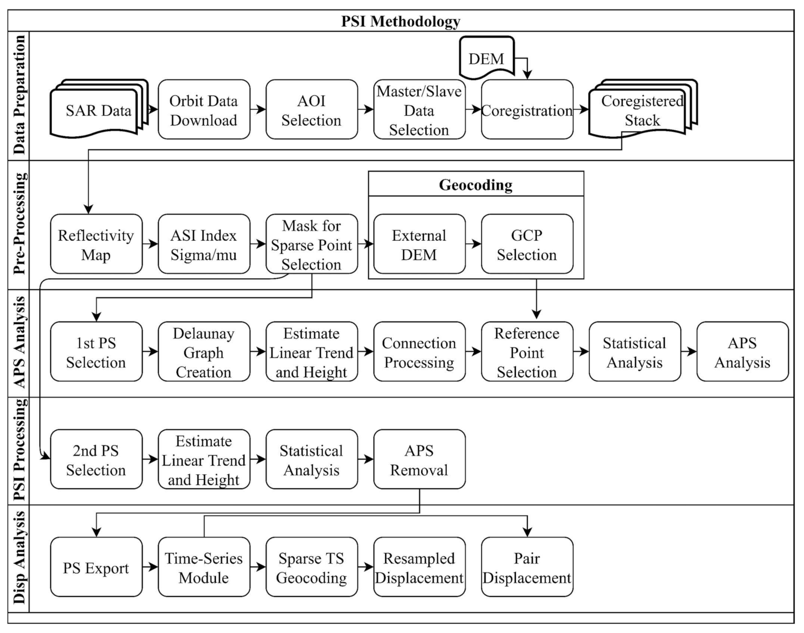
3.1. Step I—Analysis of Displacements Using PSInSAR
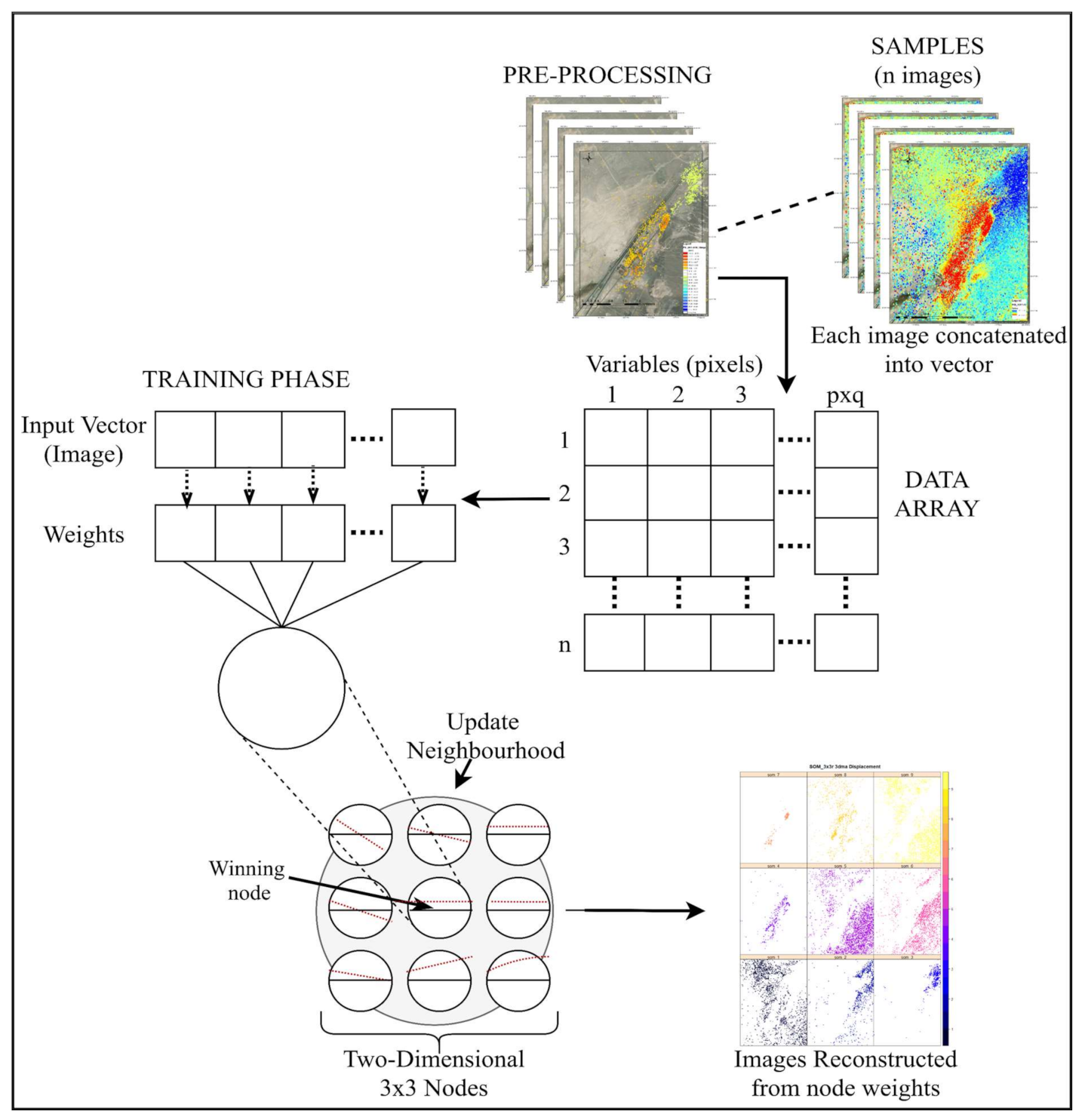
3.2. Step II—Analysis of Spatiotemporal Patterns Using Self-Organizing Map (SOM)
3.3. Step III—Temporal Analysis of Displacements Using the Time-Series from SOM
4. Results and Discussion
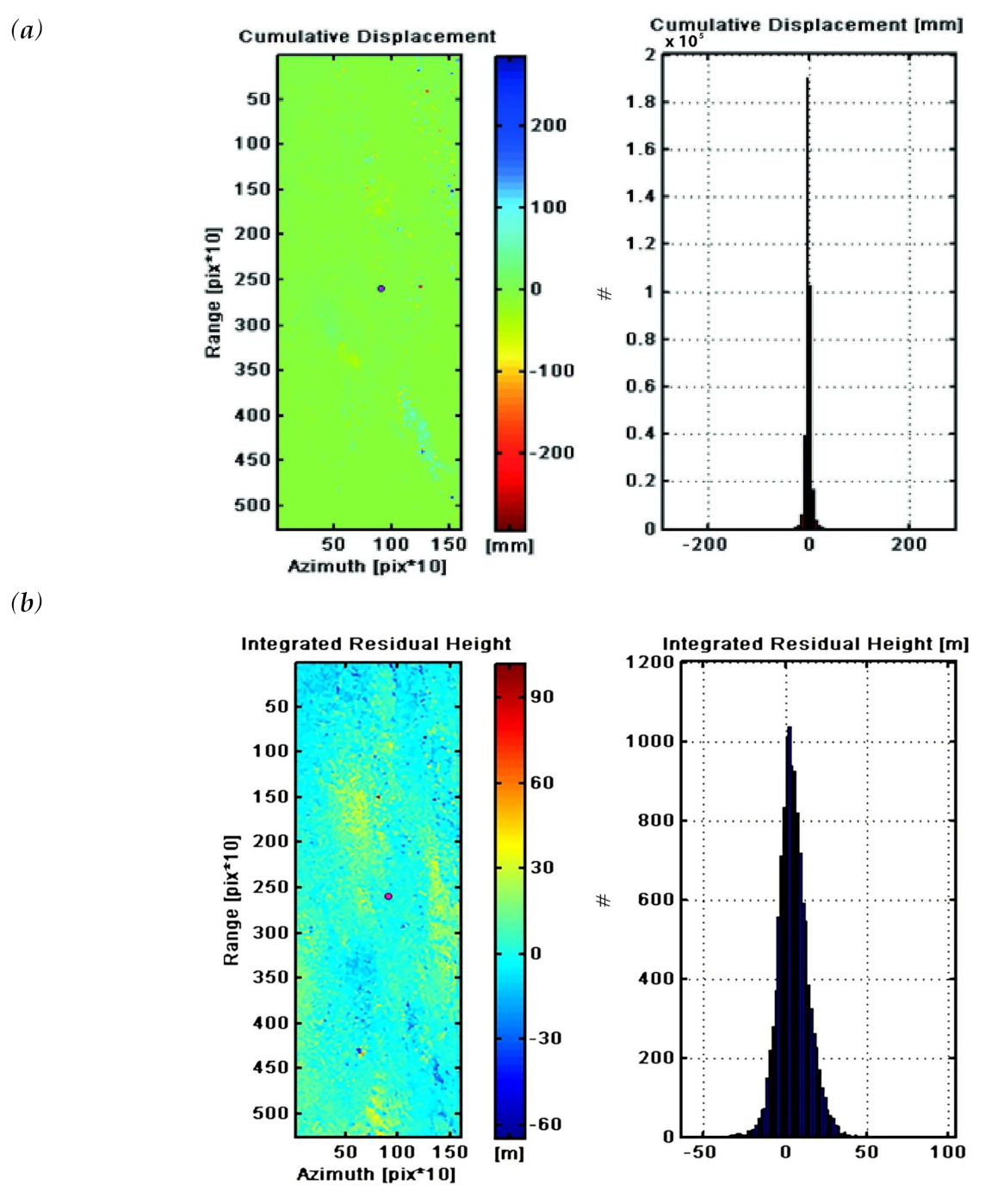
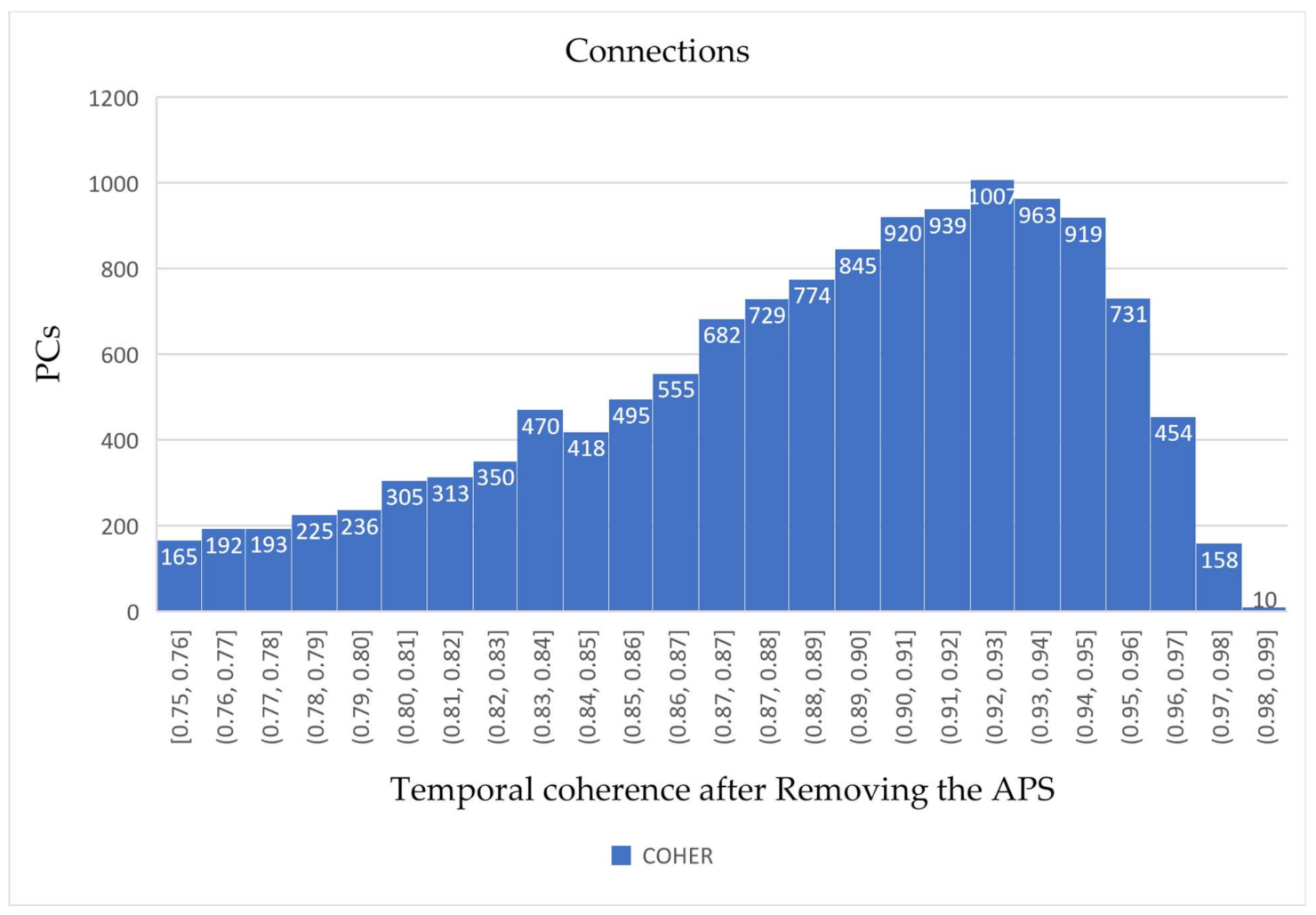
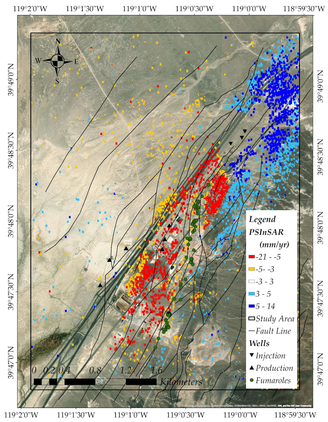
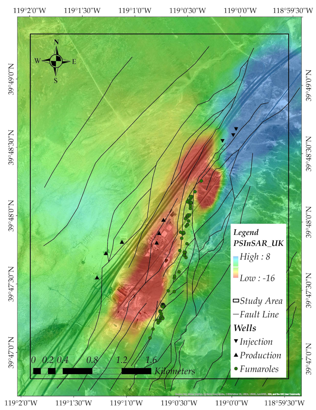
4.1. Step I—The PSInSAR Analysis
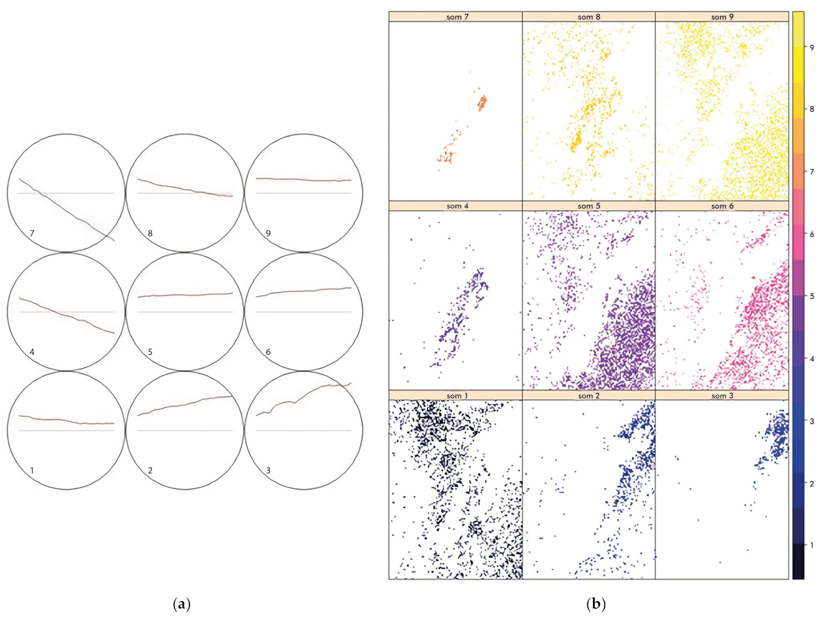
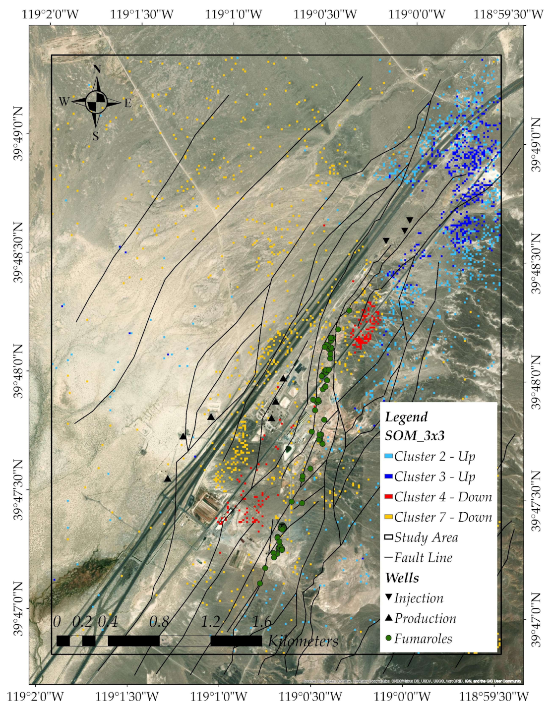
4.2. Step II—The SOM Analysis
4.3. Step III—Temporal Analysis of Displacements
5. Conclusions
Author Contributions
Funding
Data Availability Statement
Acknowledgments
Conflicts of Interest
References
- Békési, E.; Fokker, P.A.; Martins, J.E.; Limberger, J.; Bonté, D.; Van Wees, J.-D. Production-Induced Subsidence at the Los Humeros Geothermal Field Inferred from PS-InSAR. Geofluids 2019, 2019, 1–12. [Google Scholar] [CrossRef]
- Wang, W.; Diessl, J.; Bruno, M.S. Surface deformation study for a geothermal operation field. Adv. Geosci. 2018, 45, 243–249. [Google Scholar] [CrossRef] [Green Version]
- Reinisch, E.C.; Ali, S.T.; Cardiff, M.; Kaven, J.O.; Feigl, K.L. Geodetic Measurements and Numerical Models of Deformation at Coso Geothermal Field, California, USA, 2004–2016. Remote Sens. 2020, 12, 225. [Google Scholar] [CrossRef] [Green Version]
- Manunta, M.; De Luca, C.; Zinno, I.; Casu, F.; Manzo, M.; Bonano, M.; Fusco, A.; Pepe, A.; Onorato, G.; Berardino, P.; et al. The Parallel SBAS Approach for Sentinel-1 Interferometric Wide Swath Deformation Time-Series Generation: Algorithm Description and Products Quality Assessment. IEEE Trans. Geosci. Remote Sens. 2019, 57, 6259–6281. [Google Scholar] [CrossRef]
- Kabeyi, M.J. Geothermal Electricity Generation, Challenges, Opportunities and Recommendations. Int. J. Adv. Sci. Res. Eng. 2019, 5, 53–95. [Google Scholar] [CrossRef]
- Ferretti, A.; Fumagalli, A.; Novali, F.; Prati, C.; Rocca, F.; Rucci, A. A New Algorithm for Processing Interferometric Data-Stacks: SqueeSAR. IEEE Trans. Geosci. Remote Sens. 2011, 49, 3460–3470. [Google Scholar] [CrossRef]
- Lubitz, C.; Motagh, M.; Kaufmann, C. Ground Surface Response to Geothermal Drilling and the Following Counteractions in Staufen im Breisgau (Germany) Investigated by TerraSAR-X Time Series Analysis and Geophysical Modeling. Remote Sens. 2014, 6, 10571–10592. [Google Scholar] [CrossRef] [Green Version]
- Crosetto, M.; Monserrat, O.; Cuevas-González, M.; Devanthéry, N.; Crippa, B. Persistent Scatterer Interferometry: A review. ISPRS J. Photogramm. Remote Sens. 2016, 115, 78–89. [Google Scholar] [CrossRef] [Green Version]
- Cavur, M.; Camalan, M.; Ketizmen, H.; Agitoglu, S. Monitoring of Mine Landslide and Deformation Using Sentinel-1 Sar Data. In Proceedings of the IMCET 2019 26th International Mining Congress and Exhibition of Turkey 2019, Antalya, Turkey, 2019; Benzer, H., Aydogan, N., Karadeniz, M., Altun, O., Dundar, H., Gulsun Kilic, M., Kundak, E., Yilmazkaya, E., Eds.; Baski: Antalya, Turkey, 2019; pp. 509–517. [Google Scholar]
- Bardi, F.; Raspini, F.; Ciampalini, A.; Kristensen, L.; Rouyet, L.; Lauknes, T.R.; Frauenfelder, R.; Casagli, N. Space-Borne and Ground-Based InSAR Data Integration: The Åknes Test Site. Remote Sens. 2016, 8, 237. [Google Scholar] [CrossRef] [Green Version]
- Cigna, F.; Tapete, D.; Hugo, G.-M.V.; Muñiz-Jauregui, J.A.; García-Hernández, O.H.; Jiménez-Haro, A. Wide-Area InSAR Survey of Surface Deformation in Urban Areas and Geothermal Fields in the Eastern Trans-Mexican Volcanic Belt, Mexico. Remote Sens. 2019, 11, 2341. [Google Scholar] [CrossRef] [Green Version]
- Komac, M.; Holley, R.; Mahapatra, P.S.; Van Der Marel, H.; Bavec, M. Coupling of GPS/GNSS and radar interferometric data for a 3D surface displacement monitoring of landslides. Landslides 2014, 12, 241–257. [Google Scholar] [CrossRef]
- Carlà, T.; Raspini, F.; Intrieri, E.; Casagli, N. A simple method to help determine landslide susceptibility from spaceborne InSAR data: The Montescaglioso case study. Environ. Earth Sci. 2016, 75, 75. [Google Scholar] [CrossRef] [Green Version]
- Lu, P.; Catani, F.; Tofani, V.; Casagli, N. Quantitative hazard and risk assessment for slow-moving landslides from Persistent Scatterer Interferometry. Landslides 2013, 11, 685–696. [Google Scholar] [CrossRef]
- Tomás, R.; Li, Z.; Lopez-Sanchez, J.M.; Liu, P.; Singleton, A. Using wavelet tools to analyse seasonal variations from InSAR time-series data: A case study of the Huangtupo landslide. Landslides 2015, 13, 437–450. [Google Scholar] [CrossRef] [Green Version]
- Massonnet, D.; Rabaute, T. Radar interferometry: Limits and potential. IEEE Trans. Geosci. Remote Sens. 1993, 31, 455–464. [Google Scholar] [CrossRef]
- Jónsson, S.; Zebker, H.; Cervelli, P.F.; Segall, P.; Garbeil, H.; Rowland, S.; Mouginis-Mark, P. A shallow-dipping dike fed the 1995 flank eruption at Fernandina Volcano, Galápagos, observed by satellite radar interferometry. Geophys. Res. Lett. 1999, 26, 1077–1080. [Google Scholar] [CrossRef] [Green Version]
- Brandt, J.T.; Sneed, M.; Danskin, W.R. Detection and measurement of land subsidence and uplift using interferometric synthetic aperture radar, San Diego, California, USA, 2016–2018. Proc. Int. Assoc. Hydrol. Sci. 2020, 382, 45–49. [Google Scholar] [CrossRef] [Green Version]
- Carnec, C.; Delacourt, C. Three years of mining subsidence monitored by SAR interferometry, near Gardanne, France. J. Appl. Geophys. 2000, 43, 43–54. [Google Scholar] [CrossRef]
- Crosetto, M.; Monserrat, O.; Barra, A.; Crippa, B. Deformation Measurement Using Sentinel-1a/b Imagery. Int. Arch. Photogramm. Remote Sens. Spat. Inf. Sci. 2017, 42. [Google Scholar] [CrossRef] [Green Version]
- Kim, S.; Lee, C.; Song, K.; Min, K.D.; Won, J. Application of L-band differential SAR interferometry to subsidence rate estimation in reclaimed coastal land. Int. J. Remote Sens. 2005, 26, 1363–1381. [Google Scholar] [CrossRef]
- Alsdorf, D.E.; Melack, J.M.; Dunne, T.; Mertes, L.A.K.; Hess, L.L.; Smith, L.C. Interferometric radar measurements of water level changes on the Amazon flood plain. Nat. Cell Biol. 2000, 404, 174–177. [Google Scholar] [CrossRef] [PubMed]
- Colesanti, C.; Wasowski, J. Investigating landslides with space-borne Synthetic Aperture Radar (SAR) interferometry. Eng. Geol. 2006, 88, 173–199. [Google Scholar] [CrossRef]
- López-Davalillo, J.C.G.; Herrera, G.; Notti, D.; Strozzi, T.; Fernández, M.I.; Álvarez, D. InSAR analysis of ALOS PALSAR images for the assessment of very slow landslides: The Tena Valley case study. Landslides 2014, 11, 225–246. [Google Scholar] [CrossRef]
- Ali, S.; Akerley, J.; Baluyut, E.; Cardiff, M.; Davatzes, N.; Feigl, K.; Foxall, W.; Fratta, D.; Mellors, R.; Spielman, P.; et al. Time-series analysis of surface deformation at Brady Hot Springs geothermal field (Nevada) using interferometric synthetic aperture radar. Geothermics 2016, 61, 114–120. [Google Scholar] [CrossRef] [Green Version]
- Heimlich, C.; Gourmelen, N.; Masson, F.; Schmittbuhl, J.; Kim, S.-W.; Azzola, J. Uplift around the geothermal power plant of Landau (Germany) as observed by InSAR monitoring. Geotherm. Energy 2015, 3, 2. [Google Scholar] [CrossRef]
- Strozzi, T.; Tosi, L.; Carbognin, L.; Wegmüller, U.; Galgaro, A. Monitoring Land Subsidence in the Euganean Geothermal Basin with Differential SAR Interferometry. Eur. Sp. Agency Spec. Publ. ESA SP 2000, 167–176. [Google Scholar]
- Sandwell, D.T.; Mellors, R.J.; Tong, X.; Wei, M.; Wessel, P. Open radar interferometry software for mapping surface Deformation. EOS 2011, 92, 234. [Google Scholar] [CrossRef] [Green Version]
- Reinisch, E.C.; Cardiff, M.; Feigl, K.L. Characterizing volumetric strain at Brady Hot Springs, Nevada, USA using geodetic data, numerical models and prior information. Geophys. J. Int. 2018, 215, 1501–1513. [Google Scholar] [CrossRef] [Green Version]
- Barbour, A.J.; Evans, E.L.; Hickman, S.H.; Eneva, M. Subsidence rates at the southern Salton Sea consistent with reservoir depletion. J. Geophys. Res. Solid Earth 2016, 121, 5308–5327. [Google Scholar] [CrossRef] [Green Version]
- Ferretti, A.; Prati, C.; Rocca, F. Permanent scatterers in SAR interferometry. IEEE Trans. Geosci. Remote Sens. 2001, 39, 8–20. [Google Scholar] [CrossRef]
- Raspini, F.; Ciampalini, A.; Del Conte, S.; Lombardi, L.; Nocentini, M.; Gigli, G.; Ferretti, A.; Casagli, N. Exploitation of Amplitude and Phase of Satellite SAR Images for Landslide Mapping: The Case of Montescaglioso (South Italy). Remote Sens. 2015, 7, 14576–14596. [Google Scholar] [CrossRef] [Green Version]
- Izakian, H.; Pedrycz, W.; Jamal, I. Fuzzy clustering of time series data using dynamic time warping distance. Eng. Appl. Artif. Intell. 2015, 39, 235–244. [Google Scholar] [CrossRef]
- Bao, F.; Lobo, V.; Painho, M.; Bacao, F. Applications of Different Self-Organizing Map Variants to Geographical Information Science Problems. Self-Organising Maps 2008, 21–44. [Google Scholar] [CrossRef]
- Lollino, G.; Manconi, A.; Guzzetti, F.; Culshaw, M.; Bobrowsky, P.; Luino, F. Engineering geology for society and territory—Volume 5: Urban geology, sustainable planning and landscape exploitation. Eng. Geol. Soc. Territ. Vol. 5 Urban Geol. Sustain. Plan. Landsc. Exploit. 2015, 5, 1–1400. [Google Scholar] [CrossRef]
- Jia, H.L.; Yu, B.; Zhang, R.; Sang, M.Z. Land Subsidence Detection by PSInSARTM Based on TerraSAR-X Images. Adv. Mater. Res. 2011, 301–303, 641–645. [Google Scholar] [CrossRef]
- Tiwari, R.; Malik, K.; Arora, M. Urban Subsidence Detection Using the Sentinel-1 Multi-Temporal InSAR Data. In Proceedings of the 38th Asian Conference on Remote Sensing (ACRS 2017): Space Applications: Touching Human Lives, New Delhi, India, 27 October 2017; Asian Association on Remote Sensing (AARS); Volume 4, pp. 2410–2414. [Google Scholar]
- Lazecky, M.; Comut, F.C.; Qin, Y.; Perissin, D. Sentinel-1 Interferometry System in the High-Performance Computing Environment. Lect. Notes Geoinf. Cartogr. 2016, 131–139. [Google Scholar] [CrossRef]
- Vaka, D.S.; Sharma, S.; Rao, Y.S. Comparison of HH and VV Polarizations for Deformation Estimation using Persistent Scatterer Interferometry; 2017. [Google Scholar]
- Aslan, G.; Foumelis, M.; Raucoules, D.; De Michele, M.; Bernardie, S.; Çakir, Z. Landslide Mapping and Monitoring Using Persistent Scatterer Interferometry (PSI) Technique in the French Alps. Remote Sens. 2020, 12, 1305. [Google Scholar] [CrossRef] [Green Version]
- Oštir, K.; Komac, M. PSInSAR and DInSAR methodology comparison and their applicability in the field of surface deformations—A case of NW Slovenia. Geologija 2007, 50, 77–96. [Google Scholar] [CrossRef]
- Landslides: Investigation and Mitigation; Turner, A.K.; Schuster, R.L. (Eds.) Transportation Research Board: Washington, DC, USA, 1996; ISBN 9780309062084. [Google Scholar]
- Strozzi, T.; Luckman, A.; Murray, T.; Wegmuller, U.; Werner, C.L. Glacier motion estimation using SAR offset-tracking procedures. IEEE Trans. Geosci. Remote Sens. 2002, 40, 2384–2391. [Google Scholar] [CrossRef] [Green Version]
- Hooper, A.; Segall, P.; Zebker, H. Persistent scatterer interferometric synthetic aperture radar for crustal deformation analysis, with application to Volcán Alcedo, Galápagos. J. Geophys. Res. Space Phys. 2007, 112, 1–21. [Google Scholar] [CrossRef] [Green Version]
- Hanssen, R.F. Radar Interferometry: Data Interpretation and Error Analysis; Remote Sensing and Digital Image Processing; Springer Netherlands, 2001; ISBN 978-0-7923-6945-5. [Google Scholar]
- Fárová, K.; Jelének, J.; Kopacková-Strnadová, V.; Kycl, P. Comparing DInSAR and PSI Techniques Employed to Sentinel-1 Data to Monitor Highway Stability: A Case Study of a Massive Dobkovičky Landslide, Czech Republic. Remote Sens. 2019, 11, 2670. [Google Scholar] [CrossRef] [Green Version]
- Perissin, D.; Wang, Z.; Prati, C.; Rocca, F. Terrain Monitoring in China Via PS-QPS InSAR: Tibet and the Three Gorges Dam. Eur. Sp. Agency Spec. Publ. ESA SP 2013, 704, 2–6. [Google Scholar]
- Kohonen, T. Self-organized formation of topologically correct feature maps. Biol. Cybern. 1982, 43, 59–69. [Google Scholar] [CrossRef]
- Wehrens, R.; Buydens, L.M.; Fraley, C.; Raftery, A.E. Model-Based Clustering for Image Segmentation and Large Datasets via Sampling. J. Classif. 2004, 21, 231–253. [Google Scholar] [CrossRef] [Green Version]
- Rosenblatt, F. The perceptron: A probabilistic model for information storage and organization in the brain. Psychol. Rev. 1958, 65, 386–408. [Google Scholar] [CrossRef] [Green Version]
- Filippi, A.M.; Houser, C.; Dobreva, I.; Cairns, D.M.; Kim, D. Unsupervised Fuzzy ARTMAP Classification of Hyperspectral Hyperion Data for Savanna and Agriculture Discrimination in the Brazilian Cerrado. GIScience Remote Sens. 2009, 46, 1–23. [Google Scholar] [CrossRef]
- Dramsch, J.S. 70 years of machine learning in geoscience in review. Adv. Geophys. 2020, 61, 1–55. [Google Scholar] [CrossRef]
- Awad, M. Segmentation of Satellite Images Using Self-Organizing Maps. Self-Organizing Maps 2010. [Google Scholar] [CrossRef] [Green Version]
- Arias, S.; Gómez, H.; Prieto, F.; Botón, M.; Ramos, R. Satellite Image Classification by Self-Organized Maps on GRID Computing Infrastructures. In Proceedings of the second EELA-2 Conference, Choroni, Venezuela; 2009; pp. 1–11. [Google Scholar]
- Foroutan, M.; Zimbelman, J. Semi-automatic mapping of linear-trending bedforms using ‘Self-Organizing Maps’ algorithm. Geomorphology 2017, 293, 156–166. [Google Scholar] [CrossRef]
- Körting, T.S.; Fonseca, L.M.G.; Câmara, G. A Geographical Approach to Self-Organizing Maps Algorithm Applied to Image Segmentation. In Proceedings of the Advanced Concepts for Intelligent Vision Systems; Blanc-Talon, J., Kleihorst, R., Philips, W., Popescu, D., Scheunders, P., Eds.; Springer: Berlin, Heidelberg, Germany, 2011; Volume 6915 LNCS, pp. 162–170. [Google Scholar] [CrossRef] [Green Version]
- Phillips, F.; Hwang, G.G.; Limprayoon, P. Inflection points and industry change: Was Andy Grove right after all? J. Technol. Manag. Grow. Econ. 2016, 7, 7–26. [Google Scholar] [CrossRef] [Green Version]
- Andrianaivo, L.; Ramasiarinoro, V.J. Relations between Drainage Pattern and Fracture Trend in the Itasy Geothermal Prospect, Central Madagascar. Madamines 2011, 2, 22–39. [Google Scholar]


| Period (yyyy–mm–dd) | Days | Master Scene Acquisition Date (yyyy–mm–dd) | Track | Pass | Number of Images |
|---|---|---|---|---|---|
| 2017–02–01 to 2019–12–24 | 1056 | 2018–05–27 | 144 | Descending | 70 |
| Point # | X | Y | 17.12.22 | 18.01.03 | 18.01.15 | 19.12.24 |
|---|---|---|---|---|---|---|
| 001 | 329449 | 4409995 | 5.60 | 5.07 | 5.44 | 7.57 |
| 002 | 329432 | 4409984 | 10.34 | 10.13 | 8.00 | 5.25 |
| 003 | 329469 | 4409963 | 6.75 | 5.83 | 6.99 | 12.09 |
| Point #001 | 17.12.22 | 18.01.03 | 18.01.15 | 19.12.24 |
|---|---|---|---|---|
| Displacement | −0.11 | −0.76 | −0.12 | 11.95 |
| First Derivative | −1.14138 | −0.9892 | −1.20 | |
| Second Derivative | 3.271961 | −1.75 |
| Displacement Type | Cluster | Min (mm/yr) | Mean (mm/yr) | Max (mm(yr) |
|---|---|---|---|---|
| Subsidence | 4 and 7 | −19 | −6 | −0.00064 |
| Uplift | 2 and 3 | 0.0016 | 4 | 14 |
| All | 1 to 9 | −21 | 0 | 14 |
| Imgs |  |  |  | 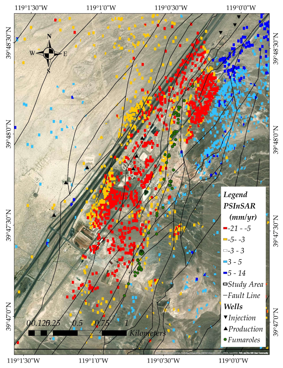 |
| Time | (a) 2013 May–2014 May | (b) 2011–2015 | (c) 2016 July–2017 Aug | (d) 2017 Dec–2019 Dec |
| Range | −15–15 mm/yr | −13–13 mm/yr | −25–25 mm/yr | −21–14 mm/yr |
| Stdv. | 3.3 mm/yr | 2.2 mm/yr | ||
| Ave. | − 9.9 mm/yr | − 6.4 mm/yr | ||
| Ref. | [25] | [25] | [29] | PSI analysis with 70 images |
| Year/Months | January | February | April | May | June | July | August | October |
|---|---|---|---|---|---|---|---|---|
| 2018 | 03.01.18 | 20.02.18 | 09.04.18 | 15.05.18 | 08.06.18 | 02.07.18 | 31.08.18 | 18.10.18 |
| 2019 | 10.01.19 22.01.19 | 15.06.19 27.06.19 | 02.08.19 | 25.10.19 |
Publisher’s Note: MDPI stays neutral with regard to jurisdictional claims in published maps and institutional affiliations. |
© 2021 by the authors. Licensee MDPI, Basel, Switzerland. This article is an open access article distributed under the terms and conditions of the Creative Commons Attribution (CC BY) license (http://creativecommons.org/licenses/by/4.0/).
Share and Cite
Cavur, M.; Moraga, J.; Duzgun, H.S.; Soydan, H.; Jin, G. Displacement Analysis of Geothermal Field Based on PSInSAR And SOM Clustering Algorithms A Case Study of Brady Field, Nevada—USA. Remote Sens. 2021, 13, 349. https://doi.org/10.3390/rs13030349
Cavur M, Moraga J, Duzgun HS, Soydan H, Jin G. Displacement Analysis of Geothermal Field Based on PSInSAR And SOM Clustering Algorithms A Case Study of Brady Field, Nevada—USA. Remote Sensing. 2021; 13(3):349. https://doi.org/10.3390/rs13030349
Chicago/Turabian StyleCavur, Mahmut, Jaime Moraga, H. Sebnem Duzgun, Hilal Soydan, and Ge Jin. 2021. "Displacement Analysis of Geothermal Field Based on PSInSAR And SOM Clustering Algorithms A Case Study of Brady Field, Nevada—USA" Remote Sensing 13, no. 3: 349. https://doi.org/10.3390/rs13030349