
A Satellite-Based Land Use Regression Model of Ambient NO2 with High Spatial Resolution in a Chinese City


Abstract
:1. Introduction
2. Materials and Methods
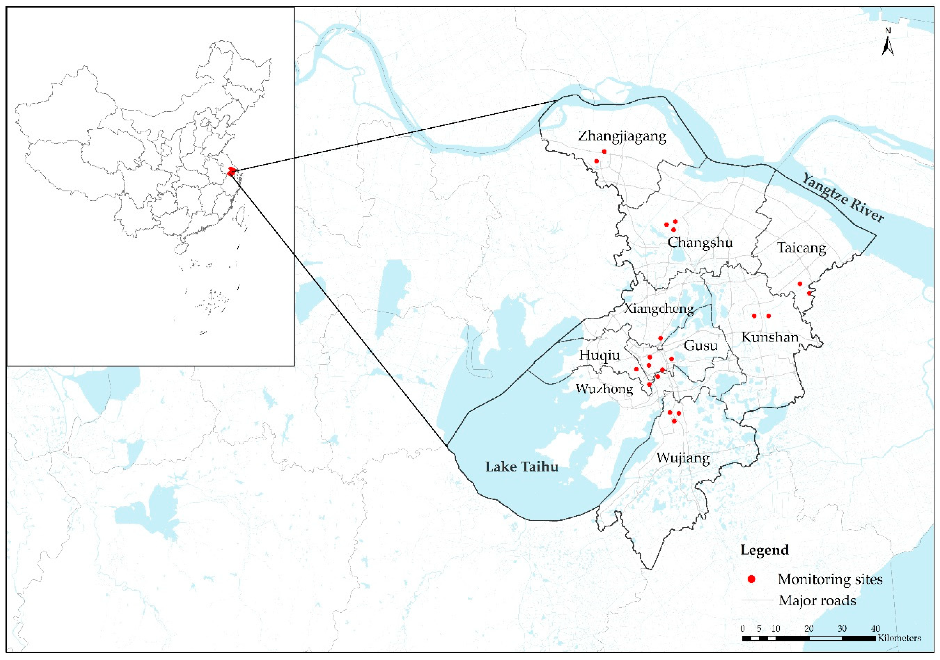
2.1. Study Area
2.2. Data
2.2.1. Monitoring Data
2.2.2. Satellite Data
2.2.3. Other Predictors
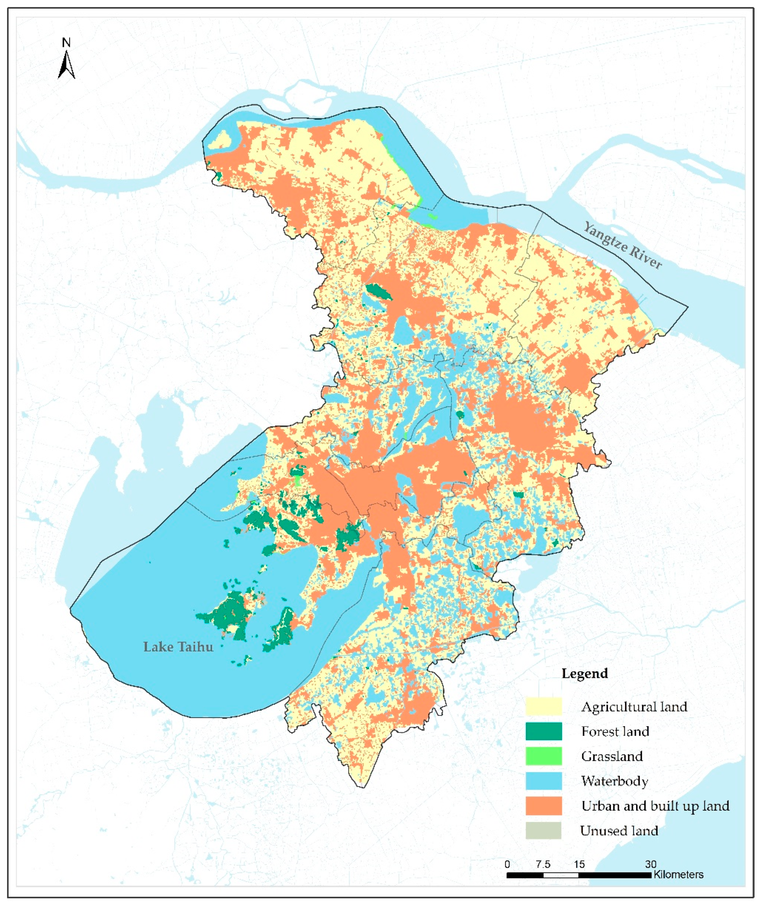
Land Use Parameters
Road Network
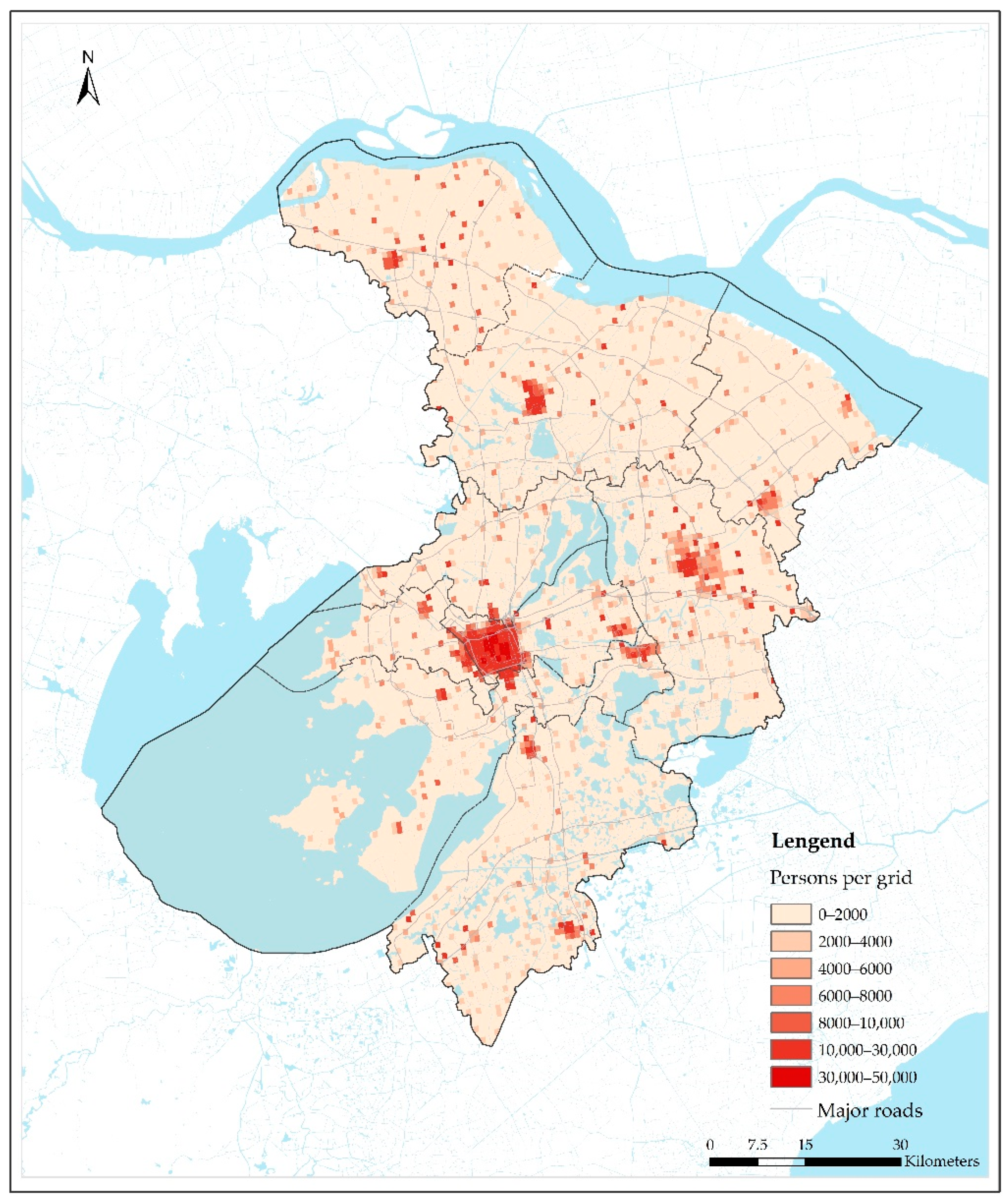
Population Density
NOx Emissions
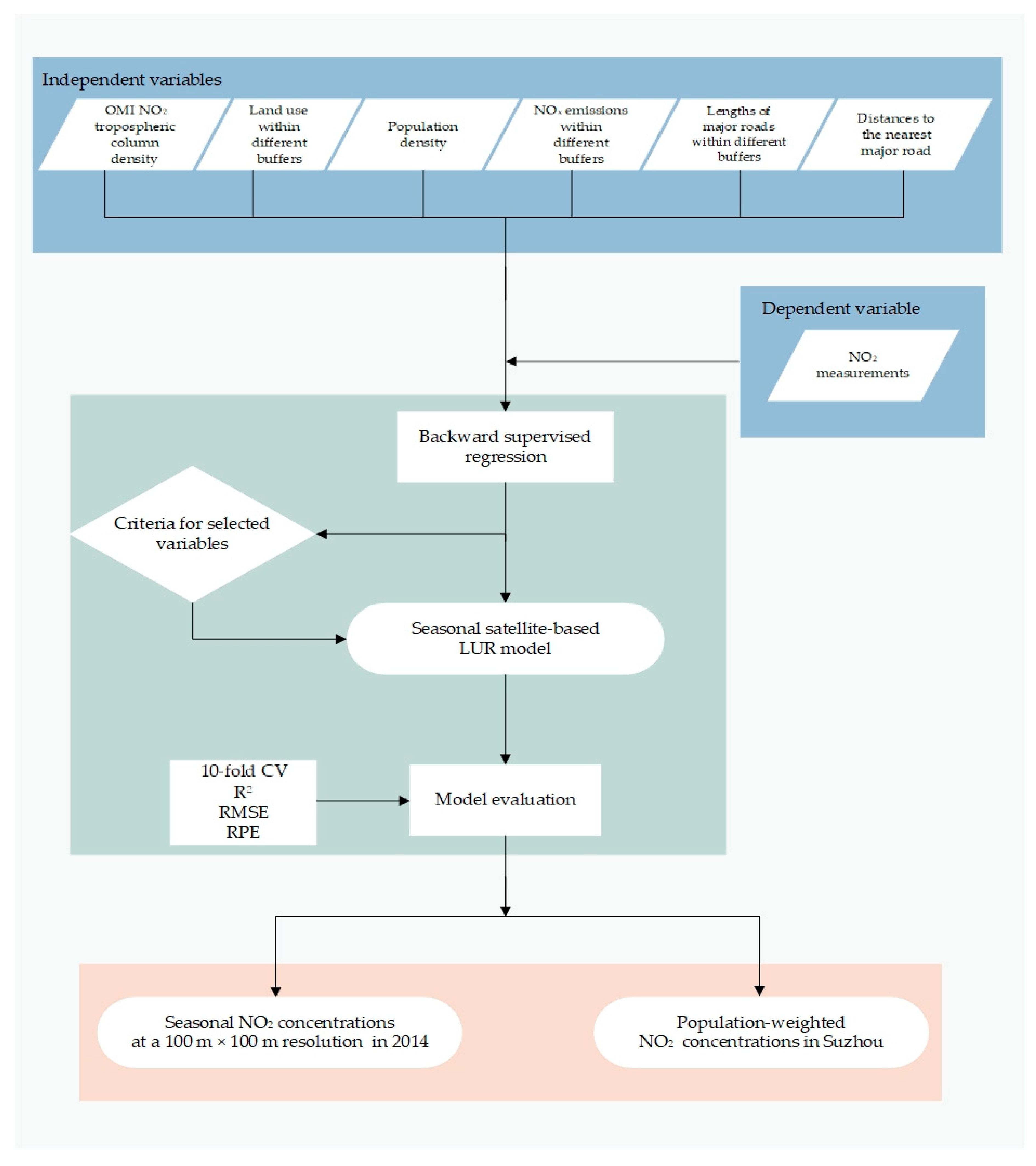
2.3. Model Development and Evaluation
3. Results
3.1. Descriptive Statistics Analyses
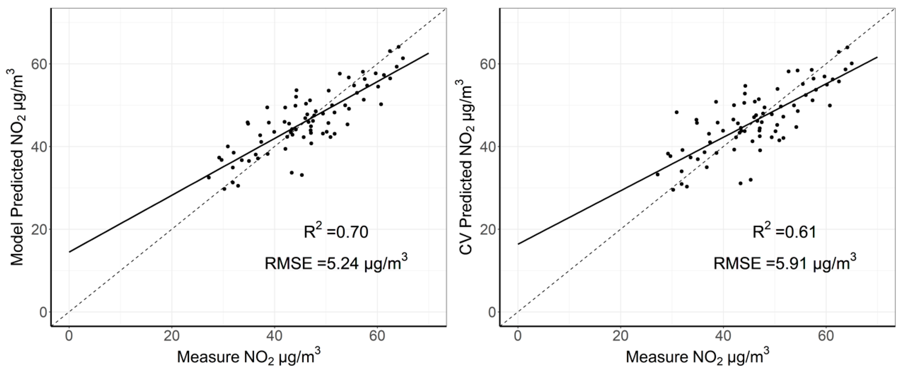
3.2. Model Development and Evaluation
3.3. Spatiotemporal Trends of Predicting NO2 Concentrations
4. Discussion
5. Conclusions
Author Contributions
Funding
Institutional Review Board Statement
Informed Consent Statement
Data Availability Statement
Acknowledgments
Conflicts of Interest
References
- Casquero-Vera, J.A.; Lyamani, H.; Titos, G.; Borras, E.; Olmo, F.J.; Alados-Arboledas, L. Impact of primary NO2 emissions at different urban sites exceeding the European NO2 standard limit. Sci. Total Environ. 2019, 646, 1117–1125. [Google Scholar] [CrossRef]
- Anttila, P.; Tuovinen, J.-P.; Niemi, J.V. Primary NO2 emissions and their role in the development of NO2 concentrations in a traffic environment. Atmos. Environ. 2011, 45, 986–992. [Google Scholar] [CrossRef]
- Jerrett, M.; Burnett, R.T.; Beckerman, B.S.; Turner, M.C.; Krewski, D.; Thurston, G.; Martin, R.V.; van Donkelaar, A.; Hughes, E.; Shi, Y.; et al. Spatial analysis of air pollution and mortality in California. Am. J. Respir. Crit. Care Med. 2013, 188, 593–599. [Google Scholar] [CrossRef] [PubMed]
- Chen, R.; Yin, P.; Meng, X.; Wang, L.; Liu, C.; Niu, Y.; Lin, Z.; Liu, Y.; Liu, J.; Qi, J.; et al. Associations Between Ambient Nitrogen Dioxide and Daily Cause-specific Mortality: Evidence from 272 Chinese Cities. Epidemiology 2018, 29, 482–489. [Google Scholar] [CrossRef] [PubMed]
- WHO Regional Office for Europe. Review of Evidence on Health Aspects of Air Pollution—REVIHAAP Project: Technical Report; WHO Regional Office for Europe: Copenhagen, Denmark, 2013. Available online: https://www.ncbi.nlm.nih.gov/books/NBK361805/ (accessed on 13 November 2020).
- Beelen, R.; Hoek, G.; Vienneau, D.; Eeftens, M.; Dimakopoulou, K.; Pedeli, X.; Tsai, M.-Y.; Künzli, N.; Schikowski, T.; Marcon, A.; et al. Development of NO2 and NOx land use regression models for estimating air pollution exposure in 36 study areas in Europe—The ESCAPE project. Atmos. Environ. 2013, 72, 10–23. [Google Scholar] [CrossRef]
- Son, J.Y.; Bell, M.L.; Lee, J.T. Individual exposure to air pollution and lung function in Korea: Spatial analysis using multiple exposure approaches. Environ. Res. 2010, 110, 739–749. [Google Scholar] [CrossRef] [PubMed]
- Karner, A.A.; Eisinger, D.S.; Niemeier, D.A. Near-roadway air quality: Synthesizing the findings from real-world data. Environ. Sci. Technol. 2010, 44, 5334–5344. [Google Scholar] [CrossRef] [PubMed]
- Cyrys, J.; Eeftens, M.; Heinrich, J.; Ampe, C.; Armengaud, A.; Beelen, R.; Bellander, T.; Beregszaszi, T.; Birk, M.; Cesaroni, G.; et al. Variation of NO2 and NOx concentrations between and within 36 European study areas: Results from the ESCAPE study. Atmos. Environ. 2012, 62, 374–390. [Google Scholar] [CrossRef]
- Lee, J.H.; Wu, C.F.; Hoek, G.; de Hoogh, K.; Beelen, R.; Brunekreef, B.; Chan, C.C. Land use regression models for estimating individual NOx and NO2 exposures in a metropolis with a high density of traffic roads and population. Sci. Total Environ. 2014, 472, 1163–1171. [Google Scholar] [CrossRef]
- Crouse, D.L.; Peters, P.A.; Villeneuve, P.J.; Proux, M.O.; Shin, H.H.; Goldberg, M.S.; Johnson, M.; Wheeler, A.J.; Allen, R.W.; Atari, D.O.; et al. Within- and between-city contrasts in nitrogen dioxide and mortality in 10 Canadian cities; a subset of the Canadian Census Health and Environment Cohort (CanCHEC). J. Expo. Sci. Environ. Epidemiol. 2015, 25, 482–489. [Google Scholar] [CrossRef] [Green Version]
- de Hoogh, K.; Gulliver, J.; Donkelaar, A.v.; Martin, R.V.; Marshall, J.D.; Bechle, M.J.; Cesaroni, G.; Pradas, M.C.; Dedele, A.; Eeftens, M.; et al. Development of West-European PM2.5 and NO2 land use regression models incorporating satellite-derived and chemical transport modelling data. Environ. Res. 2016, 151, 1–10. [Google Scholar] [CrossRef] [PubMed] [Green Version]
- Fischer, P.H.; Marra, M.; Ameling, C.B.; Hoek, G.; Beelen, R.; de Hoogh, K.; Breugelmans, O.; Kruize, H.; Janssen, N.A.; Houthuijs, D. Air Pollution and Mortality in Seven Million Adults: The Dutch Environmental Longitudinal Study (DUELS). Environ. Health Perspect. 2015, 123, 697–704. [Google Scholar] [CrossRef] [PubMed] [Green Version]
- Foraster, M.; Basagana, X.; Aguilera, I.; Rivera, M.; Agis, D.; Bouso, L.; Deltell, A.; Marrugat, J.; Ramos, R.; Sunyer, J.; et al. Association of long-term exposure to traffic-related air pollution with blood pressure and hypertension in an adult population-based cohort in Spain (the REGICOR study). Environ. Health Perspect. 2014, 122, 404–411. [Google Scholar] [CrossRef] [PubMed]
- Ohlwein, S.; Klumper, C.; Vossoughi, M.; Sugiri, D.; Stolz, S.; Vierkotter, A.; Schikowski, T.; Kara, K.; Germing, A.; Quass, U.; et al. Air pollution and diastolic function in elderly women—Results from the SALIA study cohort. Int. J. Hyg. Environ. Health 2016, 219, 356–363. [Google Scholar] [CrossRef] [PubMed]
- Chen, L.; Wang, Y.; Li, P.; Ji, Y.; Kong, S.; Li, Z.; Bai, Z. A land use regression model incorporating data on industrial point source pollution. J. Environ. Sci. 2012, 24, 1251–1258. [Google Scholar] [CrossRef]
- Meng, X.; Chen, L.; Cai, J.; Zou, B.; Wu, C.-F.; Fu, Q.; Zhang, Y.; Liu, Y.; Kan, H. A land use regression model for estimating the NO2 concentration in Shanghai, China. Environ. Res. 2015, 137, 308–315. [Google Scholar] [CrossRef]
- Xu, G.; Jiao, L.M.; Zhao, S.L.; Yuan, M.; Li, X.M.; Han, Y.Y.; Zhang, B.; Dong, T. Examining the Impacts of Land Use on Air Quality from a Spatio-Temporal Perspective in Wuhan, China. Atmosphere 2016, 7, 62. [Google Scholar] [CrossRef] [Green Version]
- Bechle, M.J.; Millet, D.B.; Marshall, J.D. National Spatiotemporal Exposure Surface for NO2: Monthly Scaling of a Satellite-Derived Land-Use Regression, 2000–2010. Environ. Sci. Technol. 2015, 49, 12297–12305. [Google Scholar] [CrossRef]
- Larkin, A.; Geddes, J.A.; Martin, R.V.; Xiao, Q.; Liu, Y.; Marshall, J.D.; Brauer, M.; Hystad, P. Global Land Use Regression Model for Nitrogen Dioxide Air Pollution. Environ. Sci. Technol. 2017, 51, 6957–6964. [Google Scholar] [CrossRef]
- Yang, X.; Zheng, Y.; Geng, G.; Liu, H.; Man, H.; Lv, Z.; He, K.; de Hoogh, K. Development of PM2.5 and NO2 models in a LUR framework incorporating satellite remote sensing and air quality model data in Pearl River Delta region, China. Environ. Pollut. 2017, 226, 143–153. [Google Scholar] [CrossRef]
- Vienneau, D.; de Hoogh, K.; Bechle, M.J.; Beelen, R.; van Donkelaar, A.; Martin, R.V.; Millet, D.B.; Hoek, G.; Marshall, J.D. Western European land use regression incorporating satellite- and ground-based measurements of NO2 and PM10. Environ. Sci. Technol. 2013, 47, 13555–13564. [Google Scholar] [CrossRef] [PubMed]
- Meng, X.; Fu, Q.; Ma, Z.; Chen, L.; Zou, B.; Zhang, Y.; Xue, W.; Wang, J.; Wang, D.; Kan, H.; et al. Estimating ground-level PM10 in a Chinese city by combining satellite data, meteorological information and a land use regression model. Environ. Pollut. 2016, 208, 177–184. [Google Scholar] [CrossRef] [PubMed]
- Ma, X.; Jia, H.; Sha, T.; An, J.; Tian, R. Spatial and seasonal characteristics of particulate matter and gaseous pollution in China: Implications for control policy. Environ. Pollut. 2019, 248, 421–428. [Google Scholar] [CrossRef] [PubMed]
- Zhang, Z.; Wang, J.; Hart, J.E.; Laden, F.; Zhao, C.; Li, T.; Zheng, P.; Li, D.; Ye, Z.; Chen, K. National scale spatiotemporal land-use regression model for PM2.5, PM10 and NO2 concentration in China. Atmos. Environ. 2018, 192, 48–54. [Google Scholar] [CrossRef]
- Hoek, G.; Eeftens, M.; Beelen, R.; Fischer, P.; Brunekreef, B.; Boersma, K.F.; Veefkind, P. Satellite NO2 data improve national land use regression models for ambient NO2 in a small densely populated country. Atmos. Environ. 2015, 105, 173–180. [Google Scholar] [CrossRef]
- Novotny, E.V.; Bechle, M.J.; Millet, D.B.; Marshall, J.D. National Satellite-Based Land-Use Regression: NO2 in the United States. Environ. Sci. Technol. 2011, 45, 4407–4414. [Google Scholar] [CrossRef]
- Zhan, Y.; Luo, Y.; Deng, X.; Zhang, K.; Zhang, M.; Grieneisen, M.L.; Di, B. Satellite-Based Estimates of Daily NO2 Exposure in China Using Hybrid Random Forest and Spatiotemporal Kriging Model. Environ. Sci. Technol. 2018, 52, 4180–4189. [Google Scholar] [CrossRef]
- Knibbs, L.D.; Coorey, C.P.; Bechle, M.J.; Marshall, J.D.; Hewson, M.G.; Jalaludin, B.; Morgan, G.G.; Barnett, A.G. Long-term nitrogen dioxide exposure assessment using back-extrapolation of satellite-based land-use regression models for Australia. Environ. Res. 2018, 163, 16–25. [Google Scholar] [CrossRef]
- Knibbs, L.D.; Hewson, M.G.; Bechle, M.J.; Marshall, J.D.; Barnett, A.G. A national satellite-based land-use regression model for air pollution exposure assessment in Australia. Environ. Res. 2014, 135, 204–211. [Google Scholar] [CrossRef] [Green Version]
- Xu, H.; Bechle, M.J.; Wang, M.; Szpiro, A.A.; Vedal, S.; Bai, Y.; Marshall, J.D. National PM2.5 and NO2 exposure models for China based on land use regression, satellite measurements, and universal kriging. Sci. Total Environ. 2019, 655, 423–433. [Google Scholar] [CrossRef] [Green Version]
- McPeters, R.D.; Frith, S.; Labow, G.J. OMI total column ozone: Extending the long-term data record. Atmos. Meas. Tech. 2015, 8, 4845–4850. [Google Scholar] [CrossRef] [Green Version]
- Xiao, Q.; Chang, H.H.; Geng, G.; Liu, Y. An Ensemble Machine-Learning Model to Predict Historical PM2.5 Concentrations in China from Satellite Data. Environ. Sci. Technol. 2018, 52, 13260–13269. [Google Scholar] [CrossRef] [PubMed]
- Chen, Z.; Chen, J.; Collins, R.; Guo, Y.; Peto, R.; Wu, F.; Li, L. China Kadoorie Biobank of 0.5 million people: Survey methods, baseline characteristics and long-term follow-up. Int. J. Epidemiol. 2011, 40, 1652–1666. [Google Scholar] [CrossRef] [PubMed] [Green Version]
- Levelt, P.F.; van den Oord, G.H.J.; Dobber, M.R.; Malkki, A.; Huib, V.; Johan de, V.; Stammes, P.; Lundell, J.O.V.; Saari, H. The ozone monitoring instrument. IEEE Trans. Geosci. Remote Sens. 2006, 44, 1093–1101. [Google Scholar] [CrossRef]
- Hoek, G.; Beelen, R.; de Hoogh, K.; Vienneau, D.; Gulliver, J.; Fischer, P.; Briggs, D. A review of land-use regression models to assess spatial variation of outdoor air pollution. Atmos. Environ. 2008, 42, 7561–7578. [Google Scholar] [CrossRef]
- Ma, Z.; Hu, X.; Sayer, A.M.; Levy, R.; Zhang, Q.; Xue, Y.; Tong, S.; Bi, J.; Huang, L.; Liu, Y. Satellite-Based Spatiotemporal Trends in PM2.5 Concentrations: China, 2004–2013. Environ. Health Perspect. 2016, 124, 184–192. [Google Scholar] [CrossRef] [Green Version]
- Saucy, A.; Roosli, M.; Kunzli, N.; Tsai, M.-Y.; Sieber, C.; Olaniyan, T.; Baatjies, R.; Jeebhay, M.; Davey, M.; Fluckiger, B.; et al. Land Use Regression Modelling of Outdoor NO2 and PM2.5 Concentrations in Three Low Income Areas in the Western Cape Province, South Africa. Int. J. Environ. Res. Public Health 2018, 15, 1452. [Google Scholar] [CrossRef] [Green Version]
- de Hoogh, K.; Chen, J.; Gulliver, J.; Hoffmann, B.; Hertel, O.; Ketzel, M.; Bauwelinck, M.; van Donkelaar, A.; Hvidtfeldt, U.A.; Katsouyanni, K.; et al. Spatial PM2.5, NO2, O3 and BC models for Western Europe—Evaluation of spatiotemporal stability. Environ. Int. 2018, 120, 81–92. [Google Scholar] [CrossRef]
- Chen, Z.Y.; Zhang, R.; Zhang, T.H.; Ou, C.Q.; Guo, Y. A kriging-calibrated machine learning method for estimating daily ground-level NO2 in mainland China. Sci. Total Environ. 2019, 690, 556–564. [Google Scholar] [CrossRef]
- Di, Q.; Amini, H.; Shi, L.; Kloog, I.; Silvern, R.; Kelly, J.; Sabath, M.B.; Choirat, C.; Koutrakis, P.; Lyapustin, A.; et al. Assessing NO2 Concentration and Model Uncertainty with High Spatiotemporal Resolution across the Contiguous United States Using Ensemble Model Averaging. Environ. Sci. Technol. 2020, 54, 1372–1384. [Google Scholar] [CrossRef]
- Li, T.; Wang, Y.; Yuan, Q. Remote Sensing Estimation of Regional NO2 via Space-Time Neural Networks. Remote Sens. 2020, 12, 2514. [Google Scholar] [CrossRef]
- Zhang, T.; He, W.; Zheng, H.; Cui, Y.; Song, H.; Fu, S. Satellite-based ground PM2.5 estimation using a gradient boosting decision tree. Chemosphere 2020, 128801. [Google Scholar] [CrossRef] [PubMed]
- Wang, H.; Miao, Q.; Shen, L.; Yang, Q.; Wu, Y.; Wei, H. Air pollutant variations in Suzhou during the 2019 novel coronavirus (COVID-19) lockdown of 2020: High time-resolution measurements of aerosol chemical compositions and source apportionment. Environ. Pollut. 2020, 271, 116298. [Google Scholar] [CrossRef] [PubMed]
- Kuerban, M.; Waili, Y.; Fan, F.; Liu, Y.; Qin, W.; Dore, A.J.; Peng, J.; Xu, W.; Zhang, F. Spatio-temporal patterns of air pollution in China from 2015 to 2018 and implications for health risks. Environ. Pollut. 2020, 258, 113659. [Google Scholar] [CrossRef] [PubMed]
- Ye, S.; Ma, T.; Duan, F.; Li, H.; He, K.; Xia, J.; Yang, S.; Zhu, L.; Ma, Y.; Huang, T.; et al. Characteristics and formation mechanisms of winter haze in Changzhou, a highly polluted industrial city in the Yangtze River Delta, China. Environ. Pollut. 2019, 253, 377–383. [Google Scholar] [CrossRef]
- Shen, Y.; Jiang, F.; Feng, S.; Zheng, Y.; Cai, Z.; Lyu, X. Impact of weather and emission changes on NO2 concentrations in China during 2014–2019. Environ. Pollut. 2021, 269, 116163. [Google Scholar] [CrossRef]
- Shen, G.; Ru, M.; Du, W.; Zhu, X.; Zhong, Q.; Chen, Y.; Shen, H.; Yun, X.; Meng, W.; Liu, J.; et al. Impacts of air pollutants from rural Chinese households under the rapid residential energy transition. Nat. Commun. 2019, 10, 3405. [Google Scholar] [CrossRef] [Green Version]


| Variables | β | SE | p Value |
|---|---|---|---|
| Intercept | 33.57 | 5.13 | <0.001 |
| NO2 tropospheric column density | 0.85 | 0.11 | <0.001 |
| Population density | 0.00016 | 0.0001 | 0.043 |
| Log_distance | 2.92 | 1.38 | 0.038 |
| Non-power emissions within 10 km buffer zone | 0.0001 | 0.00003 | 0.002 |
| Variables | β | SE | p Value | IQR × β 1 |
|---|---|---|---|---|
| Intercept | 39.617 | 7.348 | <0.001 | |
| NO2 tropospheric column density | 0.618 | 0.293 | 0.039 | 4.389 |
| Population density | 0.00016 | 0.0001 | 0.029 | 1.976 |
| Log_distance | 3.240 | 1.272 | 0.013 | 1.546 |
| Non-power emissions within 10-km buffer zone | 0.0001 | 0.00003 | <0.001 | 4.792 |
| Parameter | Annual | Spring | Summer | Autumn | Winter |
|---|---|---|---|---|---|
| Population-weighted concentration (μg/m3) | 44.94 | 46.33 | 35.64 | 46.59 | 51.21 |
| Proportion (%) * | 84 | 92 | 22 | 96 | 99 |
Publisher’s Note: MDPI stays neutral with regard to jurisdictional claims in published maps and institutional affiliations. |
© 2021 by the authors. Licensee MDPI, Basel, Switzerland. This article is an open access article distributed under the terms and conditions of the Creative Commons Attribution (CC BY) license (http://creativecommons.org/licenses/by/4.0/).
Share and Cite
Zhang, L.; Yang, C.; Xiao, Q.; Geng, G.; Cai, J.; Chen, R.; Meng, X.; Kan, H. A Satellite-Based Land Use Regression Model of Ambient NO2 with High Spatial Resolution in a Chinese City. Remote Sens. 2021, 13, 397. https://doi.org/10.3390/rs13030397
Zhang L, Yang C, Xiao Q, Geng G, Cai J, Chen R, Meng X, Kan H. A Satellite-Based Land Use Regression Model of Ambient NO2 with High Spatial Resolution in a Chinese City. Remote Sensing. 2021; 13(3):397. https://doi.org/10.3390/rs13030397
Chicago/Turabian StyleZhang, Lina, Changyuan Yang, Qingyang Xiao, Guannan Geng, Jing Cai, Renjie Chen, Xia Meng, and Haidong Kan. 2021. "A Satellite-Based Land Use Regression Model of Ambient NO2 with High Spatial Resolution in a Chinese City" Remote Sensing 13, no. 3: 397. https://doi.org/10.3390/rs13030397