
A New Method to Predict Gully Head Erosion in the Loess Plateau of China Based on SBAS-InSAR

Abstract
:
1. Introduction
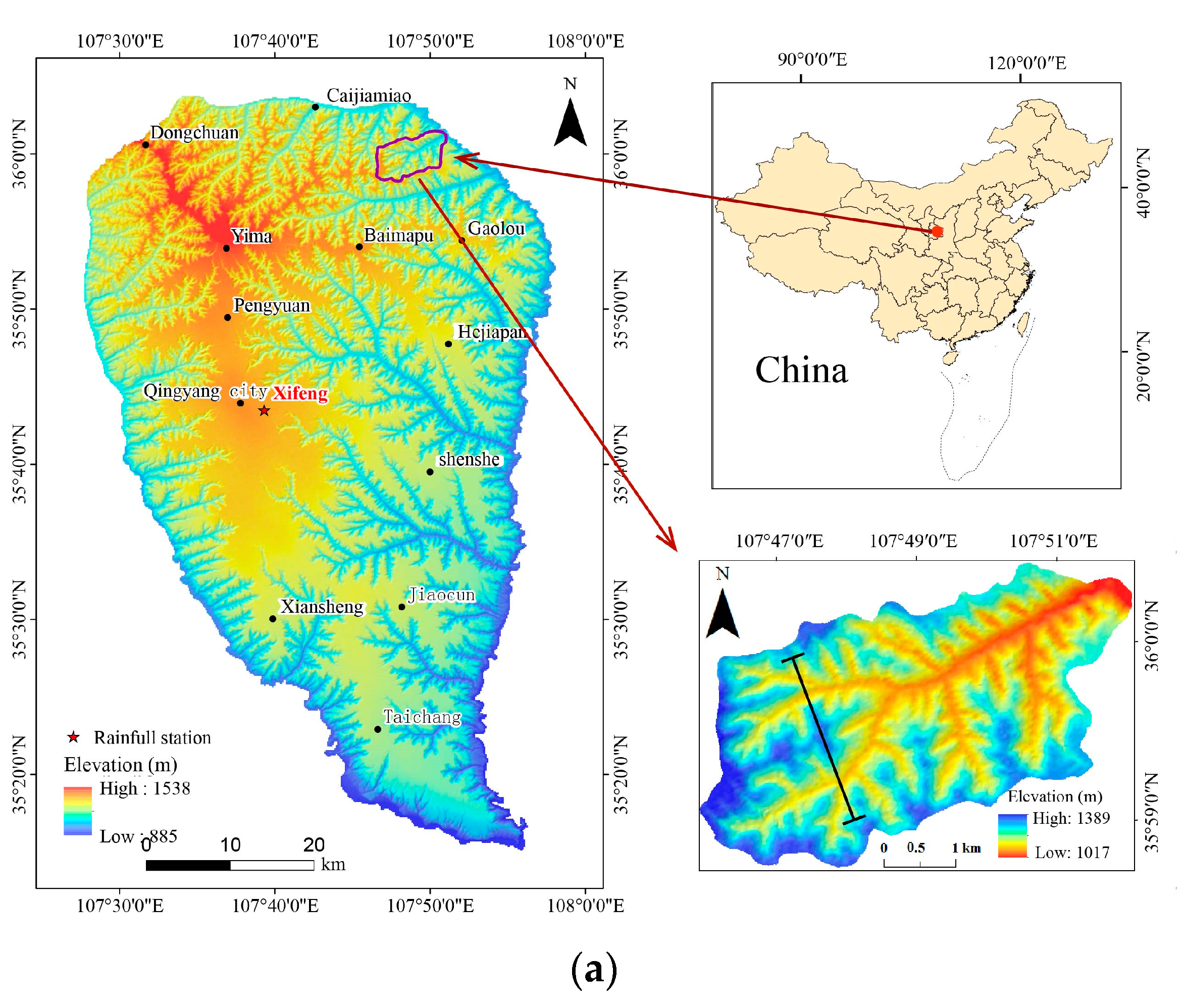
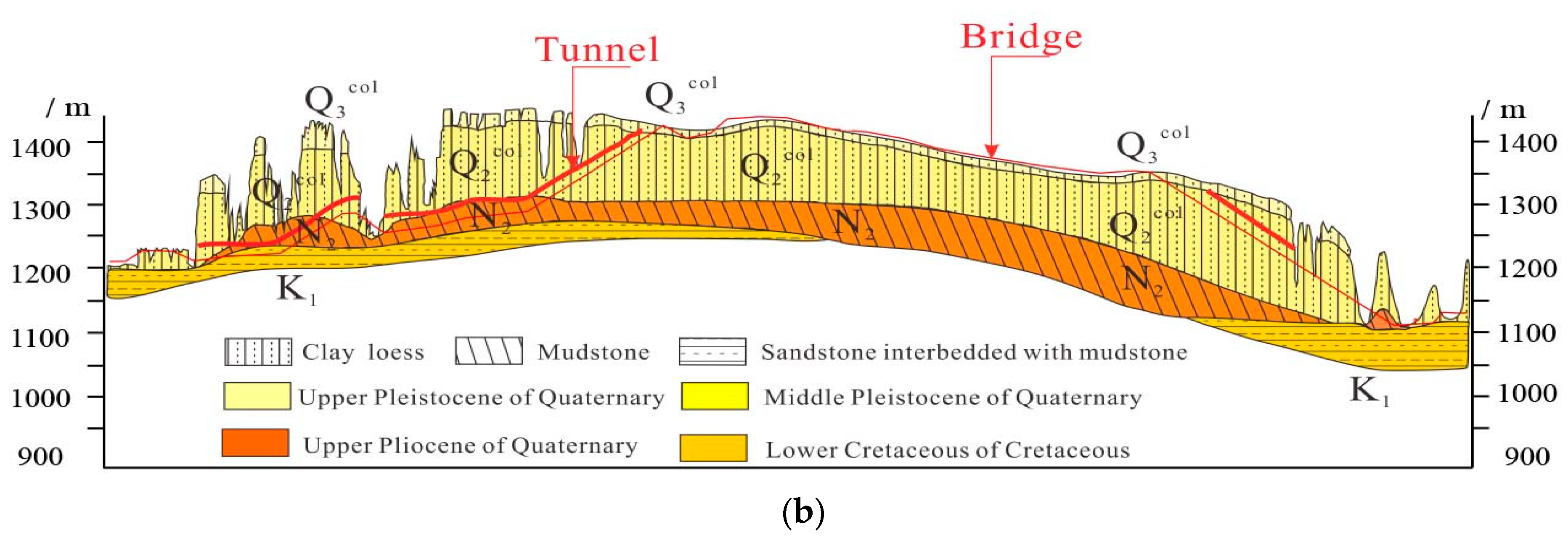
2. Research Area
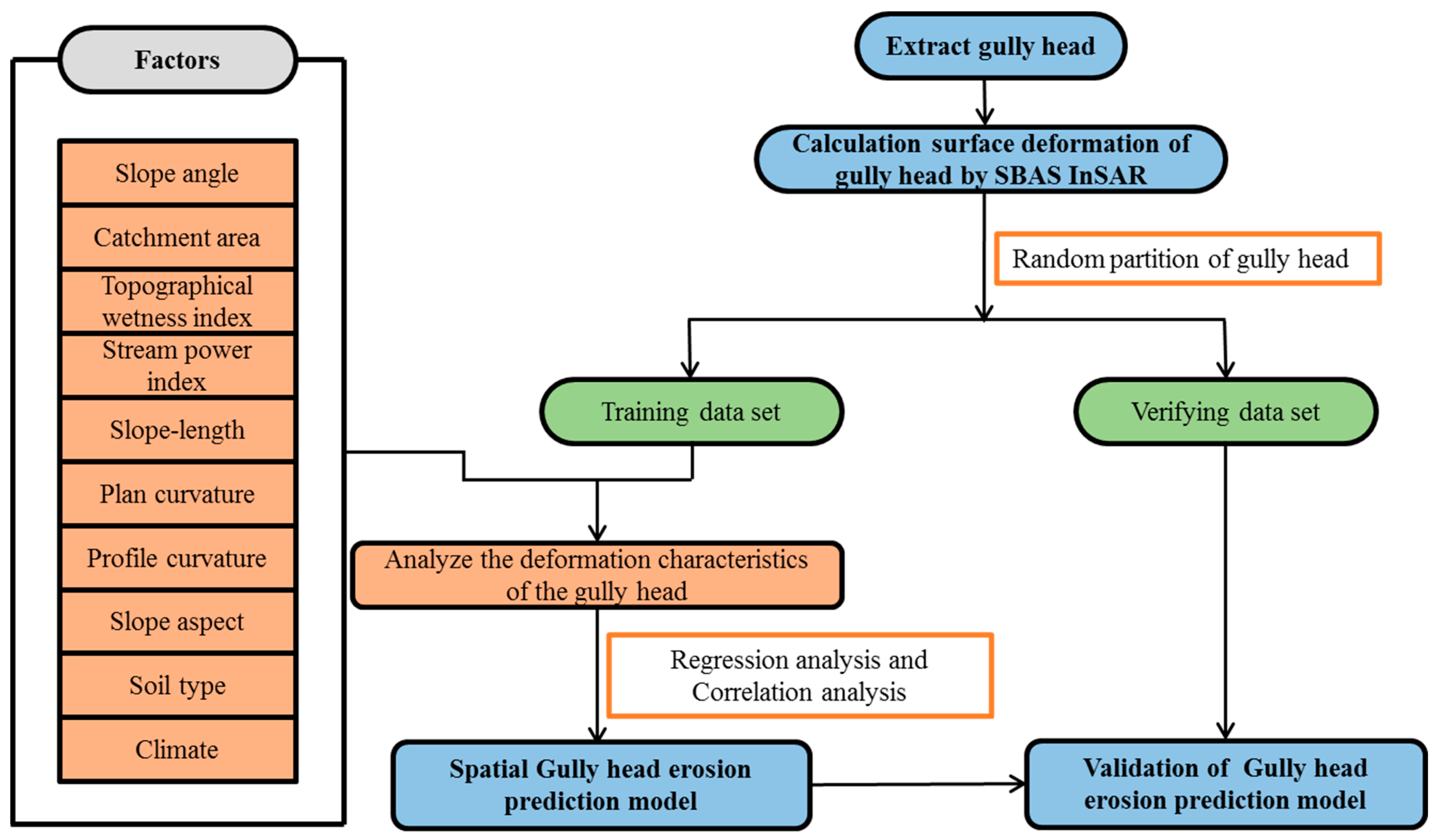
3. Materials and Methods
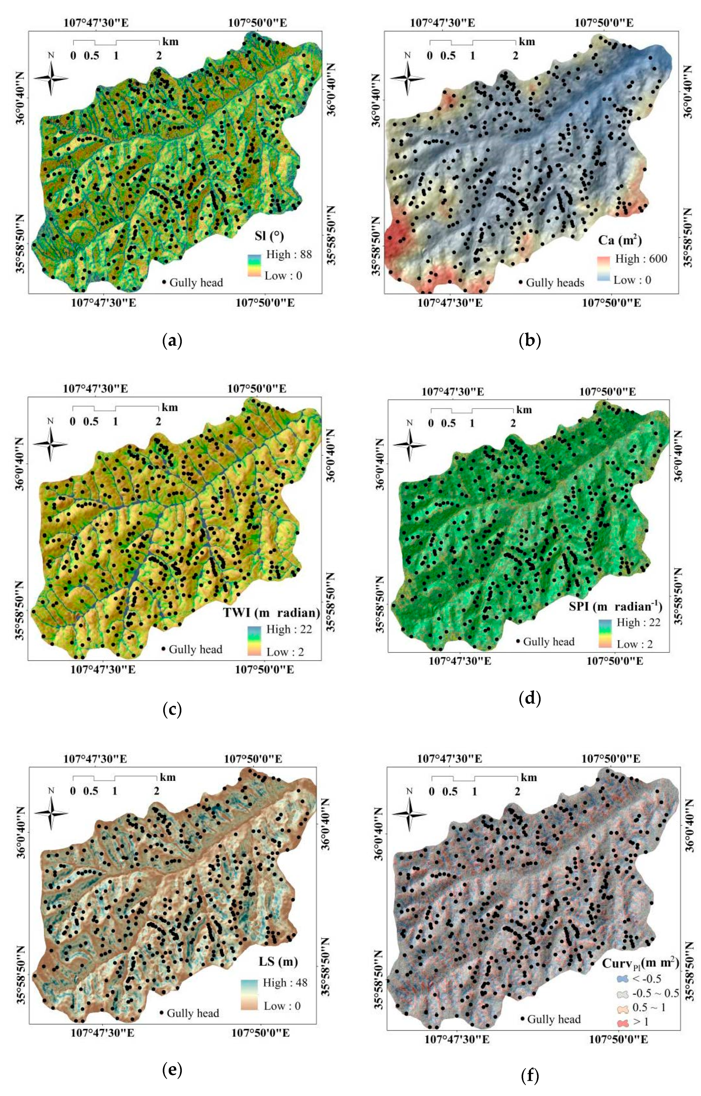
3.1. Terrain Attributes from a DEM
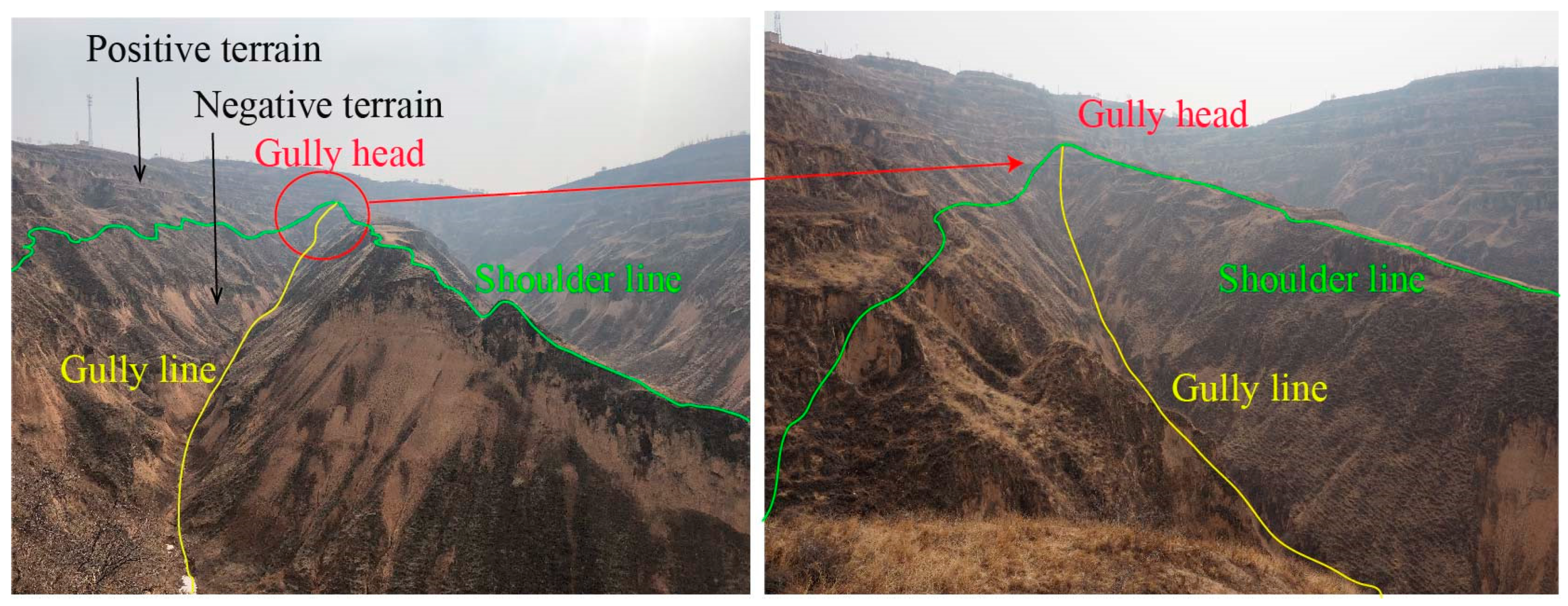
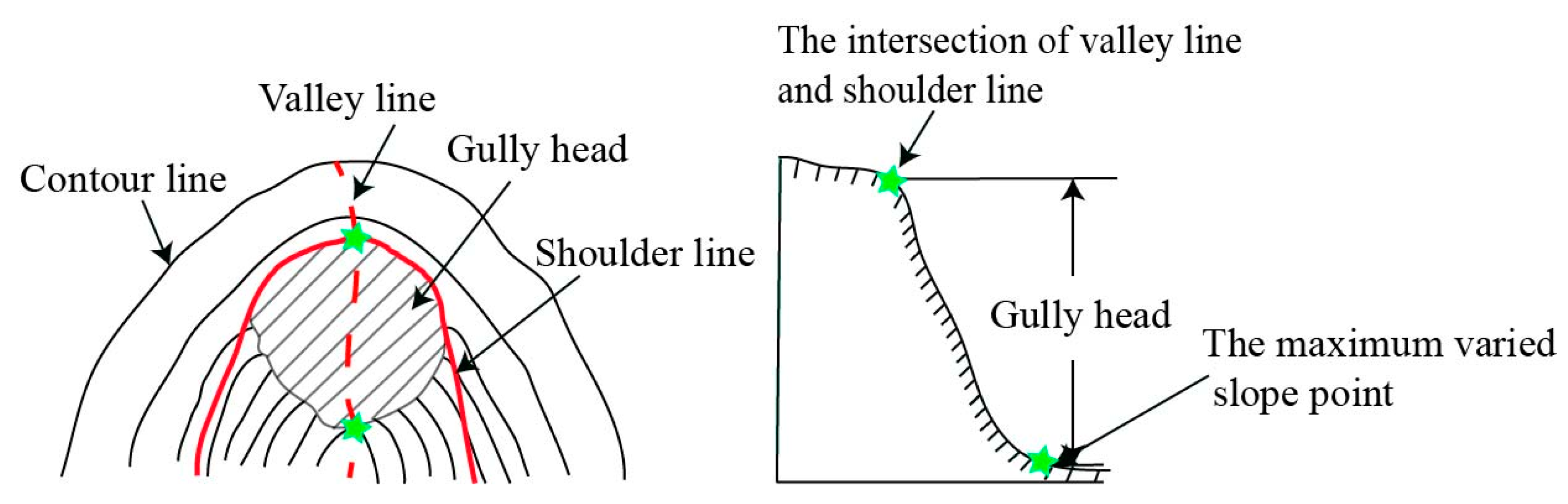
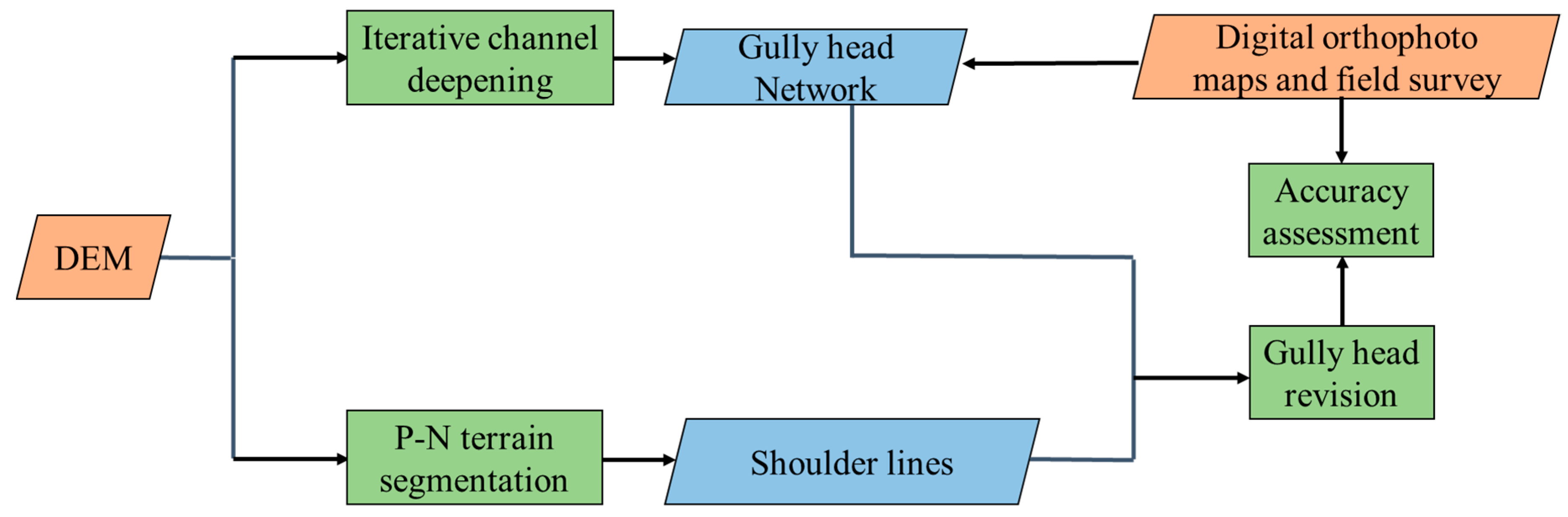
3.2. Gully Head Detection with a DEM
3.3. Monitoring the Gully Head Erosion with SBAS-InSAR
3.4. Evaluating the Gully Head Erosion Rate (GHER)
3.5. Evaluating the Validity and Efficiency of the Model
4. Results
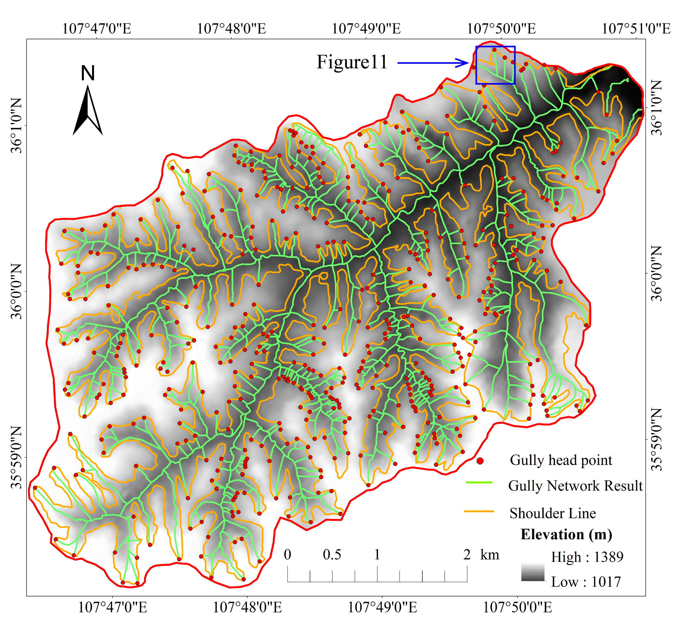
4.1. Locating of the Gully Heads
4.2. Gully Head Erosion Rates
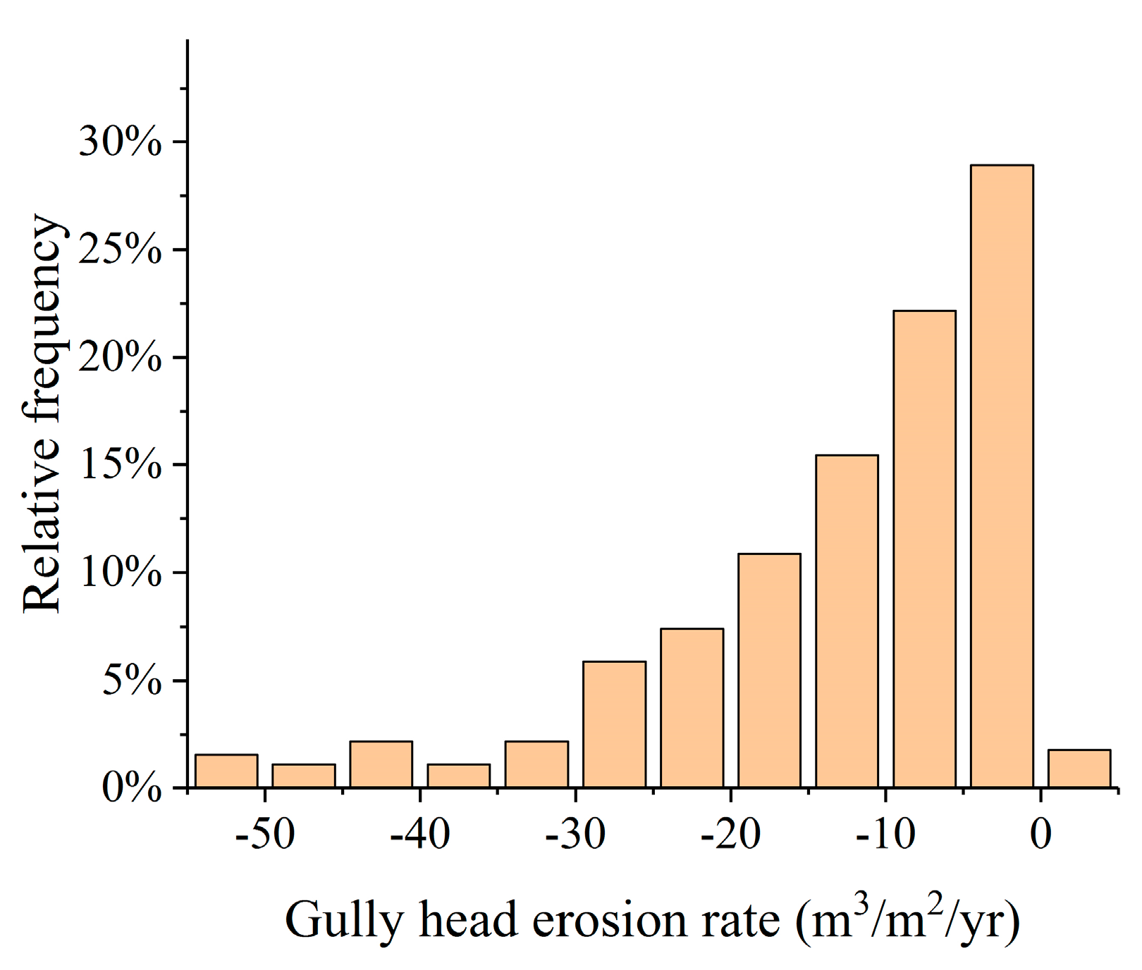
4.2.1. SBAS-InSAR Results
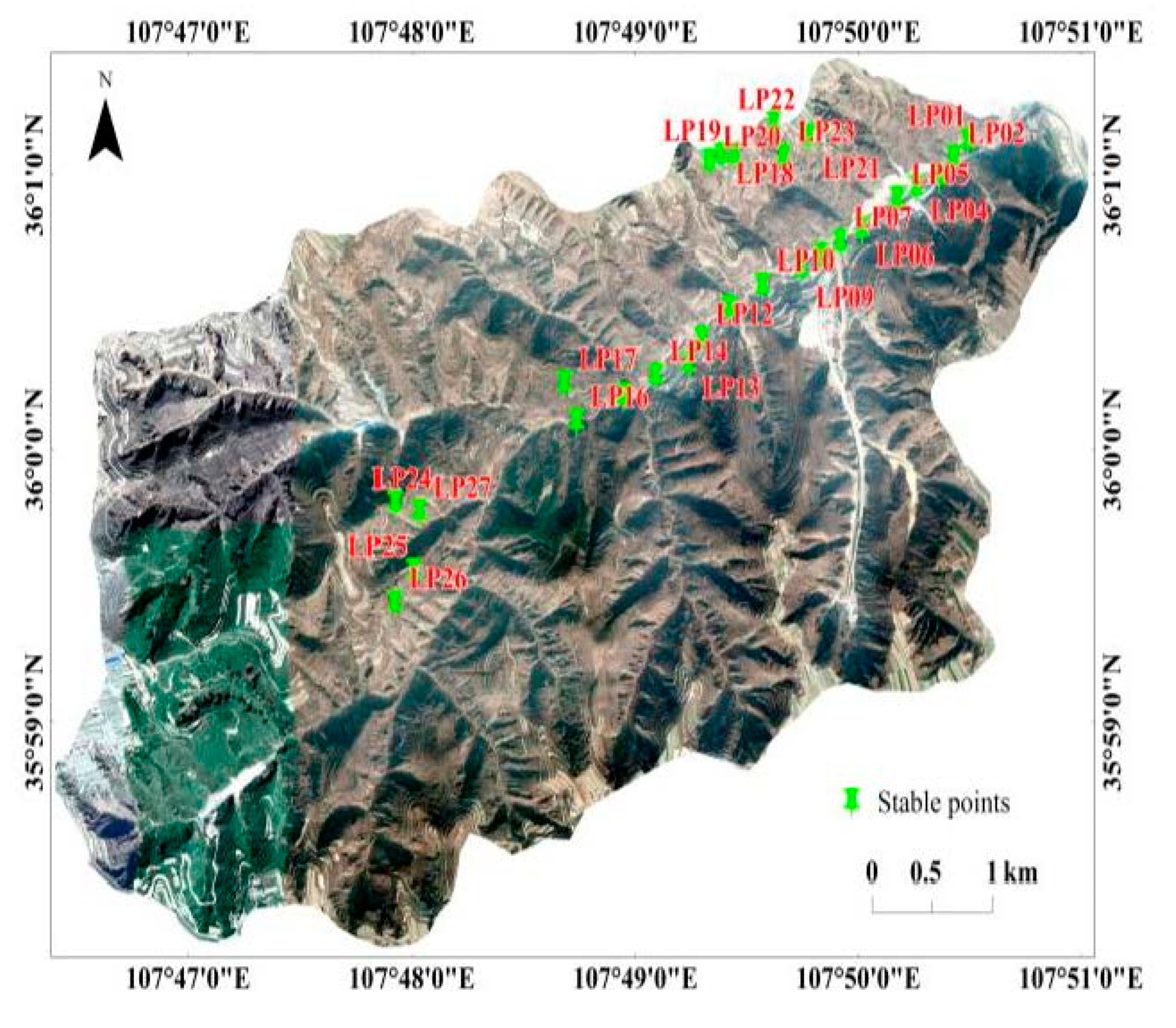
4.2.2. Accuracy Assessment of the SBAS-InSAR Results
4.3. Spatial Factors That Influence the Gully Head Erosion Rate
4.3.1. Precipitation
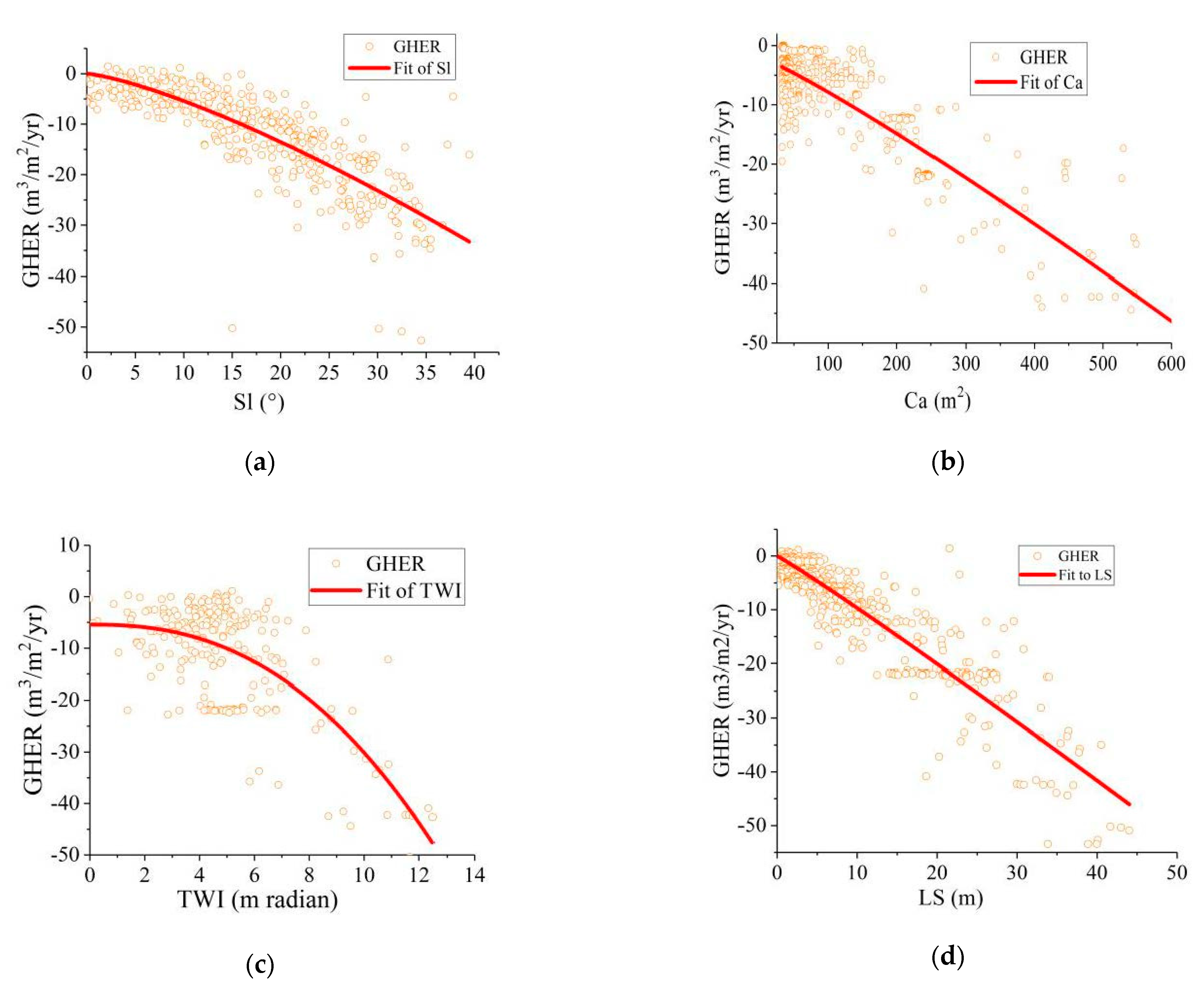
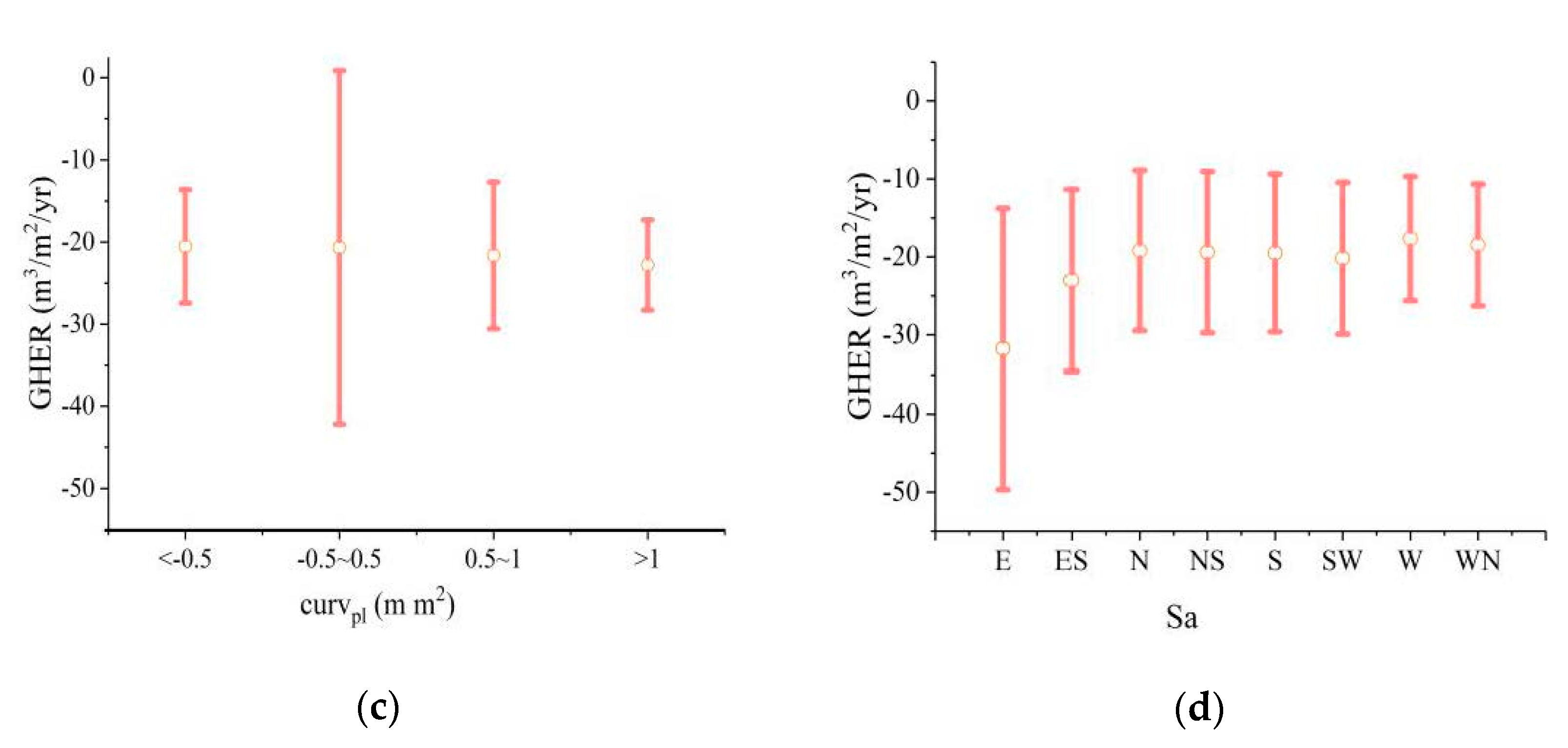
4.3.2. Terrain Attributes
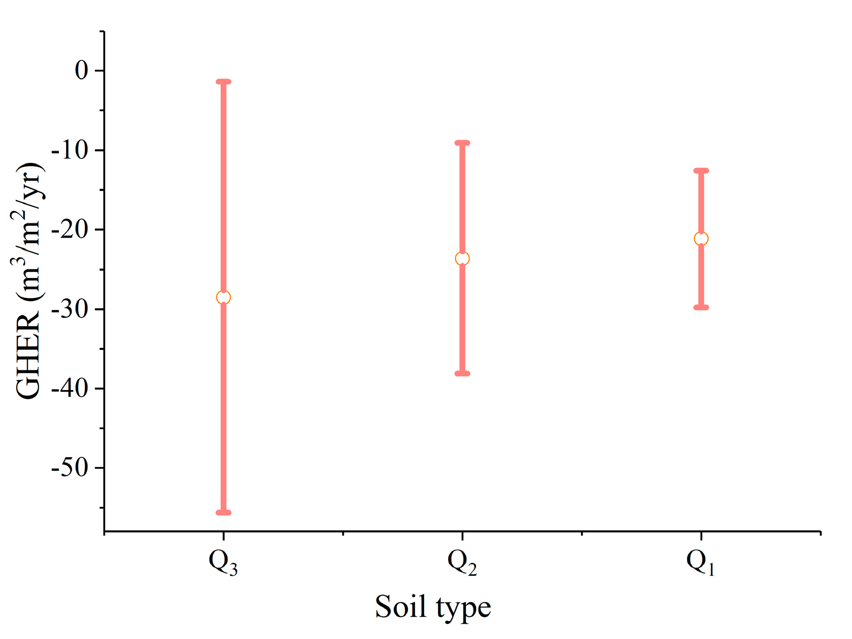
4.3.3. Soil Type
4.4. Estimating the Erosion Rates of the Gully Head
5. Discussion
5.1. Characterization of Gully Head Activities
5.2. Gully Volume Model vs. GHER Model
6. Conclusions
- (i)
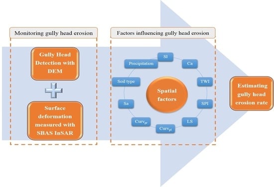
- First, 415 gully heads are extracted by the DEM, and this approach is proven to be feasible by comparing the results with field survey data and digital orthophoto maps. In addition, the ALOS PALSAR data and the SBAS-InSAR method are used to obtain favorable results in monitoring the surface deformation of gully heads, and the SBAS-InSAR results suggest that most of the gully bottoms and flat terrain areas are more stable than the gully heads.
- (ii)
- A simple regression analysis estimates the relation among the erosion rates of gully head erosion, terrain attributes, and soil type. Gully head erosion is strongly positively related to the topographical factors of the slope angle, catchment area, topographic wetness index, and slope length. In contrast, the soil type does not significantly affect the gully head erosion.
- (iii)
- A new framework based on spatial factors (, R2 = 0.889) is proposed to model the gully head erosion. One of the main advantages of combining the erosion rate of the gully head with terrain factors is to simplify the evaluation of the gully head erosion over large areas and long periods, particularly when only environmental information obtained from remote sensing data is available.
- (iv)
- Gully head protection should focus on controlling the terrain attributes of the slope angle and catchment area (e.g., reducing the catchment area of a gully head is an effective method to decrease the gully head erosion). The results of this study can be used for the control and risk assessment of the gully head erosion.
Author Contributions
Funding
Institutional Review Board Statement
Informed Consent Statement
Data Availability Statement
Conflicts of Interest
References
- Belayneh, M.; Yirgu, T.; Tsegaye, D. Current extent, temporal trends, and rates of gully erosion in the Gumara watershed, Northwestern Ethiopia. Glob. Ecol. Conserv. 2020, 24, e01255. [Google Scholar] [CrossRef]
- Su, Z.; Xiong, D.; Dong, Y.; Li, J.; Yang, D.; Zhang, J.; He, G. Simulated headward erosion of bank gullies in the Dry-hot Valley Region of southwest China. Geomorphology 2014, 204, 532–541. [Google Scholar] [CrossRef]
- Xu, Q.; Kou, P.; Wang, C.; Yunus, A.P.; Xu, J.; Peng, S.; He, C. Evaluation of gully head retreat and fill rates based on high-resolution satellite images in the loess region of China. Environ. Earth Sci. 2019, 78, 465. [Google Scholar] [CrossRef]
- Zabihi, M.; Mirchooli, F.; Motevalli, A.; Khaledi Darvishan, A.; Pourghasemi, H.R.; Zakeri, M.A.; Sadighi, F. Spatial modelling of gully erosion in Mazandaran Province, northern Iran. Catena 2018, 161, 1–13. [Google Scholar] [CrossRef]
- Liu, H.; Qian, F.; Ding, W.; Gómez, J.A. Using 3D scanner to study gully evolution and its hydrological analysis in the deep weathering of southern China. Catena 2019, 183, 104218. [Google Scholar] [CrossRef]
- Shi, Q.; Wang, W.; Zhu, B.; Guo, M. Experimental study of hydraulic characteristics on headcut erosion and erosional response in the tableland and gully regions of China. Soil Sci. Soc. Am. J. 2020, 84, 700–716. [Google Scholar] [CrossRef] [Green Version]
- Guo, M.; Wang, W.; Shi, Q.; Chen, T.; Kang, H.; Li, J. An experimental study on the effects of grass root density on gully headcut erosion in the gully region of China’s Loess Plateau. Land Degrad. Dev. 2019, 30, 2107–2125. [Google Scholar] [CrossRef]
- Vanmaercke, M.; Poesen, J.; Van Mele, B.; Demuzere, M.; Bruynseels, A.; Golosov, V.; Bezerra, J.F.R.; Bolysov, S.; Dvinskih, A.; Frankl, A.; et al. How fast do gully headcuts retreat? Earth Sci. Rev. 2016, 154, 336–355. [Google Scholar] [CrossRef]
- Moriasi, D.N.; Arnold, J.G.; Van Liew, M.W.; Bingner, R.L.; Harmel, R.D.; Veith, T.L. Model evaluation guidelines for systematic quantification of accuracy in watershed simulations. Trans. Asabe 2007, 50, 885–900. [Google Scholar] [CrossRef]
- Zhu, H.; Tang, G.; Qian, K.; Liu, H. Extraction and analysis of gully head of Loess Plateau in China based on digital elevation model. Chin. Geogr. Sci. 2014, 24, 328–338. [Google Scholar] [CrossRef] [Green Version]
- Bernatek-Jakiel, A.; Poesen, J. Subsurface erosion by soil piping: Significance and research needs. Earth Sci. Rev. 2018, 185, 1107–1128. [Google Scholar] [CrossRef]
- Oostwoud Wijdenes, D.J.; Bryan, R. Gully-head erosion processes on a semi-arid valley floor in Kenya: A case study into temporal variation and sediment budgeting. Earth Surf. Process. Landf. 2001, 26, 911–933. [Google Scholar] [CrossRef]
- Yang, B.; Yin, K.; Lacasse, S.; Liu, Z. Time series analysis and long short-term memory neural network to predict landslide displacement. Landslides 2019, 16, 677–694. [Google Scholar] [CrossRef]
- Shruthi, R.B.V.; Kerle, N.; Jetten, V.; Abdellah, L.; Machmach, I. Quantifying temporal changes in gully erosion areas with object oriented analysis. Catena 2015, 128, 262–277. [Google Scholar] [CrossRef]
- Addisie, M.B.; Ayele, G.K.; Gessess, A.A.; Tilahun, S.A.; Zegeye, A.D.; Moges, M.M.; Schmitter, P.; Langendoen, E.J.; Steenhuis, T.S. Gully Head Retreat in the Sub-Humid Ethiopian Highlands: The Ene-Chilala Catchment. Land Degrad. Dev. 2017, 28, 1579–1588. [Google Scholar] [CrossRef]
- Guan, Y.; Yang, S.; Zhao, C.; Lou, H.; Chen, K.; Zhang, C.; Wu, B. Monitoring long-term gully erosion and topographic thresholds in the marginal zone of the Chinese Loess Plateau. Soil Tillage Res. 2021, 205, 104800. [Google Scholar] [CrossRef]
- Li, Z.; Zhang, Y.; Zhu, Q.; Yang, S.; Li, H.; Ma, H. A gully erosion assessment model for the Chinese Loess Plateau based on changes in gully length and area. Catena 2017, 148, 195–203. [Google Scholar] [CrossRef]
- Zhao, C.; Lu, Z.; Zhang, Q.; de la Fuente, J. Large-area landslide detection and monitoring with ALOS/PALSAR imagery data over Northern California and Southern Oregon, USA. Remote Sens. Environ. 2012, 124, 348–359. [Google Scholar] [CrossRef]
- Kavats, O.; Khramov, D.; Sergieieva, K.; Vasyliev, V. Monitoring Harvesting by Time Series of Sentinel-1 SAR Data. Remote Sens. 2019, 11, 2496. [Google Scholar] [CrossRef] [Green Version]
- Arabameri, A.; Cerda, A.; Rodrigo, C.; Pradhan, B.; Sohrabi, M.; Blaschke, T.; Tien, B. Proposing a Novel Predictive Technique for Gully Erosion Susceptibility Mapping in Arid and Semi-arid Regions (Iran). Remote Sens. 2019, 11, 2577. [Google Scholar] [CrossRef] [Green Version]
- Wu, Q.; Jia, C.; Chen, S.; Li, H. SBAS-InSAR Based Deformation Detection of Urban Land, Created from Mega-Scale Mountain Excavating and Valley Filling in the Loess Plateau: The Case Study of Yan’an City. Remote Sens. 2019, 11, 1673. [Google Scholar] [CrossRef] [Green Version]
- Berardino, P.; Fornaro, G.; Lanari, R.; Sansosti, E. A new algorithm for surface deformation monitoring based on small baseline differential SAR interferograms. IEEE Trans. Geosci. Remote Sens. 2002, 40, 2375–2383. [Google Scholar] [CrossRef] [Green Version]
- Ferretti, A.; Prati, P.; Rocca, F. Nonlinear Subsidence Rate Estimation Using Permanent Scatterers in Differential SAR Interferometry. IEEE Trans. Geosci. Remote Sens. 2000, 38, 2202–2212. [Google Scholar] [CrossRef] [Green Version]
- Ferretti, A.; Prati, C.; Rocca, F. Permanent scatterers in SAR interferometry. IEEE Trans. Geosci. Remote Sens. 2001, 39, 8–20. [Google Scholar] [CrossRef]
- Hao, J.; Wu, T.; Wu, X.; Hu, G.; Zou, D.; Zhu, X.; Zhao, L.; Li, R.; Xie, C.; Ni, J.; et al. Investigation of a Small Landslide in the Qinghai-Tibet Plateau by InSAR and Absolute Deformation Model. Remote Sens. 2019, 11, 2126. [Google Scholar] [CrossRef] [Green Version]
- Zhao, R.; Li, Z.-W.; Feng, G.-C.; Wang, Q.-J.; Hu, J. Monitoring surface deformation over permafrost with an improved SBAS-InSAR algorithm: With emphasis on climatic factors modeling. Remote Sens. Environ. 2016, 184, 276–287. [Google Scholar] [CrossRef]
- Zhao, F.; Meng, X.; Zhang, Y.; Chen, G.; Su, X.; Yue, D. Landslide Susceptibility Mapping of Karakorum Highway Combined with the Application of SBAS-InSAR Technology. Sensors 2019, 19, 2685. [Google Scholar] [CrossRef] [Green Version]
- Nazari Samani, A.; Ahmadi, H.; Jafari, M.; Boggs, G.; Ghoddousi, J.; Malekian, A. Geomorphic threshold conditions for gully erosion in Southwestern Iran (Boushehr-Samal watershed). J. Asian Earth Sci. 2009, 35, 180–189. [Google Scholar] [CrossRef]
- Thompson, J.R. Quantitative effect of watershed variables on rate of gully-head advancement. Trans. Asae 1964, 7, 54–55. [Google Scholar] [CrossRef]
- Zhu, T.X. Gully and tunnel erosion in the hilly Loess Plateau region, China. Geomorphology 2012, 153–154, 144–155. [Google Scholar] [CrossRef]
- Yuan, M.; Zhang, Y.; Zhao, Y.; Deng, J. Effect of rainfall gradient and vegetation restoration on gully initiation under a large-scale extreme rainfall event on the hilly Loess Plateau: A case study from the Wuding River basin, China. Sci. Total Environ. 2020, 739, 140066. [Google Scholar] [CrossRef] [PubMed]
- Li, C.; Qi, J.; Wang, S.; Yang, L.; Yang, W.; Zou, S.; Zhu, G.; Li, W. A Holistic System Approach to Understanding Underground Water Dynamics in the Loess Tableland: A Case Study of the Dongzhi Loess Tableland in Northwest China. Water Resour. Manag. 2014, 28, 2937–2951. [Google Scholar] [CrossRef]
- Wischmeier, W.H.; Smith, D.D. Predicting Rainfall Erosion Losses: A Guide to Conservation Planning; No. 537; Department of Agriculture, Science and Education Administration: Washington, DC, USA, 1978. [Google Scholar]
- Moore, I.D.; Grayson, R.B.; Ladson, A.R. Digital terrain modelling: A review of hydrological, geomorphological, and biological applications. Hydrol. Process. 1991, 5, 3–30. [Google Scholar] [CrossRef]
- Moore, I.D.; Burch, G.J.; Mackenzie, D.H. Topographic effects on the distribution of surface soil water and the location of ephemeral gullies. Trans. Asae 1988, 31, 1098–1107. [Google Scholar] [CrossRef]
- Desmet, P.J.J.; Poesen, J.; Govers, G.; Vandaele, K. Importance of slope gradient and contributing area for optimal prediction of the initiation and trajectory of ephemeral gullies. Catena 1999, 37, 377–392. [Google Scholar] [CrossRef]
- Desmet, P.J.J.; Govers, G. Comparison of routing algorithms for digital elevation models and their implications for predicting ephemeral gullies. Int. J. Geogr. Inf. Sci. 1996, 10, 311–331. [Google Scholar] [CrossRef]
- Zhou, Y.; Tang, G.A.; Yang, X.; Xiao, C.; Zhang, Y.; Luo, M. Positive and negative terrains on northern Shaanxi Loess Plateau. J. Geogr. Sci. 2010, 20, 64–76. [Google Scholar] [CrossRef]
- Lauknes, T.R.; Zebker, H.A.; Larsen, Y. InSAR Deformation Time Series Using an L1-Norm Small-Baseline Approach. IEEE Trans. Geosci. Remote Sens. 2011, 49, 536–546. [Google Scholar] [CrossRef] [Green Version]
- Chaussard, E.; Wdowinski, S.; Cabral-Cano, E.; Amelung, F. Land subsidence in central Mexico detected by ALOS InSAR time-series. Remote Sens. Environ. 2014, 140, 94–106. [Google Scholar] [CrossRef]
- Nagelkerke, N.J. A note on a general definition of the coefficient of determination. Biometrika 1991, 78, 691–692. [Google Scholar] [CrossRef]
- Frankl, A.; Poesen, J.; Haile, M.; Deckers, J.; Nyssen, J. Quantifying long-term changes in gully networks and volumes in dryland environments: The case of Northern Ethiopia. Geomorphology 2013, 201, 254–263. [Google Scholar] [CrossRef] [Green Version]
- Marzolff, I.; Poesen, J. The potential of 3D gully monitoring with GIS using high-resolution aerial photography and a digital photogrammetry system. Geomorphology 2009, 111, 48–60. [Google Scholar] [CrossRef]
- Zhang, Y.; Zhao, Y.; Liu, B.; Wang, Z.; Zhang, S. Rill and gully erosion on unpaved roads under heavy rainfall in agricultural watersheds on China’s Loess Plateau. Agric. Ecosyst. Environ. 2019, 284, 106580. [Google Scholar] [CrossRef]
- Frankl, A.; Poesen, J.; Scholiers, N.; Jacob, M.; Haile, M.; Deckers, J.; Nyssen, J. Factors controlling the morphology and volume (V)-length (L) relations of permanent gullies in the northern Ethiopian Highlands. Earth Surf. Process. Landf. 2013, 38, 1672–1684. [Google Scholar] [CrossRef] [Green Version]
- Frankl, A.; Poesen, J.; Deckers, J.; Haile, M.; Nyssen, J. Gully head retreat rates in the semi-arid highlands of Northern Ethiopia. Geomorphology 2012, 173–174, 185–195. [Google Scholar] [CrossRef] [Green Version]
- Vandekerckhove, L.; Poesen, J.; Wijdenes, D.O.; Gyssels, G. Short-term bank gully retreat rates in Mediterranean environments. Catena 2001, 44, 133–161. [Google Scholar] [CrossRef]
- Tang, H.; Pan, H.; Ran, Q. Impacts of Filled Check Dams with Different Deployment Strategies on the Flood and Sediment Transport Processes in a Loess Plateau Catchment. Water 2020, 12, 1319. [Google Scholar] [CrossRef]
- Capra, A.; Mazzara, L.M.; Scicolone, B. Application of the EGEM model to predict ephemeral gully erosion in Sicily, Italy. Catena 2005, 59, 133–146. [Google Scholar] [CrossRef]
- Bergonse, R.; Reis, E. Controlling factors of the size and location of large gully systems: A regression-based exploration using reconstructed pre-erosion topography. Catena 2016, 147, 621–631. [Google Scholar] [CrossRef]
- Zucca, C.; Canu, A.; Della Peruta, R. Effects of land use and landscape on spatial distribution and morphological features of gullies in an agropastoral area in Sardinia (Italy). Catena 2006, 68, 87–95. [Google Scholar] [CrossRef]
- Nazari Samani, A.; Ahmadi, H.; Mohammadi, A.; Ghoddousi, J.; Salajegheh, A.; Boggs, G.; Pishyar, R. Factors Controlling Gully Advancement and Models Evaluation (Hableh Rood Basin, Iran). Water Resour. Manag. 2009, 24, 1531–1549. [Google Scholar] [CrossRef]


| Image No. | Incident Angle (°) | Acquisition Date | Polarization |
|---|---|---|---|
| 1 | 38.708 | 1 January 2007 | HH |
| 2 | 38.705 | 16 February 2007 | HH |
| 3 | 38.702 | 4 July 2007 | HH |
| 4 | 38.709 | 19 August 2007 | HH |
| 5 | 38.698 | 4 October 2007 | HH |
| 6 | 38.727 | 19 November 2007 | HH |
| 7 | 38.693 | 4 January 2008 | HH |
| 8 | 38.721 | 19 February 2008 | HH |
| 9 | 38.685 | 5 April 2008 | HH |
| 10 | 38.694 | 21 May 2008 | HH |
| 11 | 38.705 | 6 July 2008 | HH |
| 12 | 38.714 | 6 January 2009 | HH |
| 13 | 38.714 | 21 February 2009 | HH |
| 14 | 38.706 | 9 July 2009 | HH |
| 15 | 38.701 | 24 August 2009 | HH |
| 16 | 38.696 | 9 October 2009 | HH |
| 17 | 38.720 | 9 January 2010 | HH |
| 18 | 38.723 | 24 February 2010 | HH |
| 19 | 38.709 | 12 July 2010 | HH |
| 20 | 38.714 | 12 October 2010 | HH |
| 21 | 38.699 | 12 January 2011 | HH |
| 22 | 38.703 | 27 February 2011 | HH |
| GHER | Sl | Ca | TWI | SPI | LS | Curvpl | Curvpr | Sa | |
|---|---|---|---|---|---|---|---|---|---|
| GHER | 1 | ||||||||
| Sl | 0.768 * | 1 | |||||||
| Ca | 0.895 * | −0.670 * | 1 | ||||||
| TWI | 0.096 | 0.273 * | −0.273 * | 1 | |||||
| SPI | −0.071 | 0.029 | 0.035 | −0.002 | 1 | ||||
| LS | 0.901 * | −0.897 * | −0.900 * | −0.030 | 0.030 | 1 | |||
| Curvpl | −0.016 | 0.001 | 0.049 | 0.120 * | −0.030 | 0.020 | 1 | ||
| Curvpr | −0.034 | 0.039 | 0.044 | −0.004 | −0.053 | 0.039 | −0.030 | 1 | |
| Sa | −0.242 * | 0.112 * | 0.233 * | 0.118 * | 0.066 | 0.190 * | 0.001 | −0.088 | 1 |
| Type | Parameter | Accuracy (R2) | ||
|---|---|---|---|---|
| a | b | c | ||
| Sl | −0.256 | 1.324 | 0 | 0.665 |
| Ca | −0.033 | 1.124 | −1.946 | 0.758 |
| TWI | −0.095 | 2.42 | −5.44 | 0.519 |
| LS | −0.857 | 1.053 | 0 | 0.812 |
Publisher’s Note: MDPI stays neutral with regard to jurisdictional claims in published maps and institutional affiliations. |
© 2021 by the authors. Licensee MDPI, Basel, Switzerland. This article is an open access article distributed under the terms and conditions of the Creative Commons Attribution (CC BY) license (http://creativecommons.org/licenses/by/4.0/).
Share and Cite
Jiang, C.; Fan, W.; Yu, N.; Nan, Y. A New Method to Predict Gully Head Erosion in the Loess Plateau of China Based on SBAS-InSAR. Remote Sens. 2021, 13, 421. https://doi.org/10.3390/rs13030421
Jiang C, Fan W, Yu N, Nan Y. A New Method to Predict Gully Head Erosion in the Loess Plateau of China Based on SBAS-InSAR. Remote Sensing. 2021; 13(3):421. https://doi.org/10.3390/rs13030421
Chicago/Turabian StyleJiang, Chengcheng, Wen Fan, Ningyu Yu, and Yalin Nan. 2021. "A New Method to Predict Gully Head Erosion in the Loess Plateau of China Based on SBAS-InSAR" Remote Sensing 13, no. 3: 421. https://doi.org/10.3390/rs13030421
APA StyleJiang, C., Fan, W., Yu, N., & Nan, Y. (2021). A New Method to Predict Gully Head Erosion in the Loess Plateau of China Based on SBAS-InSAR. Remote Sensing, 13(3), 421. https://doi.org/10.3390/rs13030421