Tomographic Performance of Multi-Static Radar Formations: Theory and Simulations

Abstract

3D imaging of Earth’s surface layers (such as canopy, sub-surface, or ice) requires not just the penetration of radar signal into the medium, but also the ability to discriminate multiple scatterers within a slant-range and azimuth resolution cell. The latter requires having multiple radar channels distributed in across-track direction. Here, we describe the theory of multi-static radar tomography with emphasis on resolution, SNR, sidelobes, and nearest ambiguity location vs. platform distribution, observation geometry, and different multi-static modes. Signal-based 1D and 2D simulations are developed and results for various observation geometries, target distributions, acquisition modes, and radar parameters are shown and compared with the theory. Pros and cons of multi-static modes are compared and discussed. Results for various platform formations are shown, revealing that unequal spacing is useful to suppress ambiguities at the cost of increased multiplicative noise. In particular, we demonstrate that the multiple-input multiple-output (MIMO) mode, in combination with nonlinear spacing, outperforms the other modes in terms of ambiguity, sidelobe levels, and noise suppression. These findings are key to guiding the design of tomographic SAR formations for accurate surface topography and vegetation mapping.

1. Introduction

Airborne and space-based radar imaging of Earth’s surface for scientific, civilian, and surveillance purposes has been an active field of research since the 1950s. The Earth’s surface can be imaged from space using a single radar platform employing the synthetic aperture radar (SAR) technique, first demonstrated with the Seasat satellite [1]. By virtue of the SAR measurement process and side-looking geometry, radar signals scattered from targets located at about the same distance from the radar antenna and within the SAR resolution cell are superimposed and indistinguishable in the final two-dimensional SAR image. At least two interferometric SAR (InSAR) acquisitions are needed to recover the third dimension, i.e., the location or the change of the microwave scattering phase center above the Earth’s surface [2,3,4,5]. In order to resolve distinct targets located at different heights and within the same slant-range resolution cell, multiple radar signals transmitted and/or received from different radar look angles are required. The acquisition and processing of these signals that lead to vertical imaging of natural and human-made media is known as SAR tomography, or TomoSAR [6,7,8]. The image consisting of multiple layers along the vertical direction or along the elevation direction—i.e., perpendicular to the look-angle direction—is referred to as SAR tomogram. SAR tomograms can be one-dimensional (1D), two-dimensional (2D), or three-dimensional (3D) depending on whether range and/or azimuth dimensions are displayed. Multiple signals with look-angle diversity can be acquired by the same platform drifting at each pass (repeat-pass TomoSAR), by a multi-static formation of several platforms in which one or more platforms transmit radar pulses and a set of platforms receives the scattered signals (single-pass TomoSAR), or by a combination of the two acquisitions strategies.

Several works on TomoSAR have been published since the first demonstrations and signal data models appeared in the literature [6,7,9,10,11,12,13]. Over the past two decades, SAR tomography has been applied with increasingly promising results to forests [12,13,14,15,16,17,18,19,20,21,22], croplands [23], urban environment [24,25,26,27,28,29], and, more recently, ice [30] and snow [31,32,33,34,35]. All these natural media share a volumetric structure causing multiple scatterers to lie within the same radar resolution cell, which TomoSAR can identify and disentangle, providing opportunities for resolving the internal components of the media. Comparative TomoSAR retrievals of vertical structure have been shown at multiple frequencies, from X band, to L and P bands [36,37]. Tomographic SAR algorithms have been tested from different platforms, including tower-based structures [32,38], airborne [7,39], and even spaceborne where a broad range of baseline diversity is typically difficult to achieve [40]. Algorithms aiming to reconstruct the vertical reflectivity profiles from a set of multi-baseline SAR acquisitions have been developed extensively and are typically grouped into model and non-model based. Model-based algorithms [41] use statistical or physics-based assumptions for the vertical target reflectivity with the aim to improve the quality of the vertical imaging or reduce the system constraints (e.g., the number of baselines). Non-model-based algorithms make no assumptions and leverage the intrinsic imaging capabilities of TomoSAR. Algorithms such as back-projection, Fourier, Capon [42], or the more recent backscatter-height histograms approach [43] belong to this group. While these algorithms are constantly improved and applied to new experimental and simulated data, research in TomoSAR is currently active on two main fronts: (1) how to extract bio-physical parameters from SAR tomograms [43,44,45], and (2) how to optimize the multi-static SAR systems in order to maximize the quality of tomograms with constrained resources [36,46,47,48].

The quality of tomographic SAR images depends not only on the single radar instrument performance (e.g., signal-to-noise ratio and range sidelobes), but also on the distribution of the platforms as well as the relative orientation between platform baselines and look direction [49]. In general, the spacing among the platforms determines the locations of the ambiguities (i.e., target replicas) within the tomogram, and the length of the overall baseline perpendicular to the look direction determines the tomogram resolution. The sidelobes for each point target also depends on the platform distribution in addition to the windowing applied, if any [36,50]. On the other hand, the actual (instead of perpendicular to look angle) spacing and baseline required to meet given values of resolution and ambiguity location depend on the baseline tilt. Finally, the degree to which these considerations apply to tomographic imaging depends on the choice of the transmit/receive platform configuration, in this paper referred to as multi-static or tomographic mode. In a distributed formation of radar satellites, multiple signals can be acquired in three main modes: (1) SAR (or ping-pong), where each platform transmits/receives sequentially as in actual along-track SAR; (2) single-input multiple-output (SIMO), where a single platform transmits and all platforms receive; and (3) multiple-input multiple-output (MIMO), where multiple platforms transmit sequentially and multiple platforms receive simultaneously for each transmit platform. Although the MIMO mode can operate with any subset of receive and transmit platforms, here we consider the case of full MIMO, i.e., when all platforms in the formation operate as both transmitters and receivers.

In this article, we provide a comparative assessment of TomoSAR performance as a function of key observation and instrument parameters that can be used towards the design of a multi-static tomographic formation [51,52]. The equations governing the dependence of the tomographic image quality (e.g., resolution and the nearest ambiguity location) on platform geometry (e.g., platform distribution, orientation, look angle, and altitude) and radar parameters (e.g., frequency and windowing) are presented and discussed for three different multi-static modes (SAR, SIMO, and MIMO) in Section 2. The minimum number of platforms required for a specific resolution and ambiguity location for each mode is also provided. Then, our simulation approach is described in Section 3 with the aim to provide radar scientists and engineers with a simple yet effective tool to explore the parameter space when designing airborne or spaceborne tomographic radar missions. Simulated 1D and 2D tomograms for various target and platform distributions are shown and discussed in Section 4 to highlight how tomogram quality changes with platform baseline orientation and look angle, as well as radar parameters (specifically frequency, bandwidth, SNR, PRI, and windowing). Different multi-static modes (SAR, SIMO, and MIMO) are analyzed and simulation results are in agreement with theory. Furthermore, the performance of each mode in terms of robustness to random noise is demonstrated.

The pros and cons of each multi-static mode, in terms of hardware and design complexity and tomographic performance (resolution, ambiguity, sidelobes, and SNR), are discussed in Section 5. Among the various findings, results show that for a given platform distribution, the SAR mode offers the best resolution and SIMO mode has the worst resolution, whereas MIMO resolution performance lies in between the two. On the contrary, SAR mode has the worst ambiguity location, whereas SIMO and MIMO modes exhibit the same performance. MIMO has significantly higher SNR and lower sidelobes than SAR and SIMO. Results for various platform distributions are also shown revealing that unequal spacing is useful to suppress ambiguities at the cost of increased multiplicative noise (processing sidelobes).

In particular, we demonstrate that the MIMO mode, in combination with nonlinear spacing, outperforms the other modes in terms of ambiguity, sidelobes levels, and noise suppression. Conclusions are drawn in Section 6 with an outlook to future directions of this work.

2. Theory of Tomographic Imaging

The simplified geometry of tomographic imaging is shown in Figure 1 along with the parameters that characterize the geometry of the platform distribution and imaged scene. In this section, we use Figure 1 as a reference to develop the underlying theory and, in Section 3, to describe our simulation approach. Some of equations presented hereafter appeared in similar or simplified forms in previous papers (see in [8] and references therein cited), and are revisited and extended here to provide context for this study.

The platforms are assumed to be distributed along a line in the across-track plane and can transmit and receive or be receive-only depending on the tomographic mode (SAR, SIMO, or MIMO). Platforms can be spaced equally or unequally. For equally distributed platforms, analytical formulas for spatial resolution and nearest ambiguity location exist and are presented in this section. For unequally spaced platforms, only simulation results are available and are presented in Section 4.3. For analytical solutions, platform positions are projected onto the axis perpendicular to look direction ($\underset{\_}{n}$) using the baseline tilt angle ($\alpha$) and look angle ($\theta$). Perpendicular spacing and baseline length is then used to calculate the nearest ambiguity location and spatial resolution along $\underset{\_}{n}$. The quality of 2D tomographic images on the ground-range (vertical and horizontal) plane depends on the tomographic performance along look direction ($\underset{\_}{r}$) and along $\underset{\_}{n}$, which are coupled via look angle and local terrain slope ($\underset{\_}{\epsilon }$). Therefore, in addition to resolution and ambiguity along $\underset{\_}{n}$ (elevation or perpendicular to look direction), we also include range resolution and ambiguity along $\underset{\_}{r}$ (slant range or look direction).

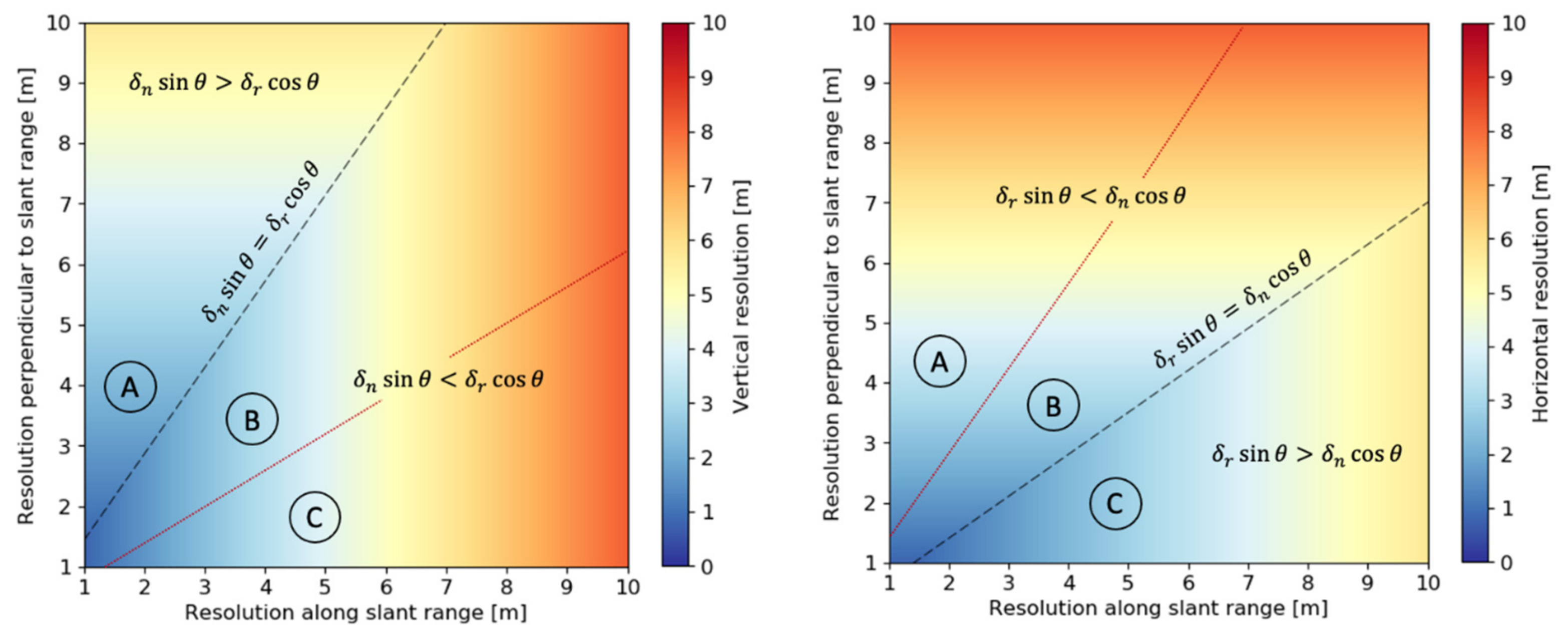
2.1. Resolution

Two scatterers in the scene imaged by a radar can be resolved if their slant-range distances differ at least by 1–2 times the range resolution (${\delta }_r$), depending on the tomographic mode,

$${\delta }_r=w_r\frac{c}{2B}$$

(1)

where $c$ is the speed of light, $B$ is the transmitted signal bandwidth, and $w_r$ is the expansion coefficient that accounts for the effects of windowing, typically applied to reduce sibelobes. When no windowing is applied, then $w_r=1$; otherwise, $w_r>1$. Note that, without windowing, the resolution given by (1) corresponds to the Rayleigh (peak-to-null) resolution, which is equivalent to the ~4 dB resolution (not 3 dB, as usually assumed) [50] (Section 20.7.4).

The scatterers within the same slant range resolution cell can be resolved using the tomography technique. The tomographic resolution along $\underset{\_}{n}$ (${\delta }_n$) depends on the maximum baseline length. Its equation is similar to the SAR resolution equation, with synthetic aperture length replaced by the tomographic baseline length [8],

$${\delta }_n=w_n\frac{\lambda r_0}{p_{\delta }{L}_n}$$

(2)

where $\lambda$ is center wavelength, $r_0$ is slant range at the center of the aperture, $p_{\delta }$ is the multi-static mode resolution coefficient shown below in (7), $L_n$ is the maximum perpendicular baseline length, and $w_r$ is the expansion coefficient due to windowing typically applied to reduce sibelobes.

By focusing the complex phase vector of each platform to the point target location and summing over platforms, the point spread function (PSF) of tomographic processing (without windowing and in relative power units) is derived for the SAR mode and equal spacing as

$${\left|I\left(n\right)\right|}^2={\left|\frac{sin\left(\frac{2\pi }{\lambda r_0}N{\mu }_{n}n \right)}{sin\left(\frac{2\pi }{\lambda r_0}{\mu }_{n}n \right)}\right|}^2$$

(3)

where ${\mu }_n$ is perpendicular platform spacing, $N$ is the number of platforms, and $n$ is the distance from the point target position in the perpendicular to look angle direction ($\underset{\_}{n}$). As the sinusoidal radar signal represents voltage (or current), power of the signal is proportional to the square of the signal. This is also the case for signal processing outputs such as the PSF.

The tomographic Rayleigh (peak-to-null) resolution for the SAR mode can be found by equating (3) to zero and solving for $n$. In fact, without windowing ($w_n=1$), the resolution given by (2) corresponds exactly to the one-sided Rayleigh (peak-to-null) resolution when the maximum perpendicular baseline $L_n$ is taken as $L_n=N{\mu }_n$, which corresponds to the maximum distance between platforms, i.e.,$\left(N-1\right){\mu }_n$, plus one platform spacing (${\mu }_n$) projected onto $\underset{\_}{n}$ as shown in Figure 1.

Spatial resolution is usually defined as the two-sided distance at which the signal power level of the PSF is at a specific level (usually in dB scale) relative to the peak of the PSF. For example, the 3 dB resolution is equal to twice the distance at which the power level of the PSF reduces to half of the peak. The tomographic PSR power level (relative to the peak of the PSR) corresponding to the resolution given by (2) can be found by evaluating (3) at $n={\delta }_n/2$, the result of which is shown in Figure 2. Figure 2 shows the variation of the power level relative to the peak with respect to the number of platforms when baseline is taken as the maximum distance among platforms ($L_n= \left(N-1\right){\mu }_n$) and when baseline is taken as the number of platforms multiplied by spacing ($L_n=N{\mu }_n$). It can be observed that the resolution calculated by (2) corresponds to ~4 dB two-sided resolution when number of platforms ($N$) is large. For smaller $N$, this is no longer valid. It can be seen that $L_n=N{\mu }_n$ is a better choice for resolution as its power level variation for small number of platforms is much less than the $L_n= \left(N-1\right){\mu }_n$ option and is always between 3 dB and 4 dB. Therefore, for resolution purposes, we recommend using $L_n=N{\mu }_n$, which is one spacing larger than the maximum distance among platforms as shown in Figure 1.

The form and derivation of (2) is similar to that of the resolution of a synthetic aperture radar (SAR) or the beamwidth of a phased array antenna. The main difference with a single platform SAR is that having multiple platforms allows for different multi-static modes. The main difference with phased-array antenna is that the platforms do not all have to transmit at the same time which negates the need to electronically scan the beam on transmit.

The perpendicular baseline ($L_n$) depends on the actual baseline length ($L$), the baseline tilt angle ($\alpha$), and the look angle ($\theta$) [2],

$$L_n=L cos\left(\left|\theta -\alpha \right|\right)$$

(4)

which is valid for $r_0\gg L$ (to keep $\theta$ approximately constant along the aperture).

For flat surfaces, the slant range can be written as

$$r_0=H/cos\theta$$

(5)

where $H$ is the (average) platform altitude. This is valid when $H\ll r_p$ (where $r_p$ is planetary radius) and $\theta$ is sufficiently small. Otherwise, the law of cosines needs to be used to calculate $r_0$ accurately. For our purposes, here we assume flat surface for simplicity, which does not change the main conclusions of this paper.

Combining (2), (4), and (5), the tomographic resolution equation as a function of SAR instrument and formation parameters becomes

$${\delta }_n=\frac{w_n}{p_{\delta }}\frac{\lambda H}{L}\frac{1}{cos\left(\left|\theta -\alpha \right|\right)cos\theta }$$

(6)

The resolution coefficient ($p_{\delta }$) depends on the multi-static mode [46] and, for MIMO, whether two-sided 3.9 dB resolution or one-sided peak-to-null (Rayleigh) resolution is considered:

$$\begin{gathered} p_{\delta }=2 \mathrm{for} \mathrm{SAR} \mathrm{mode} \\ {p}_{\delta }=1 \mathrm{for} \mathrm{SIMO} \mathrm{mode} \\ {p}_{\delta } \cong 1.38 \mathrm{for} \mathrm{MIMO} \mathrm{mode} (3.9 \mathrm{dB} \mathrm{two}\text{-}\mathrm{sided} \mathrm{resolution}) \\ {p}_{\delta }=1 \mathrm{for} \mathrm{MIMO} \mathrm{mode} (\mathrm{peak}\text{-}\mathrm{to}\text{-}\mathrm{null} \mathrm{Rayleigh} \mathrm{resolution}) \end{gathered}$$

(7)

where SAR, SIMO, and MIMO are the multi-static modes introduced in Section 1. The $p_{\delta }$ values for SIMO and MIMO are derived empirically from simulation results. In the SIMO mode (similar to phased array antenna), the range (and therefore phase) difference is only one-way, resulting in a resolution twice that of the SAR mode, in which the range difference is two-way (similar to along-track SAR). MIMO mode is a combination of one-way and two-way range differences and therefore has a resolution in between the SAR and SIMO modes.

In the applications of SAR tomography, it is informative to consider the resolution of the final tomogram in ground range coordinates. Care must be taken when projecting the resolutions ${\delta }_r$ and ${\delta }_n$ onto the vertical ($\underset{\_}{z}$) and horizontal ($\underset{\_}{x}$) axes. In particular, because the shape of the tomographic resolution cell is intrinsically different than the shape of the single-platform SAR resolution cell, the horizontal resolution of a tomogram does not equal the traditional SAR range resolution projected onto $\underset{\_}{x}$, i.e., ${\delta }_r/sin\left(\theta \right)$. Figure 3 illustrates how the relative sizes of the resolution cell along the range and elevation directions determine the vertical and horizontal resolutions. The vertical extent of the tomographic resolution cell (gray shape in Figure 3) is either the projection of ${\delta }_n$ or ${\delta }_r$ onto the $\underset{\_}{z}$ axis, whichever is larger. Similarly, the horizontal extent of the tomographic resolution cell is either the projection of ${\delta }_n$ or ${\delta }_r$ onto the $\underset{\_}{x}$ axis, whichever is larger. Therefore, the vertical and horizontal resolutions, indicated, respectively, by ${\delta }_z$ and ${\delta }_x$, can be written as

$$\begin{gathered} {\delta }_z=\max ({\delta }_{nz}, {\delta }_{rz})= \max \left({\delta }_{n}sin\theta , {\delta }_{r}cos\theta \right) \\ {\delta }_x=\max ({\delta }_{nx}, {\delta }_{rx})= \max \left({\delta }_{n}cos\theta , {\delta }_{r}sin\theta \right) \end{gathered}$$

(8)

where ${\delta }_{nz}$ and ${\delta }_{nx}$ are the vertical and horizontal projections of ${\delta }_n$, respectively, and ${\delta }_{rx}$ and ${\delta }_{rz}$ are the vertical and horizontal projections of ${\delta }_r$, respectively (cf. Figure 3). This result implies that the vertical resolution of a tomogram may depend on the range bandwidth, and the horizontal resolution may be driven by the tomographic baseline, contrary to the common belief. More importantly, according to (8), both the vertical and horizontal resolutions may depend on ${\delta }_n$, and therefore on $p_{\delta }$, which means that the selection of the tomographic mode (SAR, SIMO, or MIMO) provides some control on both vertical and horizontal tomogram resolutions. Note that vertical and horizontal tomographic resolutions can be defined alternatively by taking the inner width and length of the resolution cell (i.e., the distances between the centers of adjacent resolution cells along $\underset{\_}{z}$ and $\underset{\_}{x}$). For the purposes of this study, we limit the discussion to the resolution convention illustrated in Figure 3. To understand the implications of (8), Figure 4 shows how ${\delta }_z$ and ${\delta }_x$ change as a function of ${\delta }_n$ and ${\delta }_r$ for $\theta =35°.$ Consider a vertical transect in Figure 4 (i.e., constant slant range resolution ${\delta }_r$). For small values of ${\delta }_n$, the vertical and horizontal resolutions do not change regardless of the value of ${\delta }_n$ and up to a threshold value that depends on the look angle (dashed tilted line). Beyond the dashed line, for large values of ${\delta }_n$, the vertical and horizontal resolutions increase with ${\delta }_n$. Note that the threshold values (tilt of the dashed line) are different between vertical and horizontal resolutions. The dotted red line is used in one plot to illustrate the position of the dashed line in the other plot. Consequently, we can identify three regions in the plots of Figure 1: Region-A, where ${\delta }_n$ determines the values of both ${\delta }_z$ and ${\delta }_x$; Region-B, where the values of ${\delta }_z$ and ${\delta }_x$ depend on either ${\delta }_n$ or ${\delta }_r$; and Region-C, where ${\delta }_r$ determines the values of both ${\delta }_z$ and ${\delta }_x$. As the look angle approaches 45°, Region-B narrows until the dashed line and the dotted line overlap.

2.2. Ambiguities

Ambiguous returns, also referred to as target replicas, occur when platform spacing is periodic [7,8]. They occur along $\underset{\_}{n}$ with spacing inversely proportional to platform spacing. The location of the nearest (relative to actual target) ambiguity is important because it contributes to determine the maximum extent of the target that can be imaged without overlapping replicas. Note that even when the scene of interest is smaller than the nearest ambiguity location, ambiguous replicas of targets outside the scene of interest can still fall into the scene of interest. Therefore, it is desired that the nearest ambiguity is outside the maximum extent of all targets (not just the scene of interest) along $\underset{\_}{n}$, which depends not only on target heights but also on the look angle and local terrain slope. Importantly, a narrow antenna beam along $\underset{\_}{n}$ can suppress ambiguities, but here we assume that the antenna beam is wide such that its ambiguity suppression effect is neglected.

Based on Figure 1, the ambiguities (replicas) along $\underset{\_}{n}$ relative to target ($A_n^k$) occur at [8]

$$A_n^k=k\frac{\lambda r_0}{p_a{\mu }_n}$$

(9)

where $k$ is an integer other than 0 (±1, ±2, etc.), ${\mu }_n$ is platform spacing projected along $\underset{\_}{n}$, and $p_a$ is the ambiguity location coefficient that changes depending on the multi-static mode.

The parameter ${\mu }_n$ depends on the platform spacing ($\mu$), the baseline tilt angle ($\alpha$), and the look angle ($\theta$):

$${\mu }_n=\mu cos\left(\left|\theta -\alpha \right|\right)$$

(10)

which is valid for $r_0\gg L$ (to keep $\theta$ approximately constant along the aperture). Combining (5), (9), and (10), and taking $k=\pm 1$, the nearest ambiguity for a flat surface occurs at

$$A_n^1= \pm \frac{\lambda r_0}{p_a{\mu }_n}= \pm \frac{\lambda H}{p_a\mu cos\left(\left|\theta -\alpha \right|\right) cos \theta }$$

(11)

where the ambiguity location coefficient ($p_a$) is

$$\begin{gathered} p_a=2 \mathrm{for} \mathrm{SAR} \mathrm{mode} \\ {p}_a=1 \mathrm{for} \mathrm{SIMO} \mathrm{mode} \\ {p}_a=1 \mathrm{for} \mathrm{MIMO} \mathrm{mode} \end{gathered}$$

(12)

The value of $p_a$ for the SAR mode can be derived from (3) by finding the periodicity of the PSF. The values of $p_a$ for the SIMO and MIMO modes are derived empirically from simulation results which are presented in Section 4. Similar to the resolution ${\delta }_n$ in (6), the nearest ambiguity occurs at half the distance for SAR mode as compared to the SIMO and MIMO modes due to the two-way phase differences unique to the SAR mode. However, unlike resolution, the ambiguity location for MIMO and SIMO are the same (however, the sidelobes for MIMO are significantly less than SIMO and SAR as will be demonstrated in Section 4). Making platform spacing nonuniform (unequal) can significantly weaken the ambiguity replicas at the cost of increased sidelobes, as will be demonstrated in Section 4.

The scene extent is usually defined in the vertical ($\underset{\_}{z}$) and horizontal ($\underset{\_}{x}$) planes. In many applications of TomoSAR, the distributed target extent along $\underset{\_}{x}$ is much larger than the target extent along $\underset{\_}{z}$ (i.e., tree heights). Therefore, the maximum scene extent along $\underset{\_}{x}$ is usually limited by either the antenna beamwidth or pulse-limited length, whichever is smaller. However, the maximum scene extent along $\underset{\_}{z}$ is usually limited by the target heights (which is usually much smaller than beamwidth and pulse limited lengths).

Based on Figure 1, the required minimum distance for nearest ambiguity along $\underset{\_}{n}$ ($A_n^{req}$) can be defined in terms of the maximum height ($h_z^{max}$) of the targets (e.g., vegetation) by taking into consideration the look angle and local terrain slope ($\epsilon$)

$$A_n^{req}=h_n^{max}=h_z^{max}\frac{cos\epsilon }{sin\left(\theta -\epsilon \right)}$$

(13)

The ratio of $h_n^{max}/h_z^{max}$ is shown in Figure 5:

Figure 5 and (13) reveal that required ambiguity location ($A_n^{req}$) is larger for smaller look angle (if slope is constant), larger for larger slope (if look angle is constant), and can be very large if the difference between look angle and local slope is small. In the latter case, $A_n^{req}$ would be defined either by the antenna across-track beamwidth or by the extent of the sloped surface, whichever is smaller. In the nadir looking and no slope case ($\theta =\epsilon =0^{\circ }$), horizontal resolution would be defined by tomographic resolution, vertical resolution would be defined by the range resolution, and the antenna across-track beamwidth would be critical to suppress the ambiguities as the tomographic ambiguity location requirement would no longer be based on tree heights.

Range ambiguities, i.e., ambiguities along $\underset{\_}{r}$ relative to target ($A_r^k$), occur at

$$A_r^k=k\frac{c}{2f_p}$$

(14)

where $k$ is an integer other than 0 (±1, ±2, etc.), $c$ is speed of light, and $f_p$ is the pulse repetition frequency (PRF).

Interestingly, even though range ambiguities usually occur at relatively long distances compared to the scene of interest, there can be targets at long horizontal distances whose replicas fall onto the scene of interest (especially the multiple replicas along both $\underset{\_}{r}$ and $\underset{\_}{n}$). This is illustrated in Figure 6, where it is shown how multiple replicas can determine the maximum unambiguous scene extent. Figure 6 also shows how making the antenna beam narrower is an effective way to avoid ambiguities in the scene of interest, or alternatively, to extend the scene of interest without introducing ambiguities.

2.3. Minimum Number of Platforms

The tomographic baseline ($L$) and the platform spacing ($\mu$) control the tomographic resolution (${\delta }_n$) and nearest ambiguity location ($A_n^1$), respectively. Combining (6) and (11), it is possible to define the minimum number of platforms ($N$) required to meet given requirements for tomographic resolution and nearest ambiguity location:

$$N\ge \frac{L}{\mu }=\frac{L_n}{{\mu }_n}=\frac{w_n\lambda r_0/p_{\delta }{\delta }_n^{req}}{\lambda r_0/p_a{A}_n^{req}}=w_{n}p\frac{h_n^{max}}{{\delta }_n^{req}}=w_{n}p\frac{h_z^{max}}{{\delta }_n^{req}}\frac{cos\epsilon }{sin\left(\theta -\epsilon \right)}$$

(15)

where $p=p_a/p_{\delta }$ is 1 for SAR and SIMO and ~0.7 for MIMO. Equal platform spacing is assumed. As expected, the required minimum number of platforms is larger for taller targets and finer tomographic resolution. The MIMO mode requires approximately two-thirds of the platforms required in SAR and SIMO modes to achieve the same resolution and ambiguity performance. The required number of platforms and its dependence on various parameters are further discussed in Section 4.1.

3. Tomography Simulations

In this section, we describe our tomographic simulation approach for assessing and comparing tomographic performance. We adopt two strategies for simulation. In the first strategy, platforms and targets are distributed in one dimension (1D) along the $\underset{\_}{n}$ axis, assuming that all target returns are in the same range resolution cell. In the second strategy, platforms and targets are distributed in two dimensions (2D) on the horizontal and vertical plane. While, in general, simulations in 1D can be considered as a particular case of simulations in 2D, here we show how even simplified 1D simulations scenarios can be an effective tool to study key characteristics of tomograms. In particular, simulations in 1D are used in Section 4 to reveal how the tomographic point spread function (PSF) for the three multi-static modes changes as a function of observation and radar parameters. In order to analyze metrics such as resolution, ambiguity, and sidelobes, 1D simulations may be sufficient, whereas to highlight the imaging characteristics of tomography, 2D simulations are required. Hereafter, we provide detailed equations to guide the implementation of both 1D and 2D tomographic simulations.

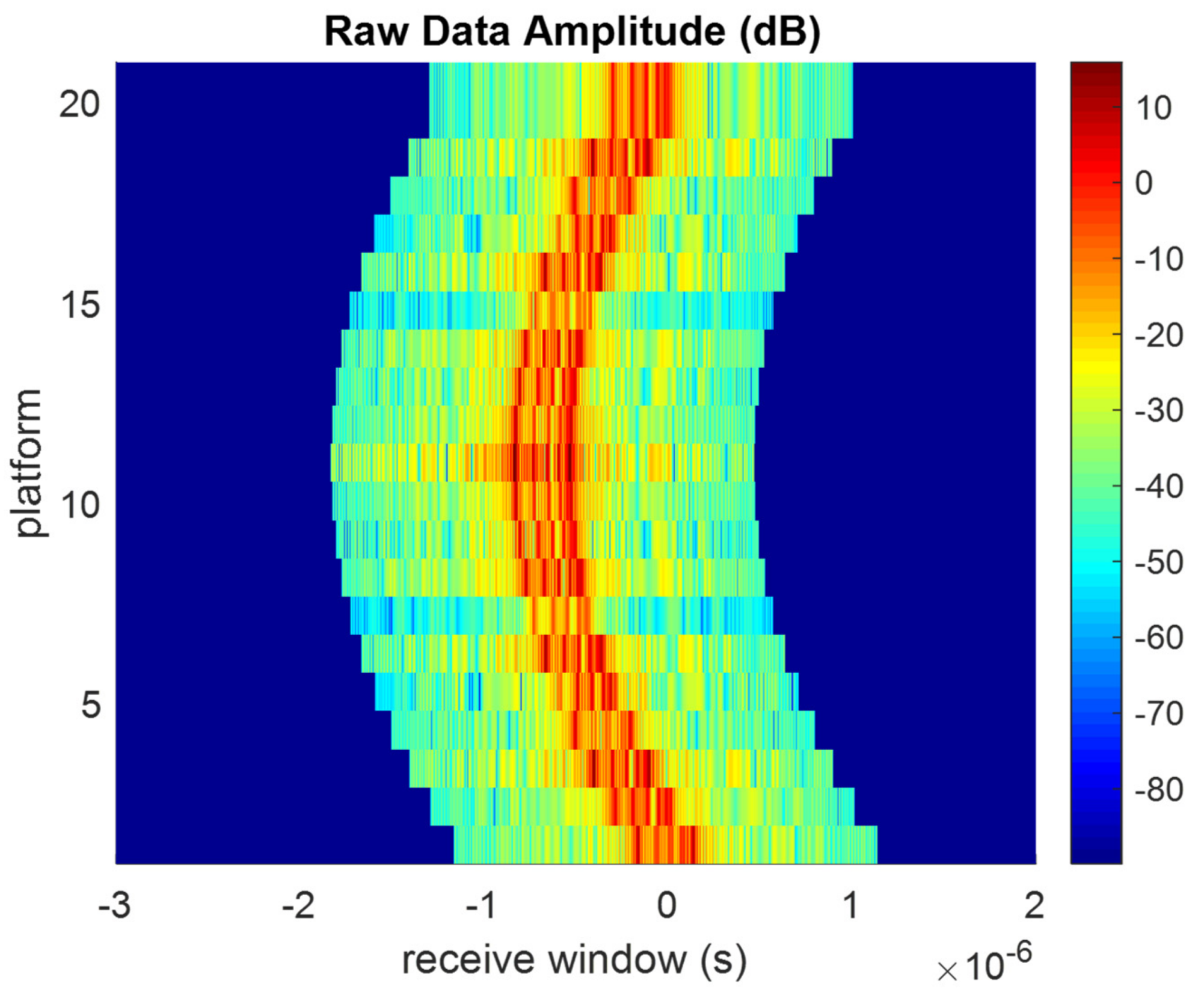
3.1. Raw Data Generation in 1D

Raw tomographic data are simulated by summing the vectors of complex signals received from all scatterers at each platform position. Assuming the platforms are identical, the relative amplitude of each complex signal vector depends mainly on the relative range and radar cross section (RCS) of each target. If the antenna beam is narrow and the tomographic aperture is large, the amplitude can also vary due to variation of antenna gain along elevation. Here, we assume that the antenna beamwidth is sufficiently large and thus its effects are negligible. We do allow for RCS variations from target to target, but it is assumed that the RCS of each target is uniform across the narrow range of look angles spanning the tomographic aperture. Note that this last assumption would not be valid for large bistatic angle systems. The phase of each signal vector is sensitive (especially for higher frequencies) to the slant range variation from target to target and platform to platform, therefore enabling fine resolution (relative to pulse or beam limited resolution) along $\underset{\_}{n}$.

The observation geometry used to generate raw data is illustrated in Figure 7. For the purposes of 1D simulations, it is sufficient to assume that both platforms and targets (input scene) are distributed along elevation ($\underset{\_}{n}$).

The equations governing the tomographic raw data generation for the three modes are

$$\begin{gathered} \mathrm{SAR}: R\left(m\right)={{\displaystyle \sum }}_{k=1}^K{a}_k{e}^{-j\frac{4\pi }{\lambda }{r}_{mk}}+{\tau }_m\hspace{1em}\mathrm{with} m= m_{tx}=m_{rx}\in \left\{1, 2,\dots ,M\right\} \\ \mathrm{SIMO}: R\left(m_{rx}\right)={{\displaystyle \sum }}_{k=1}^K{a}_k{e}^{-j\frac{2\pi }{\lambda }\left(r_{1k}+r_{m_{rx}k}\right)}+{\tau }_m\hspace{1em}\mathrm{with} m_{tx}=1 \mathrm{and} m_{rx}\in \left\{1, 2,\dots ,M\right\} \\ \mathrm{MIMO}: R\left(m_{tx},m_{rx}\right)={{\displaystyle \sum }}_{k=1}^K{a}_k{e}^{-j\frac{2\pi }{\lambda }\left(r_{m_{tx}k}+r_{m_{rx}k}\right)}+{\tau }_m \mathrm{with} m_{tx}, m_{rx}\in \left\{1, 2,\dots ,M\right\} \end{gathered}$$

(16)

where $R\left(\cdot \right)$ is the complex raw data for the mth transmit ($m_{tx}$) or receive ($m_{rx}$) platform, $m$ is the transmit/receive platform for SAR, M is total number of platforms, K is the total number of point targets, $a_k$ is the reflectivity or RCS of each target, $\lambda$ is the central wavelength, $r_{mk}$ is the slant range between the mth platform and kth target, $r_{1k}$ is the slant range for SIMO mode between the fixed TX platform and kth target, and ${\tau }_m$ is the random noise (mostly thermal) which is different for each TX/RX platform pair but independent of targets.

This forward projection transforms the target (or input scene) space of size K (location and reflectivity per each target) to the complex data space of size 1 × M (for SAR and SIMO) or M × M (for MIMO). The generated raw data consist of a complex value (amplitude and phase) per TX/RX pair. Note that, as MIMO mode coherently combines M² independent samples (vs. M for SAR and SIMO), the robustness of MIMO to random noise is significantly better than SAR and SIMO, especially if M is large.

3.2. Tomogram Generation in 1D

A tomographic image is generated using the inverse process of raw data generation as illustrated in Figure 8. First, an output grid of regularly spaced samples (pixels) is defined. Then, each sample is focused by compensating the relative phase of each raw data vector for that point (regardless of whether a target exists at that point). Finally, the phase-compensated complex vector for each platform pair is coherently summed, and its amplitude is taken to obtain the intensity at that point. If there is actually a point target at that location, the focused pixel is going to be relatively bright (depending on target reflectivity). This focusing technique is also known as time-domain back-projection (TDBP) and can be considered as the ideal matched filter for tomography [18,53]. Furthermore, unlike FFT-based algorithms, TDBP allows for arbitrary distribution of platforms, targets, and image pixels. The main disadvantage of TDBP is that processing time is slower relative to the FFT-based methods.

The equations used to generate the 1D tomograms are

$$\begin{gathered} \mathrm{SAR}: I\left(s^p\right) = \left|{{\displaystyle \sum }}_{m=1}^{M}R\left(m\right) e^{j\frac{4\pi }{\lambda }{r}_{mp}}\right| \\ \mathrm{SIMO}: I\left(s^p\right) = \left|{{\displaystyle \sum }}_{m=1}^{M}R\left(m_{rx}\right) e^{j\frac{2\pi }{\lambda }\left(r_{1p}+r_{m_{rx} p}\right)}\right| \\ \mathrm{MIMO}: I\left(s^p\right) = \left|{{\displaystyle \sum }}_{m_{tx}=1}^M{{\displaystyle \sum }}_{m_{rx}=1}^{M}R\left(m_{tx},m_{rx}\right) e^{j\frac{2\pi }{\lambda }\left(r_{m_{tx}p}+r_{m_{rx}p}\right)}\right| \end{gathered}$$

(17)

where $I\left(s^p\right)$ is the intensity image at pixel $p$ whose coordinate is $s$, $r_{mp}$ is the slant range between the mth platform and pixel $p$, and $r_{0p}$ is the slant range for SIMO mode between the fixed TX platform and pixel $p$.

This backward projection transforms the complex data space of size 1 × M (for SAR and SIMO) or M × M (for MIMO) (amplitude and phase information per each TX/RX pair) to the image/scene space of size 1 × P (amplitude per each image pixel), where $P\cong S/\mathsf{\Delta }s$ is the number of pixels in the image.

3.3. Raw Data Generation in 2D

The simulation geometry for tomographic raw data generation in 2D is shown in Figure 9. The platform space is along a single axis, whereas the target space spans over two dimensions (horizontal and vertical).

Provided that all targets are in the same range resolution cell, the equations for raw data generation for the 2D case are the same as the 1D case (16) with the exception that the slant range for each target–platform pair now changes in two dimensions (instead of one dimension). As it appears from Figure 9, the slant range is now a function of baseline tilt angle ($\alpha$), look angle ($\theta$), and altitude ($H$). However, usually the target scene is large enough (especially horizontally) that only a few targets would fall within the same range resolution cell. Therefore, in 2D raw data simulations, we include the range spread function (RSF; the output of matched filter in fast-time) with proper time delays applied per each target–platform pair. Equation (16) can be modified to include the RSF and time-delays to generate 2D raw data ($R$):

$$\begin{gathered} \mathrm{SAR}: R\left(m,t\right) = {{\displaystyle \sum }}_{k=1}^K{a}_k{e}^{-j\frac{4\pi }{\lambda }{r}_{mk}}F\left(t-\frac{2\left(r_{mk}-r_{ref}\right)}{c}\right) + t_m \\ \mathrm{SIMO}: R\left(m_{rx},t\right) = {{\displaystyle \sum }}_{k=1}^K{a}_k{e}^{-j\frac{2\pi }{\lambda }\left(r_{1k}+r_{m_{rx}k}\right)}F\left(t-\frac{2\left(r_{1k}+r_{m_{rx}k}-r_{ref}\right)}{c}\right) + t_m \\ \mathrm{MIMO}: R\left(m_{tx},m_{rx},t\right) = {{\displaystyle \sum }}_{k=1}^K{a}_k{e}^{-j\frac{2\pi }{\lambda }\left(r_{m_{tx}k}+r_{m_{rx}k}\right)}F\left(t-\frac{2\left(r_{m_{tx}k}+r_{m_{rx}k}-r_{ref}\right)}{c}\right) + t_m \end{gathered}$$

(18)

where $F\left(t\right)$ is the RSF, $c$ is speed of light, and $r_{ref}$ is a reference range to obtain relative time-delays. Note that raw data $R$ is now a function of fast-time in addition to platforms and is therefore a 2D matrix of M × T for SAR and SIMO, and a 3D matrix of M × M × T for MIMO, with T being the number of fast-time samples (fast-time window divided by fast-time simulation resolution).

Reference range should be selected between minimum and maximum slant ranges so that the fast-time window is kept as short as possible and simulations run faster. Required fast-time window length is proportional to the extent of the scene of interest. The fast-time simulation resolution (which is different than range resolution or ADC sampling resolution) should be considerably smaller than time difference corresponding to pixel spacing; however, smaller time resolution leads to slower simulation run. As shown in (14), range ambiguities can occur if the distance corresponding to PRF ($f_p$) is large compared to the extent of targets. Although range ambiguities are not included in (18), we include them in the 2D simulations.

For this study, we adopted an ideal linear frequency-modulated (LFM) signal (i.e., chirp) as the transmitted waveform. Figure 10 shows a representative matched filter output for the ideal LFM signal (without windowing) used in our simulations. The resolution and sidelobe structure change depending on the particular choice of bandwidth, pulse-width, and whether sidelobe-reduction windowing is applied.

3.4. Tomogram Generation in 2D

The simulation geometry for tomographic image generation in 2D is shown in Figure 11. The platform (data) space is along a single axis similar to 1D simulations, whereas the image space is in 2D.

To focus raw data to an image pixel, we apply the appropriate time-delay corrections (based on slant ranges for each platform–pixel pair) to the raw data to compensate for the actual time-delays included in the raw data. Time-delay and phase compensations result in an intense image pixel only if there is a target at the pixel being focused. Equation (17) can be modified to include the time-delay compensations:

$$\begin{gathered} \mathrm{SAR}: I\left(s_x^p,s_z^p\right) = \left|{{\displaystyle \sum }}_{m=1}^{M}R\left(m,t=\frac{2\left(r_{mp}-r_{ref}\right)}{c}\right)e^{j\frac{4\pi }{\lambda }{r}_{mp}}\right| \\ \mathrm{SIMO}: I\left(s_x^p,s_z^p\right) = \left|{{\displaystyle \sum }}_{m=1}^{M}R\left(m_{rx},t=\frac{2\left(r_{1p}+r_{m_{rx}p}-r_{ref}\right)}{c}\right)e^{j\frac{2\pi }{\lambda }\left(r_{1p}+r_{m_{rx}p}\right)}\right| \\ \mathrm{MIMO}: I\left(s_x^p,s_z^p\right) = \left|{{\displaystyle \sum }}_{m_{tx}=1}^M{{\displaystyle \sum }}_{m_{rx}=1}^{M}R\left(m_{tx},m_{rx},t=\frac{2\left(r_{m_{tx}p}+r_{m_{rx}p}-r_{ref}\right)}{c}\right)e^{j\frac{2\pi }{\lambda }\left(r_{m_{tx}p}+r_{m_{rx}p}\right)}\right| \end{gathered}$$

(19)

where $I\left(s_x^p,s_z^p\right)$ is the intensity image (tomogram) at pixel $p$ whose horizontal and vertical coordinates are $s_x^p$ and $s_z^p$, respectively; $r_{mp}$ is the slant range between the mth platform and pixel $p$; and $r_{1p}$ is the slant range for SIMO mode between the fixed TX platform and pixel $p$. The focused tomogram is now 2D with size $P_x\times P_z$, where $P_x\cong S_x/\mathsf{\Delta }{s}_x$ and $P_z\cong S_z/\mathsf{\Delta }{s}_z$ are the number of pixels along the horizontal and vertical dimensions, respectively. Note that more advanced tomographic focusing approaches such as Capon [42] or MUSIC [54] can be considered, but their intercomparison falls outside of the scope of this paper. However, the time-domain back-projection equations provided above can be adapted to other focusing approaches by generating the covariance matrix as a function of height as described in [18].

4. Results

In this section, we show analytical results based on the equations given in Section 3. Then, examples of simulated raw data for the three tomographic modes are shown. For different platform and target distributions, we show focused tomographic results for the 1D and 2D cases. Results for different look angle vs. baseline orientation, at different altitudes, as well as using different radar parameters (frequency, bandwidth, SNR, and PRI) are also shown.

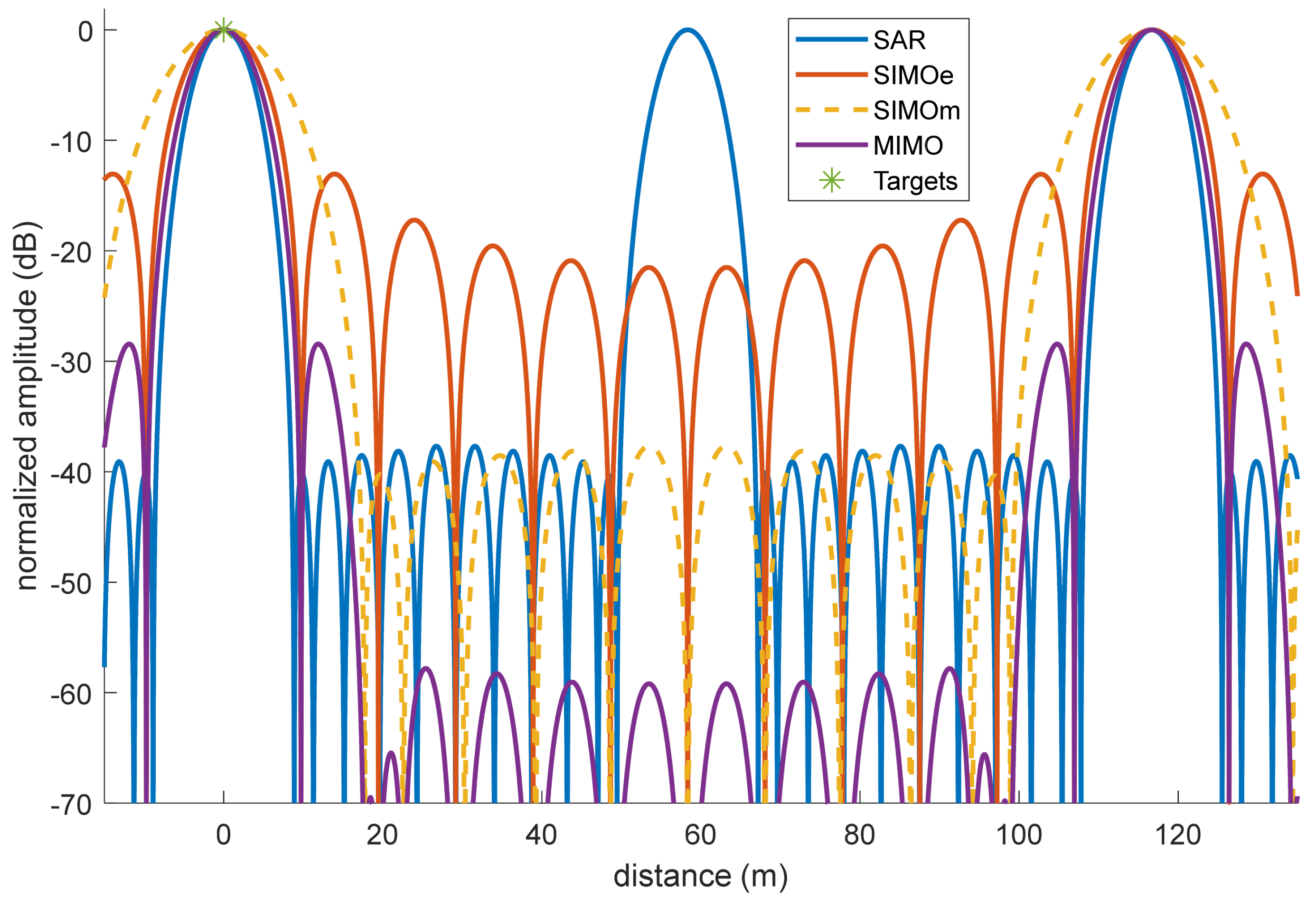
4.1. Comparison of SAR, SIMO, and MIMO Modes via Analytical Equations

The results shown in this section are generated using Equations (6), (11), and (15) by assuming that radar frequency is 1.2 GHz, the platforms’ mean altitude is 700 km and no windowing is applied. Tomographic aperture length, platform spacing, look angle, baseline tilt angle, and multi-static mode coefficient vary as needed to highlight how resolution and nearest ambiguity change as a function of these parameters.

Figure 12 shows the tomographic resolution along $\underset{\_}{n}$ (${\delta }_n$) vs. tomographic aperture length along $\underset{\_}{n}$ ($L_n$) for two different look angles and as a function of the multi-static mode. It is assumed that the baseline tilt angle ($\alpha$) is equal to look angle ($\theta$), which maximizes the perpendicular baseline for that look angle resulting in the best resolution for that platform distribution. Therefore, the perpendicular aperture lengths in the plots can also be considered as the actual aperture lengths.

As expected, longer aperture lengths are required to obtain finer resolutions. It can be seen that SAR mode has the best resolution in contrast with SIMO mode that shows the worst resolution performance. Furthermore, larger look angles (with same perpendicular baseline length) result in worse (coarser) resolution due to the longer slant range.

Figure 13 shows nearest ambiguity location along $\underset{\_}{n}$ ($A_n^1$) vs. platform spacing along $\underset{\_}{n}$ (${\mu }_n$) for two different look angles. It is assumed that the baseline tilt angle ($\alpha$) is equal to look angle ($\theta$). Therefore, the perpendicular platform spacings in the plots can also be considered as the actual platform spacings. The spacing among platforms is assumed to be equal (linear). No windowing is applied.

As expected, moving the nearest ambiguity further away requires smaller platform spacing. Smallest spacing is required for SAR mode, whereas the SIMO and MIMO modes yield the same spacing requirement. Smaller look angles require smaller spacing to obtain the same nearest ambiguity location due to shorter slant range. Note that, as shown by (13), the required nearest ambiguity location along $\underset{\_}{n}$ depends also on look angle in addition to local slope and maximum target height.

Based on (15), Figure 14 shows the minimum number of equally spaced platforms required for a specific tomographic resolution along $\underset{\_}{n}$ and the nearest ambiguity location along $\underset{\_}{n}$ for SAR, SIMO, and MIMO modes, both of which are independent of look angle. However, if the x-axes of the plots were the required vertical ambiguity location, then the required minimum number of platforms would be dependent on look angle and local slope. Resolution range is 2 to 30 m and nearest ambiguity location range is 20 to 100 m in the plots.

In general, more platforms are required for finer (smaller) resolution and larger nearest ambiguity location. For specific resolution and ambiguity location requirements, MIMO mode requires the least number of platforms (by a factor of ~0.7), whereas SAR and SIMO modes require equal number of platforms.

Based on (15), for specific $h_z^{max}$ and ${\delta }_n^{req}$, $N$ is larger for smaller $\theta$ and can be very large if $\theta \cong \epsilon$ provided that scene height (not antenna beam) is the limiting factor. Therefore, a larger $\theta$ and a large difference between $\theta$ and $\epsilon$ is advantageous to reduce the number of platforms. Interestingly, ${\delta }_n^{req}$ may also depend on $\theta$ (as illustrated in Figure 4) and even on $h_n^{max}$ if the minimum number of vertical layers (along $\underset{\_}{n}$) with a thickness of ${\delta }_n^{req}$ per target height is specified.

On the other hand, $N$ is independent of baseline tilt angle ($\alpha$). For a specific number of platforms, as the difference between $\theta$ and $\alpha$ increases, it would still be possible to meet both resolution and ambiguity requirements by increasing the spacing between the platforms. In fact, this may be useful if the spacing between platforms required to meet the ambiguity requirement cannot be achieved in practice (e.g., due to high collision risk), in which case increasing the difference between $\theta$ and $\alpha$ would be useful.

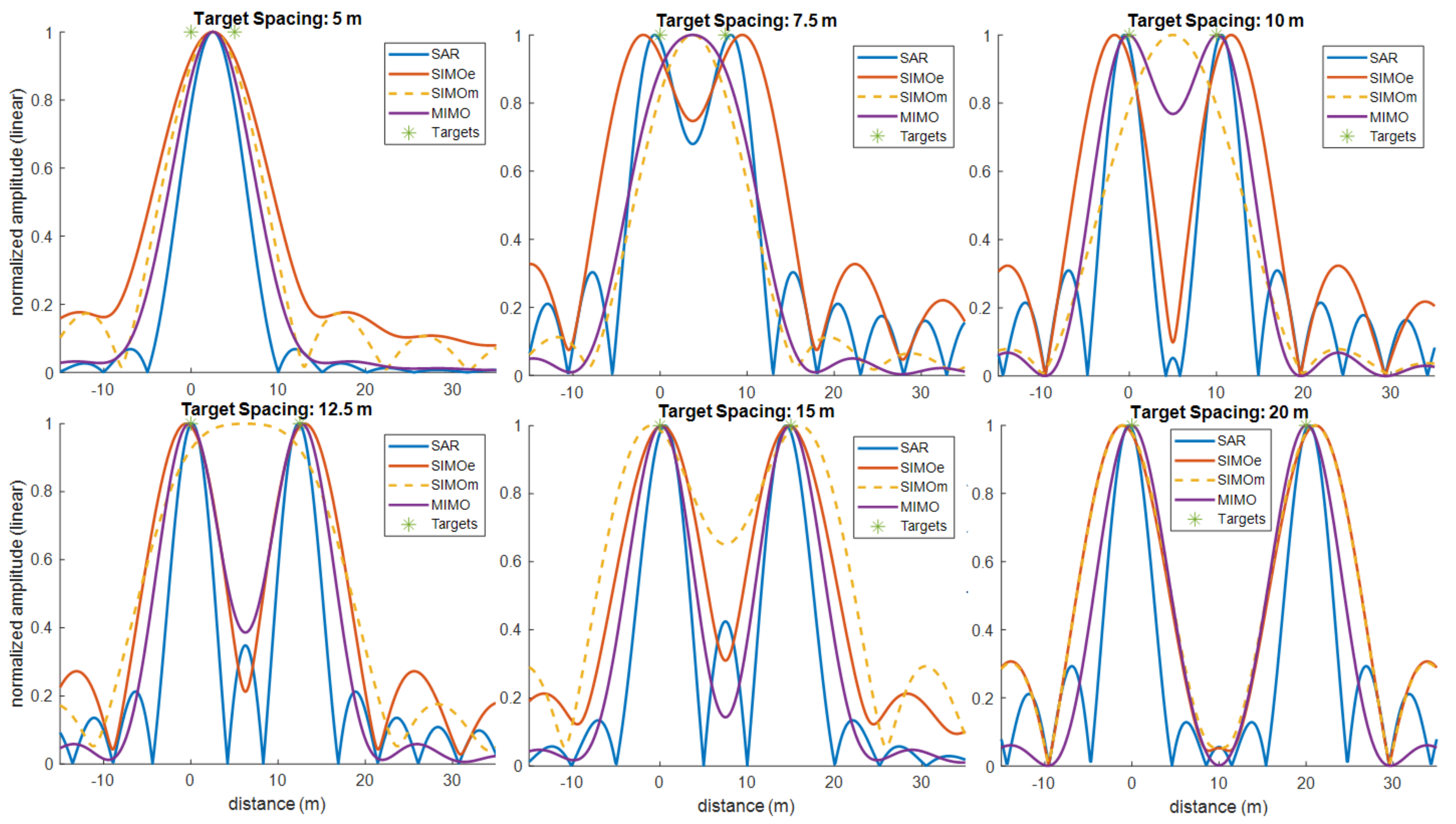
4.2. 1D Simulations

In this section, we present two example results from 1D simulations as described in Section 3 and shown in Figure 7 and Figure 8. The 1D raw data and the 1D tomographic images are generated using (16) and (17), respectively. Results with and without windowing are shown.

The first example is a point target at the origin which is directly below the center of tomographic aperture. Parameters used are given in

Table 1. Parameters used for the example 1D simulation.

Parameter	Value
Frequency	1.2 GHz
Altitude	700 km
Number of Targets	1
Number of Platforms	12
Tomographic Aperture	16.5 km
Platform Spacing	1500 m
Target Location	0 m
Scene Extend	150 m
Scene Resolution	1 cm

. The simulated image, shown in Figure 15, allows comparison of the tomographic resolution and ambiguities for the SAR, SIMO, and MIMO modes. For the SIMO mode, two options for transmit platform are shown: SIMOe (transmit platform is the 1st element at the edge) and SIMOm (transmit platform is the element in the middle). The performance for the configurations for which the transmit platform is neither the first platform nor the platform in the middle are expected to fall in between the performances of SIMOe and SIMOm. As expected, SAR mode gives the best resolution but the worst nearest ambiguity distance. MIMO mode result has the lowest sidelobes relative to the peak. Strong sidelobes can appear as fake weak targets and suppress actual weak targets at those locations.

It should be noted that, although the scene can be limited to avoid the ambiguity replicas, if there were targets at these locations (which is usually the case when imaging Earth’s surface) with sufficient antenna gain, their replicas would appear inside the scene of interest as ambiguous targets.

Each 1D plot is normalized to its peak. Note that the peak of MIMO mode is actually much larger than the peaks of the other two modes as MIMO integrates raw data from a larger number of transmit–receive platform pairs. This makes MIMO significantly more robust to random noise as it will be shown in Section 4.3 using 2D simulations.

The theoretical and measured resolutions (without windowing) and nearest ambiguity locations (along $\underset{\_}{n}$) are compared in

Table 2. Theoretical and measured tomographic resolutions and nearest ambiguity locations (along n).

	Theoretical Resolution		Measured Resolution		Theoretical Ambiguity Location	Measured Ambiguity Location	Measured PSLR
	Rayleigh	3.9 dB	Rayleigh	3.9 dB
SAR	4.9 m	4.9 m	4.9 m	4.9 m	58 m	58 m	−13 dB
SIMO	9.7 m	9.7 m	9.7 m	9.7 m	117 m	117 m	−13 dB
MIMO	9.7 m	7.0 m	9.7 m	7.0 m	117 m	117 m	−26 dB

. The theoretical resolutions are calculated using (2) for which the aperture length is taken as $L_n=N{\mu }_n=12\times 1.5=18$ km). Note that, although the SIMO and MIMO mode coefficients ($p_{\delta }$) in (7) have been derived empirically from simulations, this comparison shows that the 3.9 dB resolution calculated by the simulations and analytical equations agree for any specific combinations of input parameters as long as $N\ge ~5$ based on Figure 2. Measured peak sidelobe level ratios (PSLR) (without windowing) are also shown. It can be seen that, when the resolution and ambiguity coefficients for different modes as given in (7) and (12) are used, the measured resolution and ambiguity locations agree with the theoretical ones very well. The PSLRs (without windowing) for SAR and SIMO are −13 dB (which is the standard PSLR for a sinc function). Interestingly, the PSLR (without windowing) for MIMO is −26 dB which is a significant advantage.

Windowing can be applied along tomographic axis to reduce sidelobes at the cost of reduced processing gain and coarser resolution. For the above example, a Taylor window (nbar = 5) with sidelobe level set at −40 dB has been applied to the receive platforms. The normalized amplitude results are shown in Figure 16.

The changes in resolution, sidelobes, and gain depend on the window applied. The SNR loss for the window applied is 1.14 dB. The resolution and sidelobe levels with and without windowing are compared in

Table 3. Measured tomographic resolutions and sidelobe levels with and without windowing.

	Resolution along Elevation $\left(\underset{\_}{\mathit{n}}\right)$				PSLR
	No Window		Taylor Window (−40 dB, nbar = 5)		No Window	Taylor Window (−40 dB, nbar = 5)
	Rayleigh	3.9 dB	Rayleigh	3.9 dB
SAR	4.9 m	4.9 m	17.7 m	6.9 m	−13 dB	−38 dB
SIMOe	9.7 m	9.7 m	19.4 m	9.7 m	−13 dB	−13 dB
SIMOm	9.7 m	9.7 m	35.4 m	13.7 m	−13 dB	−38 dB
MIMO	9.7 m	7.0 m	19.4 m	8.1 m	−26 dB	−28 dB

. It is observed that the 3.9 dB resolutions for the SAR and SIMOm modes increase (become coarser) significantly, the resolution for the SIMOe mode does not change, and the resolution for the MIMO mode increases slightly. On the other hand, although all sidelobe levels go down to −40 dB for the SAR and SIMOm modes, they do not change for the SIMOe mode. For the MIMO mode, the PSLR goes down by only a few dB, but the far sidelobes (which were already below −40 dB without windowing) are further reduced to approximately −60 dB.

The second example illustrates the ability of each mode in resolving two-point targets (which can represent two dominant scatterers in a scene) separated by various distances (5–20 m). The parameters are the same as in Table 1, except for the target positions and scene size. No windowing is applied.

For this case, an example simulated complex 1D raw data for the SAR, SIMO, and MIMO modes are shown in Figure 17. Even though both the platform and target distributions are in 1D, the MIMO raw data space is shown in 2D with the two axes representing the transmit and receive platforms and the color representing the amplitude or phase. The relation of SAR and SIMO raw data to the MIMO is indicated by red lines.

The processed 1D tomograms are shown in Figure 18. The positions and relative reflectivities of the two targets are also shown. The reflectivities of the two targets are assumed equal. Linear scale is used to better illustrate the discrimination of two targets.

It can be seen that the locations and reflectivities of the targets agree with the peaks in the simulation results as long as the targets are sufficiently separated; otherwise, the two mainlobes start to merge due to insufficient resolution. Depending on the relative intensities, distances, and phases of the two mainlobes (which determine whether the two peaks merge coherently or incoherently), two sharper peaks or a single broad peak in between the two targets can appear, as demonstrated. Apparently, the ability to distinguish two targets depends not only on the distance between the two, but also on the tomographic mode. It can be observed that a distance of approximately twice the 3–4 dB resolution for the SAR, SIMOm, and MIMO modes is required to ensure that the two peaks are clearly visible. Interestingly, for SIMOe, a distance equal to resolution seems to be sufficient, whereas for SIMOm, a distance of twice the resolution seems to be required. This gives SIMOe as good resolving capability as the SAR mode which benefits from the two-way phase shift. In general, the resolving capability of the SAR mode is similar to SIMOe, which is better than MIMO, which is better than SIMOm. SIMOe offers larger baseline diversity and its maximum baseline is twice the maximum baseline of SIMOm making it sensible that SIMOe has better capability to discriminate two targets than SIMOm which has the worst resolving capability among the four modes. On the other hand, sidelobes are not reduced with windowing in SIMOe whereas they can be significantly reduced in the SIMOm mode at the expanse of resolution. These conclusions are valid regardless of the choice of the simulation parameters.

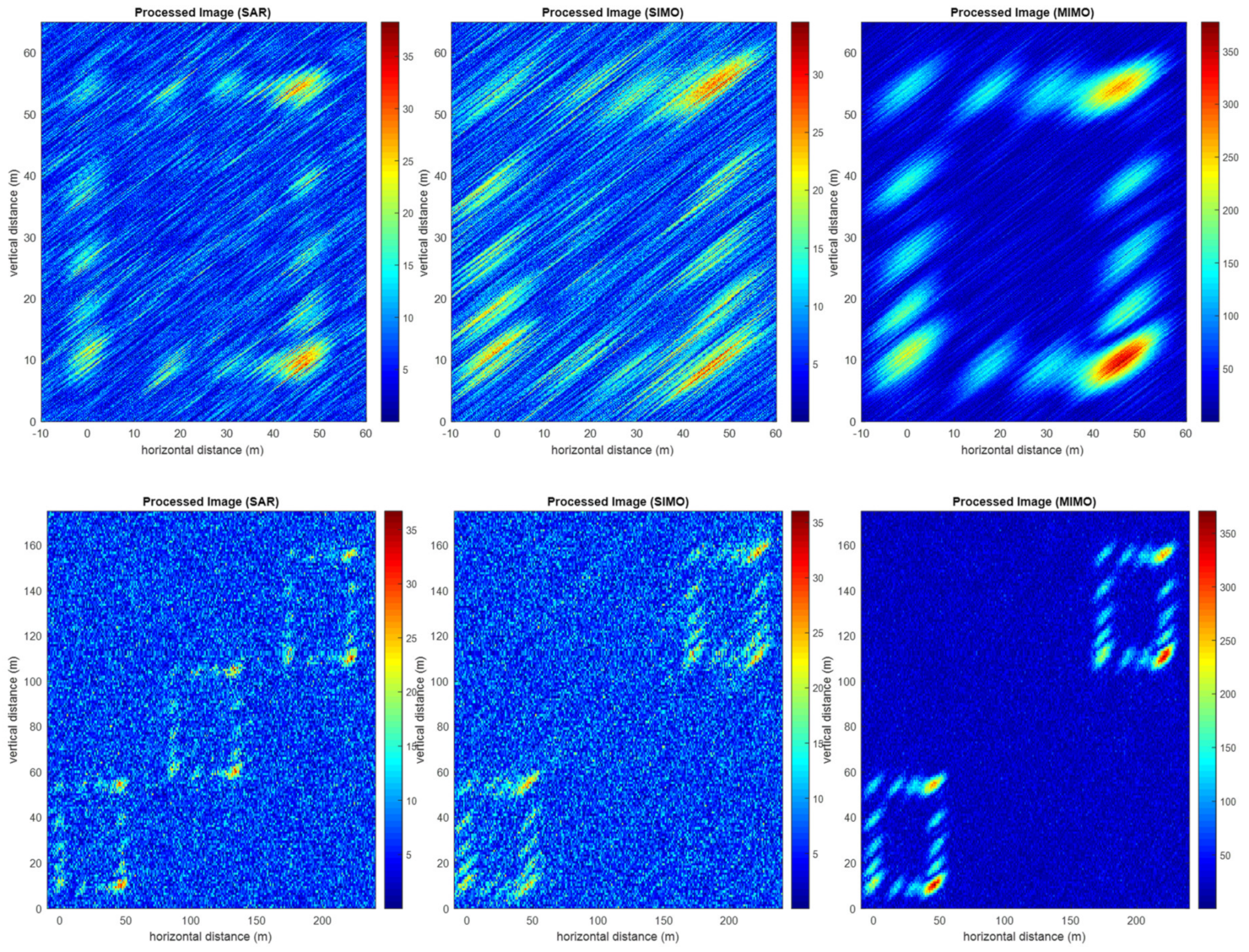
4.3. 2D Simulations

In this section, we present and compare several tomograms obtained from simulations when platform and target distributions are both in 2D as shown in Figure 9 and Figure 11, respectively. The 2D raw data and the 2D tomographic images are generated using (18) and (19), respectively. No windowing is applied. Results for different geometries (look angle, baseline tilt, altitude, and platform distributions) as well as using different radar parameters (frequency, bandwidth, SNR, and PRI) are shown. For each example, values of relevant parameters are listed and the observation geometry is illustrated. For all examples, the same target distribution (shown in Figure 19) is used as input to the raw data generation. This distribution includes varying distances among targets (3–18 m horizontally and 3–15 m vertically) which is useful to analyze resolution performance. The reflectivities of all point targets are assumed to be equal. For the SIMO mode, only SIMOe configuration is considered as SIMOe offers better target discrimination capability than SIMOm as was demonstrated in Section 4.2.

An example raw data amplitude for 2D simulations is shown in Figure 20. It should be noted that range compression (i.e., matched filter output) is included in the raw data shown. The range migration over the tomographic aperture is evident.

Images are shown for SAR/SIMOe/MIMO modes and in linear amplitude. Small scene extent (of focused image) is useful to illustrate resolution, whereas large scene extent is useful to illustrate ambiguities. Therefore, for most of the examples, two sets of images are shown: one with fine image resolution (pixel spacing of focused image) but small scene extent (so that details are more visible and simulation runs faster) and another one with large scene extent (to illustrate ambiguities if any) but coarse resolution (so that simulation runs faster). For fine resolution, 20 cm is used, and for coarse resolution, 1 m is used. Scene size varies from example to example. The changed parameters with respect to Example 1 are highlighted in red/italic font in the tables. The SNRs listed in the tables include only random additive noise and represents the SNR of a single platform (before tomographic processing gain).

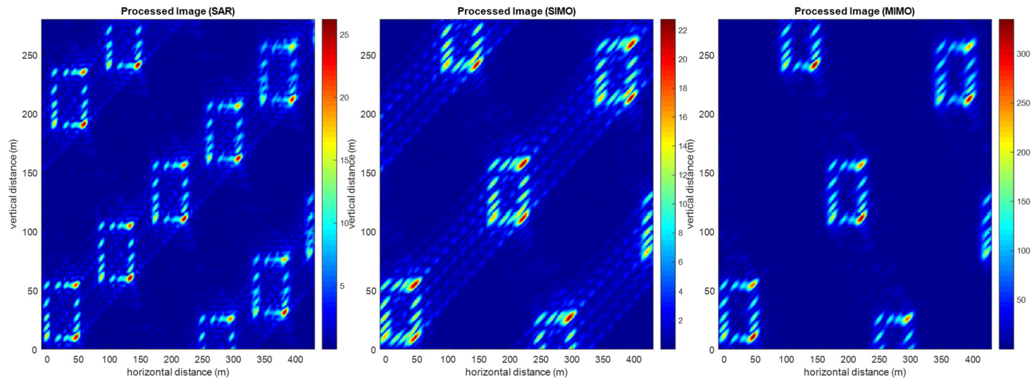
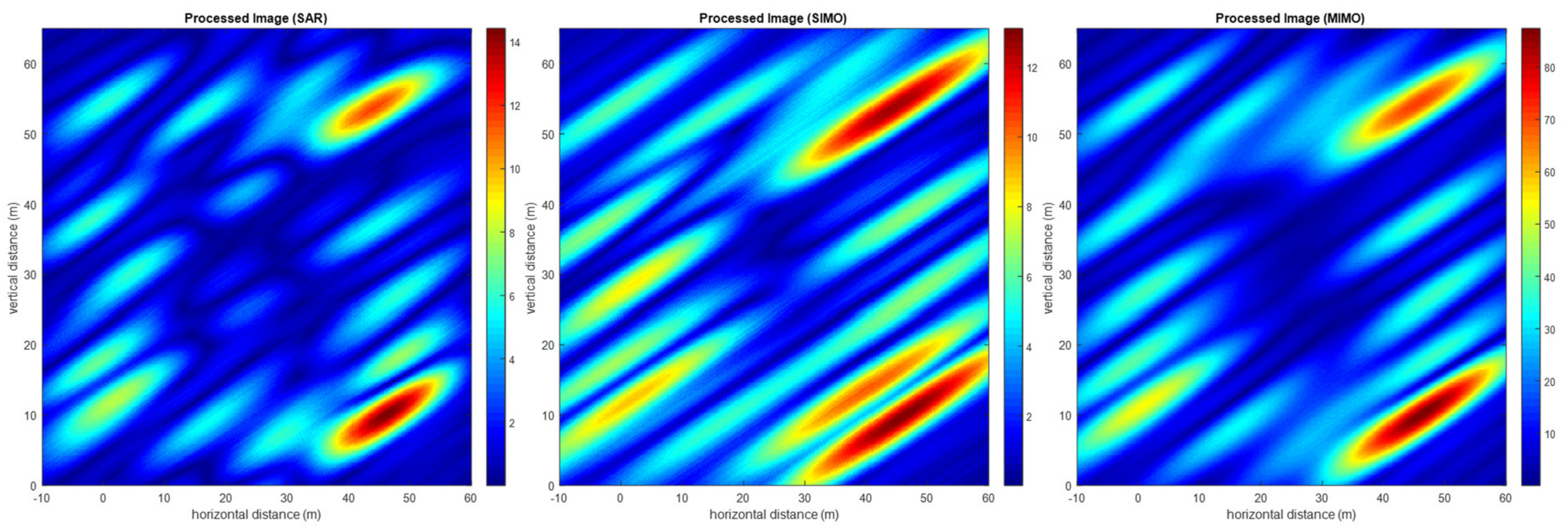
4.3.1. Example 1: Reference Scenario

For Example 1, the input parameters are given in

Table 4. Parameters used for Example 1.

Parameter	Value
Frequency	1.2 GHz
Bandwidth	40 MHz
Pulse Width	10 us
PRI	100 us
Altitude	700 km
Number of Platforms	12
Tomographic Aperture	11 km
Platform Spacing	1 km
Baseline Tilt	30°
Look Angle	30°
SNR	50 dB

, the observation geometry is shown in Figure 21, and the simulated 2D images are shown in Figure 22.

4.3.2. Example 2: Changing SNR

For Example 2, the input parameters are given in

Table 5. Parameters used for Example 2.

Parameter	Value
Frequency	1.2 GHz
Bandwidth	40 MHz
Pulse Width	10 us
PRI	100 us
Altitude	700 km
Number of Platforms	12
Tomographic Aperture	11 km
Platform Spacing	1 km
Baseline Tilt	30°
Look Angle	30°
SNR	20 dB

and the simulated 2D images are shown in Figure 23. The observation geometry is the same with Example 1.

4.3.3. Example 3: Changing Frequency and Bandwidth

For Example 3, the input parameters are given in

Table 6. Parameters used for Example 3.

Parameter	Value
Frequency	0.6 GHz
Bandwidth	20 MHz
Pulse Width	10 us
PRI	100 us
Altitude	700 km
Number of Platforms	12
Tomographic Aperture	11 km
Platform Spacing	1 km
Baseline Tilt	30°
Look Angle	30°
SNR	50 dB

and the simulated 2D images are shown in Figure 24. The observation geometry is the same with Example 1.

4.3.4. Example 4: Changing PRI and Pulse Width

For Example 4, the input parameters are given in

Table 7. Parameters used for Example 4.

Parameter	Value
Frequency	1.2 GHz
Bandwidth	40 MHz
Pulse Width	0.5 us
PRI	1 us
Altitude	700 km
Number of Platforms	12
Tomographic Aperture	11 km
Platform Spacing	1 km
Baseline Tilt	30°
Look Angle	30°
SNR	50 dB

and the simulated 2D images are shown in Figure 25. The observation geometry is the same with Example 1.

This example illustrates the ambiguities along $\underset{\_}{r}$ and the coupling of ambiguities along $\underset{\_}{r}$ and along $\underset{\_}{n}$. As the scene sizes in our examples are relatively small, the range replicas fall outside the scene of interest. However, there can be other targets at the location of those replicas (either due to local slope or due to double replicas falling on the surface). Here, instead of having to simulate a very large scene, the PRI (and therefore pulse width) is decreased to move the replicas along r much closer to the scene of interest.

4.3.5. Example 5: Changing Altitude

For Example 5, the input parameters are given in

Table 8. Parameters used for Example 5.

Parameter	Value
Frequency	1.2 GHz
Bandwidth	40 MHz
Pulse Width	10 us
PRI	100 us
Altitude	400 km
Number of Platforms	12
Tomographic Aperture	11 km
Platform Spacing	1 km
Baseline Tilt	30°
Look Angle	30°
SNR	50 dB

and the simulated 2D images are shown in Figure 26. Although the altitude is different, the observation geometry (platform distribution and look direction) is the same with Example 1.

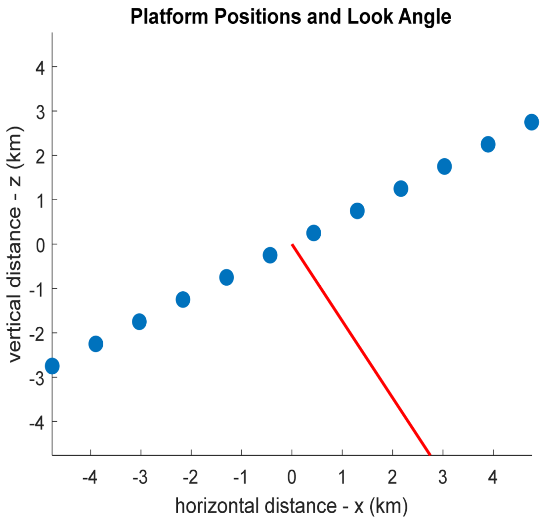
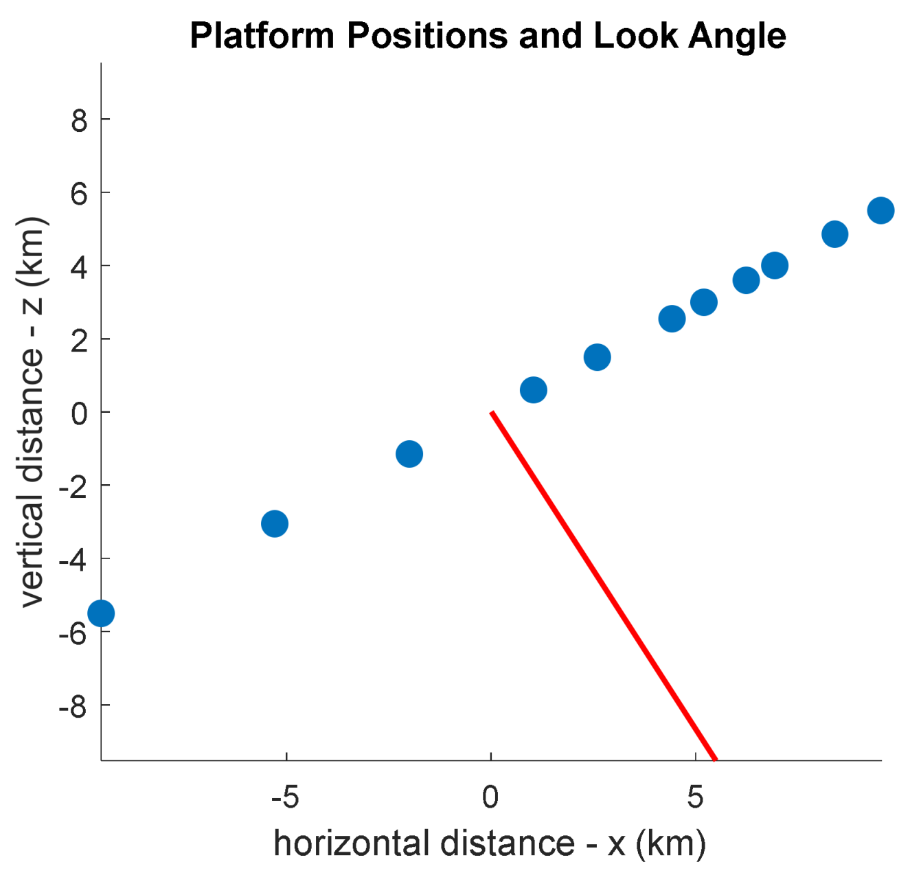
4.3.6. Example 6: Changing Baseline Tilt and Look Angle

For Example 6, the input parameters are given in

Table 9. Parameters used for Example 6.

Parameter	Value
Frequency	1.2 GHz
Bandwidth	40 MHz
Pulse Width	10 us
PRI	100 us
Altitude	700 km
Number of Platforms	12
Tomographic Aperture	11 km
Platform Spacing	1 km
Baseline Tilt	50°
Look Angle	50°
SNR	50 dB

, the observation geometry is shown in Figure 27, and the simulated 2D images are shown in Figure 28.

4.3.7. Example 7: Changing Number of Platforms and Tomographic Aperture

For Example 7, the input parameters are given in

Table 10. Parameters used for Example 7.

Parameter	Value
Frequency	1.2 GHz
Bandwidth	40 MHz
Pulse Width	10 us
PRI	100 us
Altitude	700 km
Number of Platforms	6
Tomographic Aperture	5 km
Platform Spacing	1 km
Baseline Tilt	30°
Look Angle	30°
SNR	50 dB

, the observation geometry is shown in Figure 29, and the simulated 2D images are shown in Figure 30.

4.3.8. Example 8: Changing Tomographic Aperture and Platform Spacing (Equal Spacing)

For Example 8, the input parameters are given in

Table 11. Parameters used for Example 8.

Parameter	Value
Frequency	1.2 GHz
Bandwidth	40 MHz
Pulse Width	10 us
PRI	100 us
Altitude	700 km
Number of Platforms	12
Tomographic Aperture	22 km
Platform Spacing	2 km
Baseline Tilt	30°
Look Angle	30°
SNR	50 dB

, the observation geometry is shown in Figure 31, and the simulated 2D images are shown in Figure 32.

4.3.9. Example 9: Changing Tomographic Aperture and Platform Spacing (Unequal Spacing)

For Example 9, the input parameters are given in

Table 12. Parameters used for Example 9.

Parameter	Value
Frequency	1.2 GHz
Bandwidth	40 MHz
Pulse Width	10 us
PRI	100 us
Altitude	700 km
Number of Platforms	12
Tomographic Aperture	22 km
Platform Spacing	variable
Baseline Tilt	30°
Look Angle	30°
SNR	50 dB

, the observation geometry is shown in Figure 33, and the simulated 2D images are shown in Figure 34.

5. Discussion

The results reported in Section 4 highlight several aspects of how SAR tomograms change with formation geometry, radar parameters, scene characteristics, and tomographic modes.

A peculiarity of tomographic imaging is the tilted resolution cell, which implies that the vertical and horizontal target resolving capabilities depend not only on tomographic resolution itself, but also on range resolution, look angle, and orientation of point targets relative to each other. Overall, the target resolving capability of SAR mode is better than that of MIMO mode, which in turn is better than that of SIMO mode.

The tomographic ambiguity replicas along $\underset{\_}{n}$ of SAR are worse (closer to scene) than those of SIMO and MIMO. SIMO and MIMO reveal the same performance in terms of tomographic ambiguities. As tomographic ambiguities along $\underset{\_}{n}$ occur at different heights due to non-zero look angle, they would not cause issues unless there are targets at those heights, which may occur especially when the local slope is not significantly less than the look angle. In other words, having a sufficiently large difference between look angle and terrain slope makes it possible to tolerate tomographic ambiguity replicas at closer distances. Ambiguities also occur along $\underset{\_}{r}$ usually at larger distances compared to the ones along $\underset{\_}{n}$. Ambiguities along $\underset{\_}{n}$ and along $\underset{\_}{r}$ are coupled, i.e., replicas along $\underset{\_}{n}$ also have replicas along $\underset{\_}{r}$, and vice versa. Tomographic processing helps eliminate ambiguities along $\underset{\_}{r}$ because they appear at large heights and there would be no targets at those heights unless the local slope is steep over a large distance. However, double replicas (coupled along $\underset{\_}{n}$ and $\underset{\_}{r}$) can still fall onto the near surface which are usually illuminated by the antenna sidelobes causing relatively weak ambiguities. This can be avoided by having sufficient gap between the tomographic ambiguities or by having low antenna gains at corresponding angles.

The tomographic sidelobes of MIMO are significantly better (lower) than those of SAR and SIMO, which means lower multiplicative noise (i.e., lower clutter-to-signal and ambiguity-to-signal ratios). For equal platform spacing, tomographic sidelobes can be reduced by windowing (except for SIMOe) at the expense of tomographic resolution and processing gain. As tomographic sidelobes occur along stripes aligned along $\underset{\_}{n}$, only the near sidelobes fall onto the region limited by target heights. However, for larger local slopes, sidelobes at further distance can coincide with other targets.

Assuming fixed number of platforms and constant SNR per platform, MIMO has much better SNR (after processing) than SAR and SIMO due to its processing gain being twice (in dB scale) of the other two modes. Noise samples in two neighboring pixels whose time separation is less than half of the sampling time resolution of the simulation are assumed perfectly correlated in the simulations. Time separation of two targets is much less if targets are aligned along $\underset{\_}{n}$. Therefore, random noise appears in the tomographic images with high pixel resolution as line segments tilted along $\underset{\_}{n}$.

Although lower radar frequency is better for foliage penetration and brings the benefit of moving the ambiguities further away, lower frequency results in coarser tomographic resolution and (as lower frequency usually means lower bandwidth) also coarser range resolution, which in turn may affect vertical and horizontal resolutions as discussed in Section 2.1. Furthermore, size, weight, and power consumption of radar hardware are usually larger for lower frequencies.

Higher SNR and better tomographic (as well as along-track) resolution can be obtained by lowering the altitudes of the multi-static formation. However, ambiguities move closer and, at low altitudes, it is costlier to maintain satellite trajectory.

The tomographic ambiguities can be moved to further distances by increasing the look angle (due to longer range) which also tilts the ambiguity axis so that larger target heights and larger surface slopes can be tolerated. However, this leads to lower SNR and worse tomographic (as well as along-track) resolution due to longer range. Furthermore, the resolution cell tilts further and, assuming the more common case ${\delta }_{r}cos\theta <{\delta }_{n}sin\theta$, horizontal resolution becomes finer while vertical resolution becomes coarser.

In terms of tomographic baseline, platform spacing, and number of platforms, the following conclusions can be drawn:

• Larger baseline, same spacing results in same ambiguity, better resolution, more platforms.
• Same baseline, larger spacing results in worse ambiguity, same resolution, less platforms.
• Larger baseline, larger spacing results in worse ambiguity, better resolution, same number of platforms
• Smaller baseline, smaller spacing results in better ambiguity, worse resolution, same number of platforms

Unequal spacing smears out the ambiguity replicas at the cost of increased sidelobes. MIMO, which has the lowest sidelobes among the three modes, can better tolerate such increase in sidelobes as compared to SAR and SIMO. In addition to higher SNR, when combined with nonlinear spacing, the MIMO mode allows reasonable tomographic resolution and ambiguity performance with fewer platforms than SAR and SIMO.

In terms of tomographic performance vs. hardware requirements and design complexity, the results in Section 4 leads to the following guidelines:

• SAR has the best resolution but the worst ambiguity performance. In addition, it has lower SNR and higher sidelobes than MIMO. Similar to MIMO, SAR requires all platforms to have TX capability. However, unlike MIMO, SAR does not require clock synchronization as each platform receives its own signal. SAR requires less data size than MIMO.
• SIMO has better ambiguity performance than SAR but the worst resolution performance. Nevertheless, SIMOe has as good target resolving capability as SAR (even though its resolution is worse than SAR). On the other hand, SIMOm has the worst resolving capability. In addition, SIMO has lower SNR and higher sidelobes than MIMO. To its advantage, SIMO requires only one platform with TX capability which translates into lower costs. Furthermore, TX/RX timing and clock synchronization are less challenging in SIMO than MIMO. SIMO requires less data size than MIMO.
• MIMO has the best overall performance in terms of tomographic SNR, resolution, ambiguity, and sidelobes. Even though its resolution is not the best, it is superior in terms of SNR and sidelobes. Its ambiguities can also be reduced by nonlinear platform spacing at the expense of sidelobes since it can tolerate higher sidelobes. However, MIMO requires all platforms to have TX capability as well as clock synchronization among platforms to synchronize timing and preserve phase coherence both of which translate into higher costs. MIMO also requires either orthogonal codes to be able to transmit simultaneously or more complex TX/RX timing to avoid eclipsing of multiple TX/RX pulses. Moreover, MIMO data (before tomographic processing) require significantly larger data size (depending on the number of platforms), which poses requirements on downlink capacity and/or onboard processing.

6. Conclusions

Multi-static radar formations enable the implementation of single-pass TomoSAR technique from space to resolve the vertical structure of volumetric media, such as vegetation and ice. Designing TomoSAR formations requires exploring a trade space consisting of parameters related to platform distribution, observation geometry, multi-static transmit/receive mode, and radar instrument. In this paper, we examined the quality of the expected tomograms under several scenarios by varying the characteristics of the multi-static formation using analytical expressions as well as numerical simulations. Tomogram quality was assessed in terms of resolution, ambiguity location, sidelobes, and SNR. In particular, the performances of three major multi-static modes—SAR, SIMO and MIMO—have been intercompared with the aim to identify and quantify pros and cons of each mode. The MIMO mode offers the best overall performance at the expense of increased system complexity. The SAR mode gives the best resolution but the worst ambiguity level. The SIMO mode shows improved ambiguity level with respect to SAR mode but gives the worst resolution performance. Our simulation approach has been intentionally simplistic in order to provide an effective tool to guide the first-order design of airborne and spaceborne TomoSAR missions. Only simplified spaceborne scenarios were considered here, leaving the airborne cases to future analyses. We intentionally avoided giving recommendations on the optimal number of baselines and multi-static modes as they flow down from science requirements and depend on other system aspects (e.g., realistic orbits) that fall outside of the scope of this work. We also limited the tomographic processing to the time-domain back-projection algorithm given its robustness and straightforward implementation, but other algorithms such as Capon or compressive sensing could be applied to simulated data, which may lead to different quality metrics results. Future works may also include the effect of antenna pattern, the along-track dimension, error sources other than noise and ambiguity, increasing the fidelity of the simulated scene (e.g., by incorporating scattering dependent on look angle or temporal decorrelation), as well as the complexity of the formation geometry (e.g., using realistic orbits and platform distributions) as a function of the specific application domain (forestry, agriculture, urban, etc.). However, adding simulation complexity will also increase the dimension of the trade space, potentially making it more challenging to evaluate the optimal TomoSAR formations and relevant radar parameters.

References

- Jordan, R. The Seasat-A synthetic aperture radar system. IEEE J. Ocean. Eng. 1980, 5, 154–164. [Google Scholar] [CrossRef]
- Rosen, P.A.; Hensley, S.; Joughin, I.R.; Li, F.K.; Madsen, S.N.; Rodriguez, E.; Goldstein, R.M. Synthetic aperture radar interferometry. Proc. IEEE 2000, 88, 333–380. [Google Scholar] [CrossRef]
- Ferretti, A.; Prati, C.; Rocca, F. Permanent scatterers in SAR interferometry. IEEE Trans. Geosci. Remote Sens. 2001, 39, 8–20. [Google Scholar] [CrossRef]
- Massonnet, D.; Rossi, M.; Carmona, C.; Adragna, F.; Peltzer, G.; Feigl, K.; Rabaute, T. The displacement field of the Landers earthquake mapped by radar interferometry. Nature 1993, 364, 138–142. [Google Scholar] [CrossRef]
- Bamler, P.H.R. Synthetic Aperture Radar Interferometry. Inverse Probl. 1998, 14, 1–54. [Google Scholar] [CrossRef]
- Gini, F.; Lombardini, F.; Montanari, M. Layover solution in multibaseline SAR interferometry. IEEE Trans. Aerosp. Electron. Syst. 2002, 38, 1344–1356. [Google Scholar] [CrossRef]
- Reigber, A.; Moreira, A. First demonstration of airborne SAR tomography using multibaseline L-band data. IEEE Trans. Geosci. Remote Sens. 2000, 38, 2142–2152. [Google Scholar] [CrossRef]
- Moreira, A.; Prats-Iraola, P.; Younis, M.; Krieger, G.; Hajnsek, I.; Papathanassiou, K.P. A tutorial on synthetic aperture radar. IEEE Geosci. Remote Sens. Mag. 2013, 1, 6–43. [Google Scholar] [CrossRef] [Green Version]
- Lombardini, F.; Montanari, M.; Gini, F. Reflectivity estimation for multibaseline interferometric radar imaging of layover extended sources. IEEE Trans. Signal Process. 2003, 51, 1508–1519. [Google Scholar] [CrossRef]
- Fornaro, G.; Serafino, F.; Soldovieri, F. Three-dimensional focusing with multipass SAR data. IEEE Trans. Geosci. Remote Sens. 2003, 41, 507–517. [Google Scholar] [CrossRef]
- Pasquali, P.; Prati, C.; Rocca, F.; Seymour, M.; Fortuny, J.; Ohlmer, E.; Sieber, A. A 3-D SAR experiment with EMSL data. In Proceedings of the 1995 International Geoscience and Remote Sensing Symposium, IGARSS ’Quantitative Remote Sensing for Science and Applications, Firenze, Italy, 10–14 July 1995; Volume 1, pp. 784–786. [Google Scholar]
- Farhat, N.H.; Werner, C.L.; Chu, T.H. Prospects for three-dimensional projective and tomographic imaging radar networks. Radio Sci. 1984, 19, 1347–1355. [Google Scholar] [CrossRef]
- Homer, J.; Longstaff, I.; Callaghan, G. High resolution 3-D SAR via multi-baseline interferometry. In Proceedings of the IGARSS ’96. 1996 International Geoscience and Remote Sensing Symposium, Lincoln, NE, USA, 31 May 1996; IEEE: New York, NY, USA, 2002. [Google Scholar]
- Aghababaee, H.; Ferraioli, G.; Ferro-Famil, L.; Huang, Y.; D’Alessandro, M.M.; Pascazio, V.; Schirinzi, G.; Tebaldini, S. Forest SAR Tomography: Principles and Applications. IEEE Geosci. Remote Sens. Mag. 2020, 8, 30–45. [Google Scholar] [CrossRef]
- Tebaldini, S. Single and Multipolarimetric SAR Tomography of Forested Areas: A Parametric Approach. IEEE Trans. Geosci. Remote Sens. 2010, 48, 2375–2387. [Google Scholar] [CrossRef]
- Minh, D.H.T.; Le Toan, T.; Rocca, F.; Tebaldini, S.; D’Alessandro, M.M.; Villard, L. Relating P-Band Synthetic Aperture Radar Tomography to Tropical Forest Biomass. IEEE Trans. Geosci. Remote Sens. 2013, 52, 967–979. [Google Scholar] [CrossRef]
- Pardini, M.; Tello, M.; Cazcarra-Bes, V.; Papathanassiou, K.P.; Hajnsek, I. L- and P-Band 3-D SAR Reflectivity Profiles versus Lidar Waveforms: The AfriSAR Case. IEEE J. Sel. Top. Appl. Earth Obs. Remote Sens. 2018, 11, 3386–3401. [Google Scholar] [CrossRef]
- Frey, O.; Meier, E. 3-D Time-Domain SAR Imaging of a Forest Using Airborne Multibaseline Data at L- and P-Bands. IEEE Trans. Geosci. Remote Sens. 2011, 49, 3660–3664. [Google Scholar] [CrossRef]
- Yu, Y.; D’Alessandro, M.M.; Tebaldini, S.; Liao, M. Signal Processing Options for High Resolution SAR Tomography of Natural Scenarios. Remote Sens. 2020, 12, 10. [Google Scholar]
- Huang, Y.; Ferro-Famil, L.; Reigber, A. Under-Foliage Object Imaging Using SAR Tomography and Polarimetric Spectral Estimators. IEEE Trans. Geosci. Remote Sens. 2011, 50, 2213–2225. [Google Scholar] [CrossRef] [Green Version]
- Cazcarra-Bes, V.; Pardini, M.; Tello, M.; Papathanassiou, K.P. Comparison of Tomographic SAR Reflectivity Reconstruction Algorithms for Forest Applications at L-band. IEEE Trans. Geosci. Remote Sens. 2019, 58, 147–164. [Google Scholar] [CrossRef]
- Aguilera, E.; Nannini, M.; Reigber, A. A Data-Adaptive Compressed Sensing Approach to Polarimetric SAR Tomography of Forested Areas. IEEE Geosci. Remote Sens. Lett. 2012, 10, 543–547. [Google Scholar] [CrossRef]
- Joerg, H.; Pardini, M.; Hajnsek, I.; Papathanassiou, K.P. 3-D Scattering Characterization of Agricultural Crops at C-Band Using SAR Tomography. IEEE Trans. Geosci. Remote Sens. 2018, 56, 3976–3989. [Google Scholar] [CrossRef]
- Lombardini, F. Differential tomography: A new framework for SAR interferometry. IEEE Trans. Geosci. Remote Sens. 2004, 43, 37–44. [Google Scholar] [CrossRef]
- Lombardini, F.; Pardini, M. Superresolution Differential Tomography: Experiments on Identification of Multiple Scatterers in Spaceborne SAR Data. IEEE Trans. Geosci. Remote Sens. 2011, 50, 1117–1129. [Google Scholar] [CrossRef]
- Pauciullo, A.; Reale, D.; De Maio, A.; Fornaro, G. Detection of Double Scatterers in SAR Tomography. IEEE Trans. Geosci. Remote Sens. 2012, 50, 3567–3586. [Google Scholar] [CrossRef]
- Zhu, X.X.; Bamler, R. Let’s Do the Time Warp: Multicomponent Nonlinear Motion Estimation in Differential SAR Tomography. IEEE Geosci. Remote Sens. Lett. 2011, 8, 735–739. [Google Scholar] [CrossRef] [Green Version]
- Siddique, M.A.; Wegmüller, U.; Hajnsek, I.; Frey, O. Single-Look SAR Tomography as an Add-On to PSI for Improved Deformation Analysis in Urban Areas. IEEE Trans. Geosci. Remote Sens. 2016, 54, 6119–6137. [Google Scholar] [CrossRef]
- Budillon, A.; Diaz-Fuentes, G. GLRT Based on Support Estimation for Multiple Scatterers Detection in SAR Tomography. IEEE J. Sel. Top. Appl. Earth Obs. Remote Sens. 2015, 9, 1086–1094. [Google Scholar] [CrossRef]
- Banda, F.; Dall, J.; Tebaldini, S. Single and Multipolarimetric P-Band SAR Tomography of Subsurface Ice Structure. IEEE Trans. Geosci. Remote Sens. 2015, 54, 2832–2845. [Google Scholar] [CrossRef]
- Rekioua, B.; Davy, M.; Ferro-Famil, L.; Tebaldini, S. Snowpack permittivity profile retrieval from tomographic SAR data. Comptes Rendus Phys. 2017, 18, 57–65. [Google Scholar] [CrossRef]
- Xu, X.; Baldi, C.A.; De Bleser, J.-W.; Lei, Y.; Yueh, S.; Esteban-Fernandez, D. Multi-Frequency Tomography Radar Observations of Snow Stratigraphy at Fraser During SnowEx. In Proceedings of the IGARSS 2018—2018 IEEE International Geoscience and Remote Sensing Symposium, Valencia, Spain, 22–27 July 2018; IEEE: New York, NY, USA, 2018; pp. 6269–6272. [Google Scholar]
- Frey, O.; Werner, C.L.; Wiesmann, A. Tomographic profiling of the structure of a snow pack at X-/Ku-Band using SnowScat in SAR mode. In Proceedings of the 2015 European Radar Conference (EuRAD), Paris, France, 9–11 September 2015; IEEE: New York, NY, USA, 2015; pp. 21–24. [Google Scholar]
- Morrison, K.; Bennett, J. Tomographic Profiling—A Technique for Multi-Incidence-Angle Retrieval of the Vertical SAR Backscattering Profiles of Biogeophysical Targets. IEEE Trans. Geosci. Remote Sens. 2013, 52, 1350–1355. [Google Scholar] [CrossRef]
- Frey, O.; Werner, C.L.; Caduff, R.; Wiesmann, A. Tomographic Profiling with Snowscat within the ESA Snowlab Campaign: Time Series of Snow Profiles Over three Snow Seasons. In Proceedings of the IGARSS 2018—2018 IEEE International Geoscience and Remote Sensing Symposium, Valencia, Spain, 22–27 July 2018; IEEE: New York, NY, USA, 2018; pp. 6512–6515. [Google Scholar]
- Frey, O.; Meier, E. Analyzing Tomographic SAR Data of a Forest with Respect to Frequency, Polarization, and Focusing Technique. IEEE Trans. Geosci. Remote Sens. 2011, 49, 3648–3659. [Google Scholar] [CrossRef] [Green Version]
- Tebaldini, S.; Rocca, F. Multibaseline Polarimetric SAR Tomography of a Boreal Forest at P- and L-Bands. IEEE Trans. Geosci. Remote Sens. 2011, 50, 232–246. [Google Scholar] [CrossRef]
- Ulander, L.M.H.; Monteith, A.R.; Soja, M.J.; Eriksson, L.E.B. Multiport Vector Network Analyzer Radar for Tomographic Forest Scattering Measurements. IEEE Geosci. Remote Sens. Lett. 2018, 15, 1897–1901. [Google Scholar] [CrossRef]
- Lavalle, M.; Hawkins, B.; Hensley, S. Tomographic imaging with UAVSAR: Current status and new results from the 2016 AfriSAR campaign. In Proceedings of the 2017 IEEE International Geoscience and Remote Sensing Symposium (IGARSS), Fort Worth, TX, USA, 23–28 July 2017; IEEE: New York, NY, USA, 2017; pp. 2485–2488. [Google Scholar]
- Khati, U.; LaValle, M.; Singh, G. Spaceborne tomography of multi-species Indian tropical forests. Remote Sens. Environ. 2019, 229, 193–212. [Google Scholar] [CrossRef]
- Cloude, S.R. Polarization coherence tomography. Radio Sci. 2006, 41. [Google Scholar] [CrossRef]
- Capon, J. High-resolution frequency-wavenumber spectrum analysis. Proc. IEEE 1969, 57, 1408–1418. [Google Scholar] [CrossRef] [Green Version]
- Shiroma, G.H.X.; Lavalle, M. Digital Terrain, Surface, and Canopy Height Models From InSAR Backscatter-Height Histograms. IEEE Trans. Geosci. Remote Sens. 2020, 58, 3754–3777. [Google Scholar] [CrossRef]
- Pardini, M.; Armston, J.; Qi, W.; Lee, S.K.; Tello, M.; Bes, V.C.; Choi, C.; Papathanassiou, K.P.; Dubayah, R.O.; Fatoyinbo, L.E. Early Lessons on Combining Lidar and Multi-baseline SAR Measurements for Forest Structure Characterization. Surv. Geophys. 2019, 40, 803–837. [Google Scholar] [CrossRef]
- D’Alessandro, M.M.; Tebaldini, S. Digital Terrain Model Retrieval in Tropical Forests Through P-Band SAR Tomography. IEEE Trans. Geosci. Remote Sens. 2019, 57, 6774–6781. [Google Scholar] [CrossRef]
- Krieger, G.; Zonno, M.; Rodriguez-Cassola, M.; Lopez-Dekker, P.; Mittermayer, J.; Younis, M.; Huber, S.; Villano, M.; De Almeida, F.Q.; Prats-Iraola, P.; et al. MirrorSAR: A fractionated space radar for bistatic, multistatic and high-resolution wide-swath SAR imaging. In Proceedings of the 2017 IEEE International Geoscience and Remote Sensing Symposium (IGARSS), Fort Worth, TX, USA, 23–28 July 2017; IEEE: New York, NY, USA, 2017; pp. 149–152. [Google Scholar]
- Grasso, M.; Renga, A.; Fasano, G.; Graziano, M.; Grassi, M.; Moccia, A. Design of an end-to-end demonstration mission of a Formation-Flying Synthetic Aperture Radar (FF-SAR) based on microsatellites. Adv. Space Res. 2020. [Google Scholar] [CrossRef]
- Nannini, M.; Scheiber, R.; Moreira, A. Estimation of the Minimum Number of Tracks for SAR Tomography. IEEE Trans. Geosci. Remote Sens. 2009, 47, 531–543. [Google Scholar] [CrossRef]
- Frey, O.; Meier, E.; Hajnsek, I. On the sensitivity of measured backscattering properties to variations of incidence angle and baselines in tomographic SAR data. In Proceedings of the 2011 3rd International Asia-Pacific Conference on Synthetic Aperture Radar (APSAR), Seoul, Korea, 26–30 September 2011. [Google Scholar]
- Richards, M.A.; Scheer, J.A.; Holm, W.A. (Eds.) Principles of Modern Radar: Basic Principles; Institution of Engineering and Technology: Stevenage, UK, 2010. [Google Scholar]
- Krieger, G.; Rommel, T.; Moreira, A. MIMO-SAR Tomography. In Proceedings of the EUSAR 2016: 11th European Conference on Synthetic Aperture Radar, Hamburg, Germany, 6–9 June 2016. [Google Scholar]
- Mittermayer, J.; Krieger, G.; Moreira, A. Concepts and Applications of Multi-static MirrorSAR Systems. In Proceedings of the 2020 IEEE Radar Conference (RadarConf20), Florence, Italy, 21–25 September 2020; IEEE: New York, NY, USA, 2020; pp. 1–6. [Google Scholar]
- Nannini, M.; Scheiber, R. Time Domain Beamforming Algorithm for SAR Tomography. In Proceedings of the EUSAR, 2006: 6th European Conference on Synthetic Aperture Radar, Dresden, Germany, 16–18 May 2006. [Google Scholar]
- Schmidt, R. Multiple emitter location and signal parameter estimation. IEEE Trans. Antennas Propag. 1986, 34, 276–280. [Google Scholar] [CrossRef] [Green Version]