Article

Quantifying Forest Fire and Post-Fire Vegetation Recovery in the Daxin’anling Area of Northeastern China Using Landsat Time-Series Data and Machine Learning

1
College of Forestry, Nanjing Forestry University, Nanjing 210037, China
2
Land-Reserve Center of Jiangbei New Area, Nanjing 210037, China
3
Co-Innovation Center for Sustainable Forestry in Southern China, Nanjing Forestry University, Nanjing 210037, China
*
Author to whom correspondence should be addressed.
These authors contributed equally to this work.
Remote Sens. 2021, 13(4), 792; https://doi.org/10.3390/rs13040792
Submission received: 25 December 2020 / Revised: 13 February 2021 / Accepted: 13 February 2021 / Published: 21 February 2021
(This article belongs to the Special Issue Remote Sensing of Vegetation Dynamics and Resilience)

Abstract

:
Many post-fire on-site factors, including fire severity, management strategies, topography, and local climate, are concerns for forest managers and recovery ecologists to formulate forest vegetation recovery plans in response to climate change. We used the Vegetation Change Tracker (VCT) algorithm to map forest disturbance in the Daxing’anling area, Northeastern China, from 1987 to 2016. A support vector machine (SVM) classifier and historical fire records were used to separate burned patches from disturbance patches obtained from VCT. Afterward, stepwise multiple linear regression (SMLR), SVM, and random forest (RF) were applied to assess the statistical relationships between vegetation recovery characteristics and various influential factors. The results indicated that the forest disturbance events obtained from VCT had high spatial accuracy, ranging from 70% to 86% for most years. The overall accuracy of the annual fire patches extracted from the proposed VCT-SVM algorithm was over 92%. The modeling accuracy of post-fire vegetation recovery was excellent, and the validation results confirmed that the RF algorithm provided better prediction accuracy than SVM and SMLR. In conclusion, topographic variables (e.g., elevation) and meteorological variables (e.g., the post-fire annual precipitation in the second year, the post-fire average relative humidity in the fifth year, and the post-fire extreme maximum temperature in the third year) jointly affect vegetation recovery in this cold temperate continental monsoon climate region.

1. Introduction

Fire is a natural disturbance in ecosystems and promotes diversity and natural regeneration [1]. However, warm and dry conditions increase wildfire activity [2]. At the global scale, fire is a critical factor affecting atmospheric chemistry [3], forest ecosystems succession and health [4], carbon budgets, and land use transformation [5]. At the regional scale, fire affects the socioeconomic system, soil erosion, and the hydrological cycle [6]. The diversity of fire impacts requires a comprehensive assessment of fire vulnerability of different systems [7], including the analysis of the potential damage of fire on society and ecological systems. Additionally, knowing when and where fire occurs is of great significance for forest management, carbon cycle prediction after fire events, and local or regional scale climate effects [5]. In turn, vegetation recovery influences the climate and forest management [8]. Post-fire recovery can affect surface radiation balance, carbon budgets, and water balance by changing the surface roughness, surface albedo, soil moisture, erosion, and evapotranspiration, thus affecting the climate [9,10,11]. In addition, vegetation change also affects the re-establishment of ecological functions, species habitat recovery, and biota recolonization [12,13,14]. Thus, post-fire vegetation recovery and ecosystem resilience are current topics of interest for land managers and researchers [15].
Theoretically, post-fire vegetation recovery is limited by numerous on-site factors, including environmental factors [11,12], regeneration strategies [16], topography [17], local climate [15,18], forest structure [19], and resilience of the vegetation species [4]. Although existing climate change studies have improved the knowledge of the climate system [8], quantifying the relationship between climate and post-fire vegetation recovery deserves further concern for promoting the sustainable management of forests.
Combined with limited ground data, remote sensing provides a convenient, near real-time, and cost-effective method for the study of fire detection and vegetation recovery in burned areas [20] and has been extensively used in the past decades. Although high/low spatial resolution data perform well in some studies (e.g., structural damage assessments/wildfire assessments), medium resolution data are more suitable for monitoring wildfires and their impacts due to the appropriate spatial and temporal resolutions. Currently, forest change monitoring using Landsat time-series data has been performed in many forest ecosystems worldwide due to the availability of free 45+ year moderate spatial resolution data and the remarkable potential for tracking forest dynamics after fires [21].
Several highly reputed automated algorithms were widely used to detect vegetation changes in forest ecosystems and have provided good accuracy [19,22]. The Vegetation Change Tracker (VCT) algorithm was used to map forest change using Landsat time-series stacks. The VCT algorithm considers the spectral characteristics of forest disturbance recovery over time and uses a threshold-dependent criterion to determine forest disturbance events [19]. The VCT algorithm improves the efficiency for detecting forest disturbance [23] and recovery in frequently managed forest areas [24]. The mapping accuracy of forest disturbance by VCT was relatively high [25,26]. However, VCT is unable to identify specific types of disturbances, particularly fire disturbances [25]. Recently, machine learning algorithms, such as support vector machine (SVM) [24] and random forest (RF) [23], have been used in remote sensing to detect and classify disturbances [25,26,27]. The combination of machine learning algorithms and VCT was used to extract burned areas [25]. Although it was found that the combination of VCT products and the SVM algorithm did not perform well for extracting disturbances related to insect, snow, and wind damage [28], the proposed VCT-SVM method has proven effective for separating fire disturbance from other disturbance types [26]. However, due to different forest ecosystem types, fire regimes, and forest management approaches, the efficacy of VCT-SVM needs to be further validated in Chinese cold temperate forests to evaluate the effect of fires on human and natural systems [28].
Several algorithms for extracting burned areas have been developed to characterize and evaluate the patterns of forest ecosystem responses to fire disturbances [29]. Numerous empirical models have been used to simulate post-fire vegetation recovery [22,30]. These studies confirmed that climatic conditions played a critical role in the initial stage of vegetation recovery [30]. Extreme high temperatures were found to be highly correlated with the normalized difference vegetation index (NDVI) [31]. Additionally, post-fire climate factors, in particular those related to soil, were important to determine the degree of vegetation recovery after a fire [32].
Located in the northeast of China, the Daxing’anling area is one of the most critical areas of secondary forests and has frequently suffered from forest fires. The objectives of this study are to (a) validate the performance of the VCT-SVM algorithm for extracting burned areas in a cold temperate forest ecosystem and (b) to identify the factors contributing to vegetation recovery in a cold temperate forest ecosystem after disturbance and provide information for forest management in similar regions.

2. Materials and Methods

2.1. Study Area

The Daxing’anling area, which covers 83,000 km2, is located in northeastern China at latitudes of 50°10′ to 53°33′ N and longitudes of 121°12′ to 127°00′ E (Figure 1). The area is located at an average elevation of 573 m in a cold temperate zone and has a continental monsoon climate with long, cold winters and hot, short summers. According to the meteorological administration of China, the daily mean temperature is −3 °C, the minimum temperature is −48 °C, and the maximum temperature is 36 °C. The annual rainfall is 500 mm. The minimum average monthly rainfall occurs typically in April and June, leading to a relatively dry period. The details on the Daxing’anling area were obtained from the Daxing’anling District Administration Office (http://www.dxal.gov.cn/ (accessed on 24 December 2020)).

2.2. Data and Preprocessing

Annual Landsat Thematic Mapper (TM)/Enhanced Thematic Mapper (ETM+)/Operational Land Imager (OLI) observations during 1987–2016 were used in this study. The TM/ETM+/OLI images were geometrically and atmospherically corrected by the USGS EROS data center using the Landsat Ecosystem Disturbance Adaptive Processing System (LEDAPS) in batch mode [33] or the Landsat 8 Surface Reflectance Code (LaSRC) system per customer requests when placing orders. The surface reflectance images were then freely downloaded from the USGS EROS Center Science Processing Architecture (ESPA) (https://espa.cr.usgs.gov/ (accessed on 24 December 2020)). The images had to conform to the following two rules to ensure sufficient accuracy of the forest change detection: (1) the dates of the image acquisition had to fall into the growing season (mid-June to mid-September) and (2) the images had to have low or no cloud cover. For images with a relatively high cloud cover in a given year, we collected other images from the same path/row tile in the same growing season to composite a new image if the clouds in the images were not spatially coincident. Additionally, the Shuttle Radar Topography Mission 3 (SRTM3) digital elevation model (DEM) dataset was downloaded from the Global Land Cover Facility (GLCF) at the University of Maryland to support the analysis.
The fire data in point format used in this study was provided by the Shenyang Institute of Applied Ecology at the Chinese Academy of Sciences. The data consisted of all fire events recorded during 1967–2004 in the Daxing’anling region, including the center latitude and longitude coordinates of the fire points, the estimated burned area, and the burn severity. The fire point data after 2004 were obtained from the “13th Five-Year Plan” reports compiled by the State Forestry Administration of China and the China Ecological Remote Sensing Information Service Network (http://rsapp.nsmc.org.cn (accessed on 24 December 2020)). Additionally, from 12 August to 17 August 2017, our team conducted a field investigation of the vegetation recovery status and progress of a catastrophic forest fire that occurred on 6 May, 1987. We obtained the locations of fire points in 1987 and interviewed the local people to glean information on vegetation recovery methods. The fire point data after 2004 and the field investigation data included the geographical coordinates and the year of fire occurrence. Four large fires that occurred in 1987, 2000, 2006, and 2010 were selected to train the fire extraction model and vegetation recovery algorithms because of the large burned areas, high burn severity, and significant ecological effects.
The meteorological data were the annual climate data set of China, provided by the China meteorological data network (http://data.cma.cn/ (accessed on 24 December 2020)). A detailed description of the meteorological data is listed in Table 2. We only downloaded observations that included the annual average temperature, the extreme maximum temperature, the extreme minimum temperature, the average maximum temperature, the average minimum temperature, the annual precipitation, and the average relative moisture from the 33 meteorological stations in Heilongjiang province. The discrete station observations were interpolated to create raster layers using the co-kriging interpolation algorithm, which is based on the theory of variograms and structure analysis to obtain unbiased estimates of the regionalized variables in a limited area [34]. In the interpolation, elevation was used as a covariable of the meteorological factors, and GS+ software was used to conduct semi-variance analysis of the meteorological station data. The optimal semi-variogram function was an exponential function, with an R-squared (R2) value of above 0.9.

2.3. VCT-Based Forest Disturbance Mapping and Validation

We used the VCT algorithm to create forest disturbance time series in the study area from 1987 to 2016. The VCT algorithm considers the spectral-temporal characteristics of land cover and forest change; individual image analysis and time-series analysis are conducted. The output of the VCT algorithm includes the years of forest disturbance, forest disturbance maps, and the disturbance magnitude. The integrated forest z-score ( I F Z ) was used in the VCT algorithm to track forest changes. The I F Z value is defined by integrating F Z i over the spectral bands of the multi-spectral images. The calculation formulas of the I F Z and the F Z i are as follows:
F Z i = b p i b i ¯ S D i
I F Z = 1 N B i = 1 N B F Z i 2
where b p i represent the value of a given pixel of band i , and b i , and S D i represent the mean and standard deviation of the spectral value of the forest pixel of each band i , respectively. N B represents the number of bands, which was 3 in this study (Landsat TM/ETM+ images use bands 3, 5, 7; Landsat OLI images use bands 4, 6, 7). The I F Z is an inverse measure of the likelihood of each pixel being a forest pixel. When the I F Z value of a pixel shows sustained relative stability and is lower than 0.3 (dense forests) or 0.2 (sparse forests), the pixel is identified as persisting forest. Noise observations are likely to result in an I F Z peak (a high I F Z value preceded and followed by low I F Z values), whereas disturbance observations are likely to result in consecutive high I F Z values. Consecutive high I F Z values were used to avoid noise. Forest disturbance in a year is usually accompanied by a sharp increase in the I F Z value, whereas vegetation recovery was defined as the gradual reduction in I F Z values. The disturbance maps could provide information on where and when disturbances had occurred; thus, we focused on the disturbance maps in this research. The background values in the disturbance maps of the VCT were removed. Persisting forest and previously disturbed forest that was spectrally similar to the forest in this year were defined as forests. The remaining categories were defined as non-forest, including disturbed in this year, persisting non-forest, persisting water, and post-disturbance non-forest.
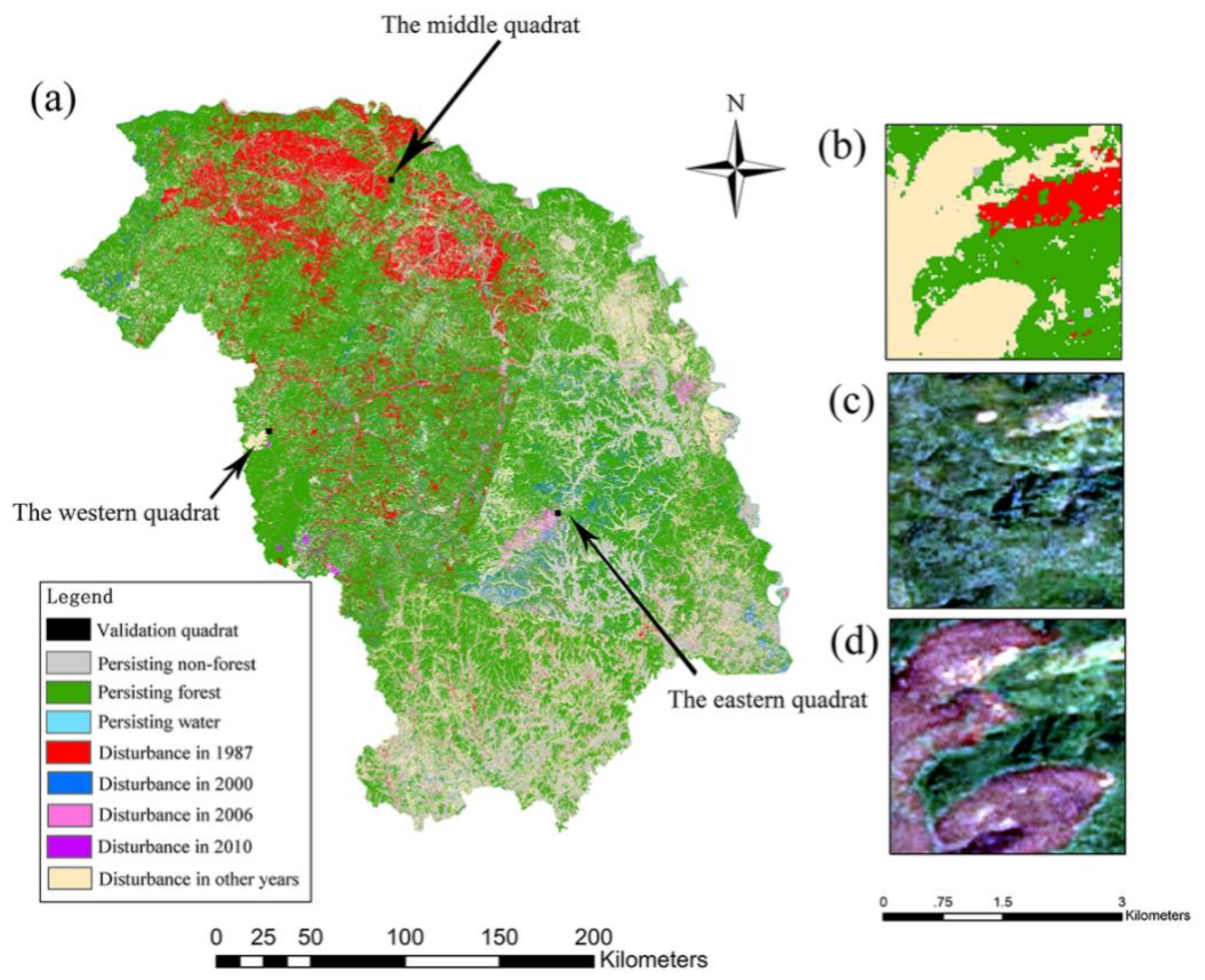
Additionally, we adopted the accuracy validation method proposed by Li et al. [34] to assess the accuracy of the forest disturbance maps using a spatial agreement index. Specifically, we used a spatial agreement index (SAI) based on visual interpretation and Google Earth high-resolution images to verify the accuracy of the VCT forest disturbance products. We randomly selected three 3 × 3 km squares in the study area as the validation area (Figure 2) to derive the SAI statistics using Equation (3).
S A I = S c d S g
In this method, S v is the disturbed area detected by VCT, S g is the disturbed area determined by visual interpretations, and S c d is the overlap area of the two detected regions. We superimposed the annual maps of aggregated forest and non-forest obtained from VCT in ArcGIS to obtain a map of the annual vegetation recovery status.

2.4. Burned Area Extraction Using the VCT Products and SVM Algorithm

We combined the SVM classifier and the disturbances detected by the VCT to extract the burned areas in 1987, 2000, 2006, and 2010. We used the SVM classifier because this algorithm has the advantages of seeking the best classification solution and dealing with a small number of samples [35]. Fires that occurred between 2012 and 2016 were excluded from the analysis because in the subsequent vegetation recovery modeling, we used the NDVI values of the fire patches in the fifth year after the fire to characterize the vegetation recovery status. Thus, the large fire events extracted in the current work included but were not limited to the “May 6th” fire in 1987, the Huma County fire in 2000, the Kandu River fire in the Songling area in 2006, and the Huzhong fire in 2010.
Several image features were extracted to conduct the SVM-based image classification to separate fire-affected areas from non-burned areas based on the Landsat time-series observations, including the original spectral bands, NDVI [36], Enhanced Vegetation Index (EVI) [37], Normalized Difference Moisture Index (NDMI) [38], Normalized Burn Ratio (NBR) [39], Normalized Burn Ratio 2 (NBR2) [40], and the Tasseled-Cap transformation (brightness, greenness, and wetness) [41].
N D V I = ρ N I R ρ R e d ρ N I R + ρ R e d
E V I = ρ N I R ρ R e d ρ N I R + 0.6 ρ R e d 7.5 ρ B l u e + 1.0
N D M I = ρ N I R ρ S W I R 1 ρ N I R + ρ S W I R 1
N B R = ρ N I R ρ S W I R 2 ρ N I R + ρ S W I R 1
N B R 2 = ρ S W I R 1 ρ S W I R 2 ρ S W I R 1 + ρ S W I R 1
where ρ N I R , ρ R e d , ρ B l u e   ,   ρ S W I R 1 , and ρ S W I R 2 are the surface reflectance in the Landsat TM/ETM+ bands 4, 3, 1, 5, and 7 and the Landsat OLI+ bands 5, 4, 2, 6, and 7.
We used the fire point data in 1987, 2000, 2006, and 2010 and the coordinates of the fire point data and grew burned pixels from the centers of 10–15 fire patches. The resulting number of burned pixels per year was around 500 (depending on the burned area in each year) (Table 1); these pixels acted as the training data for the burned area. Next, the non-burned pixels were identified from the false-color composites of the Landsat bands using visual interpretation, including forest, grassland, cropland, logging sites, built-up, and water. The number of non-burned pixels was nearly equal to that of the burned pixels. The identified pixels were then randomly divided into two groups; one group (70% of the pixels) was used for SVM classifier training, and the other group (30% of the pixels) was used for classification accuracy validation. In the SVM classification, the Gaussian radial basis function was regarded as the kernel function, the cost parameter C was 10 (representing a penalty for miss-classification errors), and γ was 50. Finally, a pixel was considered a fire disturbance pixel if it was labeled as a disturbance pixel by the VCT algorithm and was also classified as a burned pixel by the SVM. Thus, we were able to use fire points in each year of the Landsat time-series as training sets, and the SVM algorithm was used to extract the burned patches from the VCT-detected disturbances. As a result, the final dataset of forest fire patches in the four years was created by combining the VCT products and SVM algorithm. We used the remaining 30% of the pixels to create a confusion matrix to determine the overall accuracy, user’s accuracy, producer’s accuracy, and Kappa coefficient to quantify the reliability of the classifications.

2.5. Post-Fire Vegetation Recovery Modeling

In this study, we focused on fire disturbances that occurred in the Daxing’anling area. The NDVI is an efficient vegetation index in characterizing post-fire vegetation recovery [42]. Previous studies indicated that the NBR could be used to characterize recovery both in the short-term and long-term [43,44]; however, NDVI has the characteristics of rapid saturation and has been primarily used for shorter-term recovery assessments [45]. The increase in the post-disturbance NDVI value may be related to an increase in the cover of trees, shrubs, and herbaceous vegetation [30]. We focused on the early stages of post-fire vegetation recovery to reduce potential saturation effects. The NDVI value of the burned area in the first year was used as an independent variable to reflect the initial vegetation condition for possible vegetation recovery, whereas the NDVI values of the fifth year were used as the dependent variable to reflect the vegetative condition after recovery. Other independent variables included many topographic features (elevation, slope) [30], climatic factors (derived from meteorological station interpolation data) and fire severity (dNBR) (Table 2). Meteorological factors included the annual average temperature, precipitation, and moisture [46].
Three methods were selected to model post-fire vegetation recovery, including stepwise multiple linear regression (SMLR), SVM, and RF. Unlike the SMLR model, RF and SVM are non-parametric machine-learning algorithms that can deal with complex nonlinear relationships. RF has the advantages of determining variable importance, assessing the robustness of data reduction, high accuracy, and low sensitivity to parameter adjustments [47]. SVM is particularly well suited for a small sample size.
The SMLR was implemented by adding an important variable to or eliminating an unimportant variable from a collection of explanatory variables based on predetermined criteria. Typically, this step is performed using a series of F- or t-tests to evaluate the influence of a particular variable on the dependent variable [48]. This process was repeated twice until no new variables could be introduced into the model.
The RF algorithm has been widely used in data mining, ecology, and other disciplines [49]. An RF typically consists of a large number of regression trees, each of which has a set of constraints that are hierarchically organized and applied from the roots of the tree to the leaves. An RF starts with many randomly selected bootstrap samples that are iteratively replaced by those from the original training data set. Multiple regression trees are then generated to form an RF, and the final prediction result is obtained by averaging the predictions from all regression trees [50]. In the current analysis, we first defined two variable importance measures based on different response types before creating the RF. (1) After permutating each predictor variable randomly, the out-of-bag (OOB) error was used to compute the reduction in predictive performance. (2) The reduction in the node impurity can be quantified by the Gini index. Thus, the contribution of each predictor variable to the modeling performance was assessed and ranked. The percent increase in the mean square error (MSE) (PercentIncMSE) and the increase in the NodePurity (IncNodePurity) depend on the importance of the predictor variable. After multiple tries, we determined the following parameter values: The number of random regression trees (ntree) was 500, the number of segmentation variables (mtry) was 3, and the minimum sample size of the terminal node (node size) was 5.
The objective of the SVM is to minimize the prediction error and maximize the flatness of the function [51]. This trade-off is controlled by setting the error penalty factor C. The parameter ε is a zone defined around the regression function, and the error in the range of ±ε is ignored. If all the training tuples are in a zone with a width of 2ε, a function is output at the center of the flat channel containing all the training tuples, in which case the total error is 0. Therefore, ε controls the fitting degree between the function and the training tuples [52]. We used the same suite of independent variables derived from the stepwise regression analysis mentioned above in the SVM modeling and RF modeling to allow for the comparison of the models. A Gaussian kernel function was used; the error penalty factor C was 10, and ε-svr was the regression algorithm in the SVM regression.
We randomly selected around 100 pixels (the specific number depended on the recovery area) from the burned areas mapped by the VCT-SVM algorithm in each year and extracted the NDVI value and several impact factors for the 5 years (when the image was missing, we will use the image of next year) to fit the models. It is worth noting that collinearity usually exists among the meteorological variables. Thus, the selection of predictors used in the RF, SVM and SMLR models followed two steps: (1) we selected the predictors using the importance function in the RF model; (2) we eliminated the meteorological factors causing collinearity using SMLR [53]. An accuracy assessment was performed to assess the model’s prediction performance. In this study, we used 70% of the selected pixels for modeling and the remaining 30% for validation. We used the validation dataset to derive the mean absolute error ( M A E ), the coefficient of determination ( R 2 ), and the root mean square error ( R M S E ) to evaluate the prediction performance of the models.
M A E = 1 N i = 1 N y i y i ^
R 2 = 1 i = 1 N y i y i ^ 2 i = 1 N y i y i ¯ 2
R M S E = i = 1 N y i y i ^ 2 N
where y i is the observed NDVI value, y ^ i is the value predicted by the model, y ¯ is the average value of the observed samples, and N is the number of samples.

3. Results

3.1. Forest Disturbance Mapping and Validation

Table 3 shows the validation statistics derived from the three validation quadrats. It was observed that forest disturbances frequently occurred during the study period, and no disturbance was observed in seven, six, and four years in the study period in the eastern, middle, and western quadrat, respectively. Most of the spatial agreement ranged from 70% to 86%; the highest spatial agreement (92.35%) was observed in the eastern quadrat in 1987, and the lowest (60.03%) was observed in the western quadrat in 2010. Additionally, a very large disturbance patch was detected in 1987 (Figure 2); it was the site of “the May 6th” catastrophic fire in 1987 that led to 193 deaths, one million hectares of burned land (both inside and outside the study area), and 50,000 homeless people.
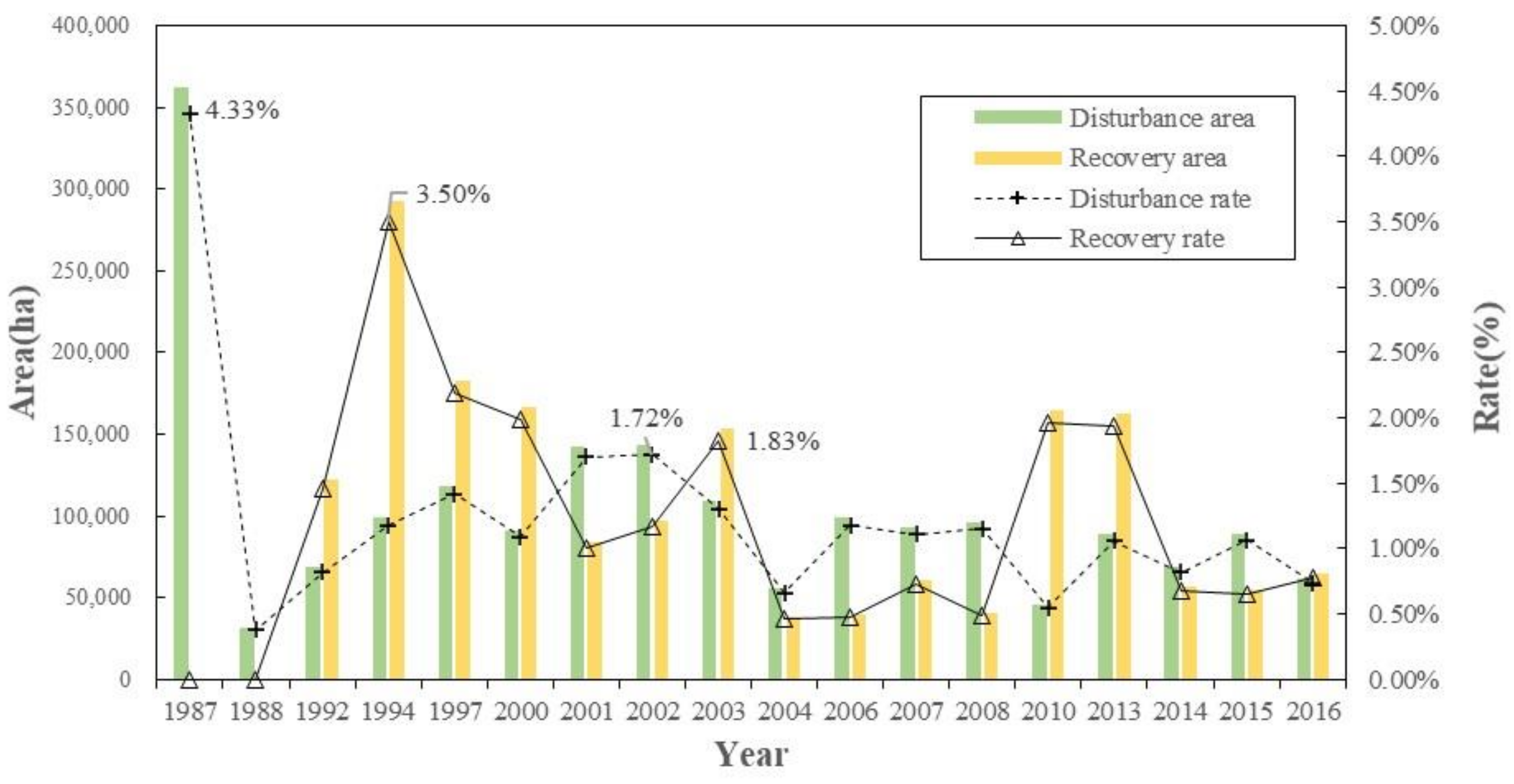
Figure 3 shows the dynamics of the disturbance and recovery events (disturbed forest area, disturbance rate, vegetation recovery area, and recovery rate) during 1987–2016 in the Daxing’anling region. The largest forest disturbance area was observed in 1987, with a total forest disturbance area of 362,288.8 ha and a disturbance rate of 4.33%; this result was primarily attributed to the 1987 “May 6th” catastrophic fire. The second- and third-largest disturbance areas occurred in 2001 and 2002, with similar areas of about 143,873 ha and similar disturbance rates of about 1.72%. The smallest disturbance area was observed in 1988, with an area of 31,708.98 ha and a disturbance rate of 0.38%. The largest recovery area was 293,112.5 ha in 1994, with a recovery rate of 3.5%, followed by 1997, with a recovery area of 182,858.5 ha and a recovery rate of 2.19%. The smallest recovery area was observed in 2004, with a recovery rate of 0.46%. Overall, except for these cases, the majority of the forest disturbance rates and recovery rates were less than 2%, and they fluctuated over time.

3.2. Fire Disturbance Mapping and Validation

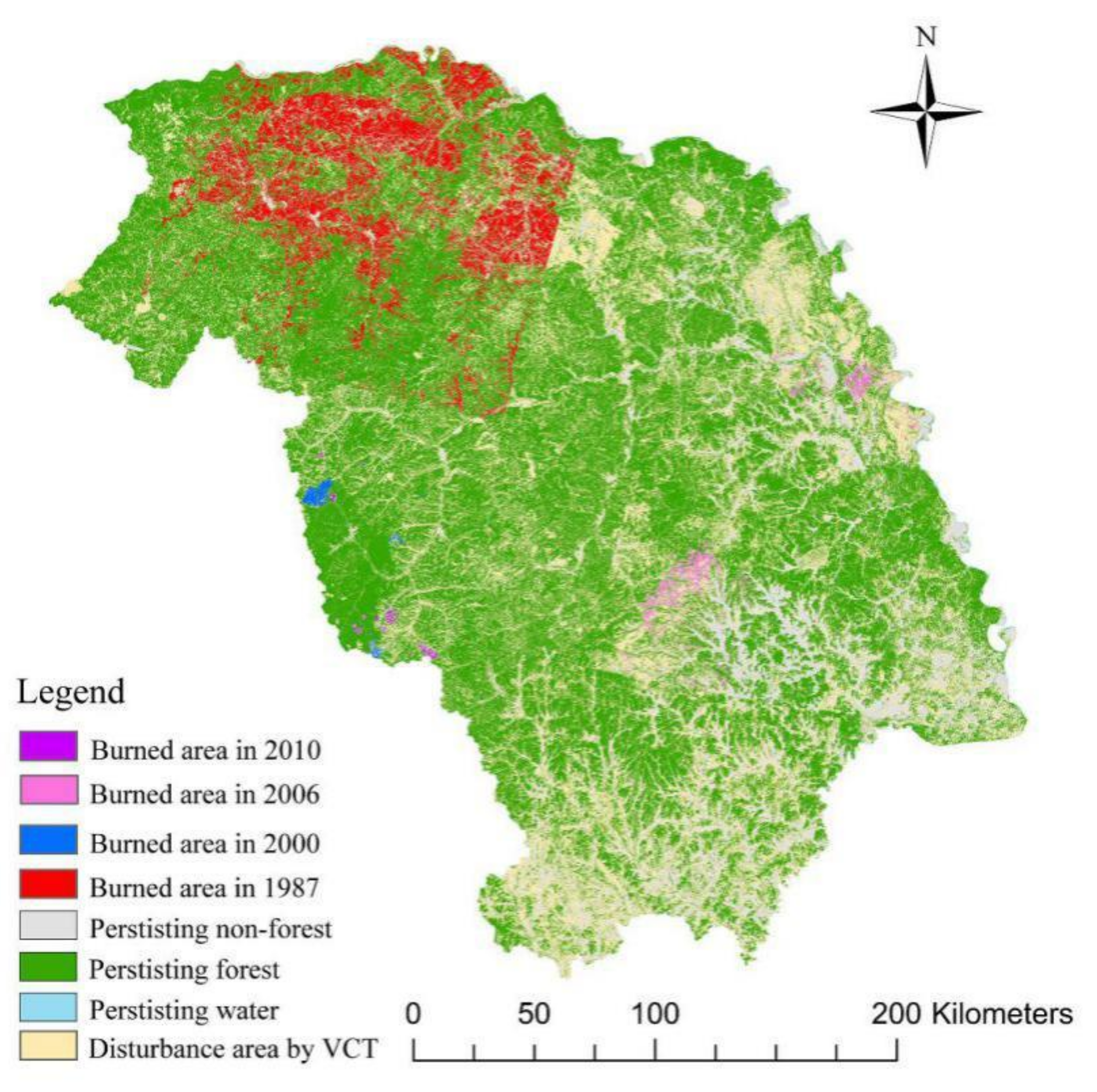
Figure 4 shows the spatial distribution of the burned areas extracted from the VCT-SVM algorithms, and Table 4 shows the error matrix derived from the independent samples. The classification accuracy of the fire patches was high, with an overall accuracy of 94% or higher for the four years. The user’s and producer’s accuracies were also above 90%, except for the 2016 producer’s accuracy (88.9%) of the non-burned class. The results show that Figure 4 is accurate and reliable, and the map can be used for the subsequent vegetation recovery analysis. Only two classes (burned area and non-burned area) were considered in the SVM classification. The burned areas were flagged as disturbance events by VCT, and small burnt areas (<1 ha) were excluded from the analysis. These strategies guaranteed the high extraction accuracy of the fire patches.

3.3. Model Fitting and Validation

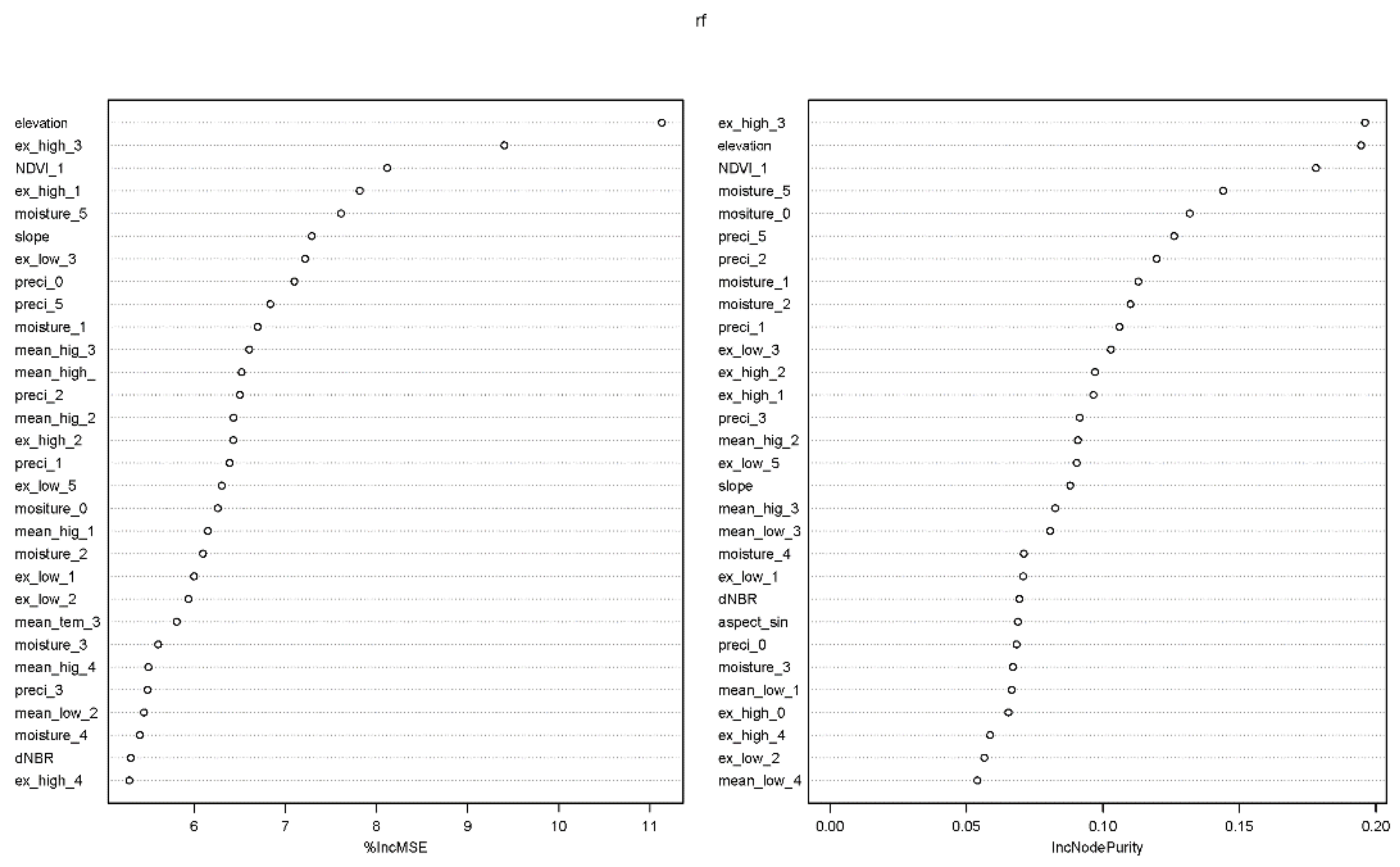
We first used the variable importance analysis in the RF package to identify the 25 most important potential environmental variables (Figure 5). Next, we implemented a stepwise regression analysis of the 25 potential variables to address the multicollinearity between the 25 variables to obtain the final set of 11 variables (Table 5).
The modeling results indicated that climatic factors played an important role in post-disturbance vegetation recovery of the first few years. The relative importance of the predictor variables (Figure 5) showed that the meteorological factors exhibited a good performance for vegetation recovery prediction. The precipitation factors in our study had high variable importance, indicating that precipitation was one of the limiting factors for vegetation recovery in this area. Although there was a good correlation between NDVI_5 and moisture_0, other moisture factors exhibited a poor performance for predicting the vegetation recovery status in this region. Extreme high temperatures, especially ex_high_3, performed well for vegetation recovery prediction.
Figure 6 shows the model fitting and validation results. RF outperformed SVM and SMLR regarding modeling performance. The R2 of the RF model fitting was 0.926, and the MAE and RMSE were lower than those of the SVM. The R2, MAE, and RMSE of the SVM fitting were 0.8288, 0.025, and 0.044, respectively. The results further showed that the validation R2 of the RF was higher than that of the SVM model (0.7113), with the highest validation R2 values of 0.7727.
The model evaluation results showed that the modeling accuracy and validation accuracy were higher for the RF than the SVM and SMLR (Figure 6). Overestimation of low values and underestimation of high values occurred in all three models, but these effects were least pronounced in the RF model.

4. Discussion

4.1. Fire Disturbance and Recovery

Since fire is a crucial factor resulting in forest decline in the Daxing’anling area [54], we assessed fire disturbance and recovery in this region using time-series analysis of remotely sensed spectral indices. The results were consistent with Zhang’s research describing a known burned forest area in the Daxing’anling area [55]. Our study identified a large disturbance event in 1987, which was consistent with the “May 6th” catastrophic fire in 1987. This was a catastrophic fire, leading to extensive loss of life and property and one million hectares of burned forest area (both inside and outside the study area) [56]. Post-fire recovery is affected by fire severity, biogeographic conditions, climate factors, forest management strategy, and other factors [30]. Thus, there are various recovery methods for different fires, including no land-use change, tree planting, or natural restoration; these practices have different effects on vegetation restoration [56]. Fire and post-fire recovery are crucial processes in sustainable forest management that shape the forest age, forest structure and forest type in northeastern China [30,57].

4.2. Post-Fire Recovery Response to Climate

The climatic factors had a substantial influence on post-fire vegetation recovery in this region, especially temperature factors play an important role in vegetation recovery in this region. Minore et al. pointed out that temperature was a critical factor for forest growth when sufficient moisture is available [58]. Extremely high temperatures (e.g., ex_high_3) and extremely low temperatures (e.g., ex_low_2) may limit post-fire vegetation recovery. Extreme temperatures might be a proxy for drought stress or indicate high solar radiation and temperature [30,59]. Precipitation factors were also important in this research, especially in the early stage (e.g., preci_1 and preci_2), which was in line with the findings by Meng et al. [30]. Liu also pointed out that higher growing-season precipitation one year after a fire had a positive influence on post-fire recovery [60]. Additionally, we found that topographic variables (especially elevation) in the modeling was important, which was supported by Bright [61]. However, this study selected the 5-year post-fire NDVI value as the post-fire state of recovery vegetation [22], and there may be a relationship between the elevation and the biomass amount [50], elevation was possibly less influential than our modeling results suggested. Lacking consideration of pre-disturbance state [22] can also explain the low importance of the dNBR, which was opposite to previous research [30]. Since the dNBR represents the difference in the NBR before and after the fire, the correlation between the dNBR and NDVI_5 (the amount of greenness at that time) was not high. However, fire creates favorable conditions for fire-adapted forest types to germinate and regenerate; therefore, some areas burned at higher severities and recovered more quickly than the areas at lower severities [31].

4.3. Vegetation Recovery Modeling

Although the overall performances of the three models are acceptable, the validation performances are inferior to the fitting performances, and overestimation for low values and underestimation for high values occurred in all three models (Figure 5). The reason may be that the fitting of the three models requires a large number of samples, and there were far more samples with intermediate values than with low values and high values, leading to inadequate or biased training of the model. In addition, the machine learning models, such as RF and SVM, performed better than SMLR. The likely reason is that most variables were non-normally distributed, causing visibly nonrandom trends in the residuals of the initial linear models [61].

4.4. Limitations and Future Improvements

Although important results were obtained in this study, the following aspects require further research: (1) Due to the limitations of VCT monitoring, ground-truth data, and the fire point data, some low-severity or small fires were not detected in the time-series data. Therefore, more sensitive spectral indices and more fixed-point field surveys are required in future research. (2) Vegetation indices are typically used for burned area extraction. However, some vegetation indices are highly correlated (such as NDVI and EVI), which may adversely affect the extraction result. (3) As mentioned above, we need to consider the pre-fire conditions to describe vegetation recovery. João used three indicators (compared with pre-fire condition) to measure different facets of the post-fire recovery process, which might be a better approach to capture recovery than NDVI_5 in our study [22]. (4) We used a small number of samples (3 quadrats) to verify the VCT disturbance results, which may have limited the ability to capture the heterogeneity and diversity of spatial, environmental, and spectral conditions in the area. Stratified random sampling will be considered to improve this problem [25]. (5) We did not consider the differences in forest type or tree species and only evaluated post-fire vegetation recovery of all forested areas. Different tree species may exhibit different recovery patterns after a fire and different responses to climate [30]. In future studies, different tree species and forest types will be considered to compare the post-fire recovery mechanism and provide comprehensive forest management suggestions after a fire.

5. Conclusions

Landsat time-series analysis can describe post-fire vegetation recovery at the landscape scale. In this study, a VCT-SVM method was used to extract fire disturbance areas and investigate vegetation recovery in burned areas. The RF, SVM, and SMLR models explained the relationship between post-fire vegetation recovery and different predictor variables, and the RF algorithm provided the best performance for predicting vegetation recovery after fire events. A good coupling relationship was observed between the climatic factors and post-fire vegetation recovery. The results of this study are applicable to other fire areas, where landscape-scale information on post-disturbance vegetation recovery is desired. The findings can inform management decisions and are suitable for carbon forecasting in forest ecosystems.

Author Contributions

Conceptualization, J.Q. and H.W.; methodology, H.W.; software, H.S., W.S., and Y.Z.; formal analysis, J.Q.; investigation, H.W.; data curation, J.Q.; writing—original draft preparation, H.W.; writing—review and editing, J.Q., Y.Z, M.L., and H.S.; funding acquisition, M.L. All authors have read and agreed to the published version of the manuscript.

Funding

This work was funded by the Natural Science Foundation of China, grant number 31971577. This research was jointly supported by the China Postdoctoral Science Foundation, grant number 2019M651842, and the Priority Academic Program Development of Jiangsu Higher Education Institutions (PAPD).

Data Availability Statement

Publicly available datasets were analyzed in this study. This data can be found here: [https://espa.cr.usgs.gov/, http://data.cma.cn/ (accessed on 24 December 2020)]. Fire point data was obtained from the Shenyang Institute of Applied Ecology at the Chinese Academy of Sciences and are available with the permission of the Shenyang Institute of Applied Ecology at the Chinese Academy of Sciences.

Acknowledgments

The authors would like to acknowledge the United States Geological Survey (USGS) and National Aeronautics and Space Administration (NASA) for providing the Landsat image data. Special thanks to the Shenyang Institute of Applied Ecology at the Chinese Academy of Sciences and the China Meteorological Data Network for sharing their fire data and climate data, respectively.

Conflicts of Interest

The authors declare no conflict of interest.

References

  1. Kelly, L.T.; Brotons, L. Using fire to promote biodiversity. Science 2017, 355, 1264–1265. [Google Scholar] [CrossRef] [PubMed]
  2. Westerling, A.L.; Hidalgo, H.G.; Cayan, D.R.; Swetnam, T.W. Warming and Earlier Spring Increase Western U.S. Forest Wildfire Activity. Science 2006, 313, 940–943. [Google Scholar] [CrossRef] [PubMed] [Green Version]
  3. Knorr, W.; Jiang, L.; Arneth, A. Climate, CO2 and human population impacts on global wildfire emissions. Biogeosciences 2016, 13, 267–282. [Google Scholar] [CrossRef] [Green Version]
  4. Sugihara, N.G.; Van Wagtendonk, J.W.; Shaffer, K.E.; Fites-Kaufman, J.; Thode, A.E. Fire in California’s Ecosystems; University of California Press: Oakland, CA, USA, 2006; p. 596. [Google Scholar]
  5. Chuvieco, E.; Mouillot, F.; van der Werf, G.R.; Miguel, J.S.; Tanase, M.; Koutsias, N.; García, M.; Yebra, M.; Padilla, M.; Gitas, I.; et al. Historical background and current developments for mapping burned area from satellite Earth observation. Remote. Sens. Environ. 2019, 225, 45–64. [Google Scholar] [CrossRef]
  6. Ramo, R.; Chuvieco, E. Developing a Random Forest Algorithm for MODIS Global Burned Area Classification. Remote. Sens. 2017, 9, 1193. [Google Scholar] [CrossRef] [Green Version]
  7. Chuvieco, E.; Martínez, S.; Román, M.V.; Hantson, S.; Pettinari, M.L. Integration of ecological and socio-economic factors to assess global vulnerability to wildfire. Glob. Ecol. Biogeogr. 2014, 23, 245–258. [Google Scholar] [CrossRef]
  8. Chen, J.M.; Zhao, P.; Guo, X.Y. Numerical simulation of the impact of changes in the vegetation in the western China on the summer climate over the northern China. Acta Meteorol. Sin. 2010, 68, 173–181. (In Chinese) [Google Scholar]
  9. Jeong, S.-J.; Ho, C.-H.; Park, T.-W.; Kim, J.; Levis, S. Impact of vegetation feedback on the temperature and its diurnal range over the Northern Hemisphere during summer in a 2 × CO2 climate. Clim. Dyn. 2011, 37, 821–833. [Google Scholar] [CrossRef] [Green Version]
  10. Jiang, B.; Liang, S. Improved vegetation greenness increases summer atmospheric water vapor over Northern China. J. Geophys. Res. Atmos. 2013, 118, 8129–8139. [Google Scholar] [CrossRef]
  11. Zou, Y.; Wang, Y.; Qian, Y.; Tian, H.; Yang, J.; Alvarado, E. Using CESM-RESFire to understand climate–fire–ecosystem interactions and the implications for decadal climate variability. Atmospheric Chem. Phys. Discuss. 2020, 20, 995–1020. [Google Scholar] [CrossRef] [Green Version]
  12. Furyaev, V.; Vaganov, E.; Tchebakova, N.; Valendik, E. Effects of Fire and Climate on Successions and Structural Changes in The Siberian Boreal Forest. Eurasian J. For. Res.-Hokkaido Univ. 2001, 2, 1–15. [Google Scholar]
  13. Arthur, A.D.; Catling, P.C.; Reid, A. Relative influence of habitat structure, species interactions and rainfall on the post-fire population dynamics of ground-dwelling vertebrates. Austral Ecol. 2012, 37, 958–970. [Google Scholar] [CrossRef]
  14. Gimeno-García, E.; Andreu, V.; Rubio, J.L. Influence of vegetation recovery on water erosion at short and medium-term after experimental fires in a Mediterranean shrubland. Catena 2007, 69, 150–160. [Google Scholar] [CrossRef] [Green Version]
  15. Gilroy, J.J.; Woodcock, P.; Edwards, F.A.; Wheeler, C.; Baptiste, B.L.G.; Uribe, C.A.M.; Haugaasen, T.; Edwards, D.P. Cheap carbon and biodiversity co-benefits from forest regeneration in a hotspot of endemism. Nat. Clim. Chang. 2014, 4, 503–507. [Google Scholar] [CrossRef]
  16. Shatford, J.P.A.; Hibbs, D.E.; Puettmann, K.J. Conifer regeneration after forest fire in the Klamath-Siskiyous: How much, how soon? J. For. 2007, 105, 139–146. [Google Scholar]
  17. Bassett, M.; Leonard, S.W.; Chia, E.K.; Clarke, M.F.; Bennett, A.F. Interacting effects of fire severity, time since fire and topography on vegetation structure after wildfire. For. Ecol. Manag. 2017, 396, 26–34. [Google Scholar] [CrossRef]
  18. Marlon, J.R.; Bartlein, P.J.; Daniau, A.-L.; Harrison, S.P.; Maezumi, S.Y.; Power, M.J.; Tinner, W.; Vanniére, B. Global biomass burning: A synthesis and review of Holocene paleofire records and their controls. Quat. Sci. Rev. 2013, 65, 5–25. [Google Scholar] [CrossRef]
  19. Lydersen, J.M.; North, M.P.; Collins, B.M. Severity of an uncharacteristically large wildfire, the Rim Fire, in forests with relatively restored frequent fire regimes. For. Ecol. Manag. 2014, 328, 326–334. [Google Scholar] [CrossRef] [Green Version]
  20. Mitri, G.; Gitas, I. Mapping Postfire Vegetation Recovery Using EO-1 Hyperion Imagery. IEEE Trans. Geosci. Remote. Sens. 2009, 48, 1613–1618. [Google Scholar] [CrossRef]
  21. Townshend, J.R.; Masek, J.G.; Huang, C.; Vermote, E.F.; Gao, F.; Channan, S.; Sexton, J.O.; Feng, M.; Narasimhan, R.; Kim, D.; et al. Global characterization and monitoring of forest cover using Landsat data: Opportunities and challenges. Int. J. Digit. Earth 2012, 5, 373–397. [Google Scholar] [CrossRef] [Green Version]
  22. João, T.; João, G.; Bruno, M.; João, H. Indicator-based assessment of post-fire recovery dynamics using satellite NDVI time-series. Ecol. Indic. 2018, 89, 199–212. [Google Scholar] [CrossRef]
  23. Shen, W.; Li, M.; Huang, C.; He, T.; Tao, X.; Wei, A. Local land surface temperature change induced by afforestation based on satellite observations in Guangdong plantation forests in China. Agric. For. Meteorol. 2019, 276, 107641. [Google Scholar] [CrossRef]
  24. Li, M.; Huang, C.; Zhu, Z.; Shi, H.; Lu, H.; Peng, S. Assessing rates of forest change and fragmentation in Alabama, USA, using the vegetation change tracker model. For. Ecol. Manag. 2009, 257, 1480–1488. [Google Scholar] [CrossRef]
  25. Zhao, F.; Huang, C.; Zhu, Z. Use of Vegetation Change Tracker and Support Vector Machine to Map Disturbance Types in Greater Yellowstone Ecosystems in a 1984–2010 Landsat Time Series. IEEE Geosci. Remote. Sens. Lett. 2015, 12, 1650–1654. [Google Scholar] [CrossRef]
  26. Tang, D.; Fan, H.; Yang, K.; Zhang, Y. Mapping forest disturbance across the China–Laos border using annual Landsat time series. Int. J. Remote. Sens. 2018, 40, 2895–2915. [Google Scholar] [CrossRef]
  27. Loboda, T.; Zhang, Z.; O’Neal, K.; Sun, G.; Csiszar, I.; Shugart, H.; Sherman, N. Reconstructing disturbance history using satellite-based assessment of the distribution of land cover in the Russian Far East. Remote. Sens. Environ. 2012, 118, 241–248. [Google Scholar] [CrossRef] [Green Version]
  28. Thomas, N.E.; Huang, C.; Goward, S.N.; Powell, S.; Rishmawi, K.; Schleeweis, K.; Hinds, A. Validation of North American Forest Disturbance dynamics derived from Landsat time series stacks. Remote. Sens. Environ. 2011, 115, 19–32. [Google Scholar] [CrossRef]
  29. Chu, T.; Guo, X. Remote Sensing Techniques in Monitoring Post-Fire Effects and Patterns of Forest Recovery in Boreal Forest Regions: A Review. Remote. Sens. 2013, 6, 470–520. [Google Scholar] [CrossRef] [Green Version]
  30. Meng, R.; Dennison, P.E.; Huang, C.; Moritz, M.A.; D’Antonio, C. Effects of fire severity and post-fire climate on short-term vegetation recovery of mixed-conifer and red fir forests in the Sierra Nevada Mountains of California. Remote Sens. Environ. 2015, 171, 311–325. [Google Scholar] [CrossRef]
  31. Meng, R.; Wu, J.; Zhao, F.; Cook, B.D.; Hanavan, R.P.; Serbin, S.P. Measuring short-term post-fire forest recovery across a burn severity gradient in a mixed pine-oak forest using multi-sensor remote sensing techniques. Remote. Sens. Environ. 2018, 210, 282–296. [Google Scholar] [CrossRef]
  32. Certini, G. Effects of fire on properties of forest soils: A review. Oecologia 2005, 143, 1–10. [Google Scholar] [CrossRef]
  33. Masek, J.; Vermote, E.; Saleous, N.; Wolfe, R.; Hall, F.; Huemmrich, K.; Gao, F.; Kutler, J.; Lim, T.-K. A Landsat Surface Reflectance Dataset for North America, 1990–2000. IEEE Geosci. Remote. Sens. Lett. 2006, 3, 68–72. [Google Scholar] [CrossRef]
  34. Li, M.; Huang, C.; Shen, W.; Ren, X.; Lv, Y.; Wang, J.; Zhu, Z. Characterizing long-term forest disturbance history and its drivers in the Ning-Zhen Mountains, Jiangsu Province of eastern China using yearly Landsat observations (1987–2011). J. For. Res. 2016, 27, 1329–1341. [Google Scholar] [CrossRef]
  35. Huang, C.; Song, K.; Kim, S.; Townshend, J.R.; Davis, P.; Masek, J.G.; Goward, S.N. Use of a dark object concept and support vector machines to automate forest cover change analysis. Remote. Sens. Environ. 2008, 112, 970–985. [Google Scholar] [CrossRef]
  36. Tucker, C.J. Red and photographic infrared linear combinations for monitoring vegetation. Remote. Sens. Environ. 1979, 8, 127–150. [Google Scholar] [CrossRef] [Green Version]
  37. Epting, J.; Verbyla, D. Landscape-level interactions of prefire vegetation, burn severity, and postfire vegetation over a 16-year period in interior Alaska. Can. J. For. Res. 2005, 35, 1367–1377. [Google Scholar] [CrossRef] [Green Version]
  38. Wilson, E.H.; Sader, S.A. Detection of forest harvest type using multiple dates of Landsat TM imagery. Remote Sens. Environ. 2002, 80, 385–396. [Google Scholar] [CrossRef]
  39. Wulder, M. Optical remote-sensing techniques for the assessment of forest inventory and biophysical parameters. Prog. Phys. Geogr. Earth Environ. 1998, 22, 449–476. [Google Scholar] [CrossRef]
  40. Stroppiana, D.; Bordogna, G.; Carrara, P.; Boschetti, M.; Brivio, P. A method for extracting burned areas from Landsat TM/ETM+ images by soft aggregation of multiple Spectral Indices and a region growing algorithm. ISPRS J. Photogramm. Remote. Sens. 2012, 69, 88–102. [Google Scholar] [CrossRef]
  41. Crist, E.P.; Cicone, R.C. A Physically-Based Transformation of Thematic Mapper Data-The TM Tasseled Cap. IEEE Trans. Geosci. Remote Sens. 1984, 22, 256–263. [Google Scholar] [CrossRef]
  42. Van Leeuwen, W.J.D.; Casady, G.M.; Neary, D.G.; Bautista, S.; Alloza, J.A.; Carmel, Y.; Wittenberg, L.; Malkinson, D.; Orr, B.J. Monitoring post-wildfire vegetation response with remotely sensed time-series data in Spain, USA and Israel. Int. J. Wildland Fire 2010, 19, 75–93. [Google Scholar] [CrossRef]
  43. Kennedy, R.E.; Yang, Z.; Cohen, W.B.; Pfaff, E.; Braaten, J.; Nelson, P. Spatial and temporal patterns of forest disturbance and regrowth within the area of the Northwest Forest Plan. Remote Sens. Environ. 2012, 122, 117–133. [Google Scholar] [CrossRef]
  44. White, J.C.; Wulder, M.A.; Hermosilla, T.; Coops, N.C.; Hobart, G.W. A nationwide annual characterization of 25 years of forest disturbance and recovery for Canada using Landsat time series. Remote. Sens. Environ. 2017, 194, 303–321. [Google Scholar] [CrossRef]
  45. Pickell, P.D.; Hermosilla, T.; Frazier, R.J.; Coops, N.C.; Wulder, M.A. Forest recovery trends derived from Landsat time series for North American boreal forests. Int. J. Remote. Sens. 2015, 37, 138–149. [Google Scholar] [CrossRef]
  46. Huang, C.; Goward, S.N.; Masek, J.G.; Thomas, N.; Zhu, Z.; Vogelmann, J.E. An automated approach for reconstructing recent forest disturbance history using dense Landsat time series stacks. Remote. Sens. Environ. 2010, 114, 183–198. [Google Scholar] [CrossRef]
  47. Breiman, L. Random forests. Mach. Learn. 2001, 45, 5–32. [Google Scholar] [CrossRef] [Green Version]
  48. García-Gutiérrez, J.; Martínez-Álvarez, F.; Troncoso, A.; Riquelme, J.C. A comparison of machine learning regression techniques for LiDAR-derived estimation of forest variables. Neurocomputing 2015, 167, 24–31. [Google Scholar] [CrossRef]
  49. Feng, Y.; Lu, D.; Chen, Q.; Keller, M.; Moran, E.; Dos-Santos, M.N.; Bolfe, E.L.; Batistella, M. Examining effective use of data sources and modeling algorithms for improving biomass estimation in a moist tropical forest of the Brazilian Amazon. Int. J. Digit. Earth 2017, 50, 1–21. [Google Scholar] [CrossRef]
  50. Shen, W.; Li, M.; Huang, C.; Wei, A. Quantifying Live Aboveground Biomass and Forest Disturbance of Mountainous Natural and Plantation Forests in Northern Guangdong, China, Based on Multi-Temporal Landsat, PALSAR and Field Plot Data. Remote. Sens. 2016, 8, 595. [Google Scholar] [CrossRef] [Green Version]
  51. Cao, X.; Chen, J.; Imura, H.; Higashi, O. A SVM-based method to extract urban areas from DMSP-OLS and SPOT VGT data. Remote. Sens. Environ. 2009, 113, 2205–2209. [Google Scholar] [CrossRef]
  52. Huang, C.; Davis, L.S.; Townshend, J.R.G. International Journal of Remote Sensing An assessment of support vector machines for land cover classification An assessment of support vector machines for land cover classi cation. Int. J. Remote Sens. 2002, 23, 725–749. [Google Scholar] [CrossRef]
  53. Hidalgo-Munoz, J.M.; Gamiz-Fortis, S.R.; Castro-Diez, Y.; Argueso, D.; Esteban-Parra, M.J. Long-range seasonal streamflow forecasting over the Iberian Peninsula using large-scale atmospheric and oceanic information. Water Resour. Res. 2015, 51, 3543–3567. [Google Scholar] [CrossRef] [Green Version]
  54. Yi, K.; Tani, H.; Zhang, J.; Guo, M.; Wang, X.; Zhong, G. Long-Term Satellite Detection of Post-Fire Vegetation Trends in Boreal Forests of China. Remote. Sens. 2013, 5, 6938–6957. [Google Scholar] [CrossRef] [Green Version]
  55. Zhang, Y. Study on the impacts of climate change on forest fires in Daxing’anling mountiains. Master’s Thesis, Northeast Forestry University, Harbin, China, 20 June 2008. (In Chinese). [Google Scholar]
  56. Chen, W.; Moriya, K.; Sakai, T.; Koyama, L.; Cao, C. Post-fire forest regeneration under different restoration treatments in the Greater Hinggan Mountain area of China. Ecol. Eng. 2014, 70, 304–311. [Google Scholar] [CrossRef] [Green Version]
  57. Cuevas-González, M.; Gerard, F.; Balzter, H.; Riaño, D. Analysing forest recovery after wildfire disturbance in boreal Siberia using remotely sensed vegetation indices. Glob. Chang. Biol. 2009, 15, 561–577. [Google Scholar] [CrossRef]
  58. Minore, D.; Laacke, R.J. Natural Regeneration; Oregon State University Press: Corvallis, OR, USA, 1992; pp. 258–283. [Google Scholar]
  59. Mildrexler, D.J.; Yang, Z.; Cohen, W.B.; Bell, D.M. A forest vulnerability index based on drought and high temperatures. Remote. Sens. Environ. 2016, 173, 314–325. [Google Scholar] [CrossRef] [Green Version]
  60. Liu, Z. Effects of climate and fire on short-term vegetation recovery in the boreal larch forests of Northeastern China. Sci. Rep. 2016, 6, 37572. [Google Scholar] [CrossRef] [Green Version]
  61. Bright, B.C.; Hudak, A.T.; Kennedy, R.E.; Braaten, J.D.; Khalyani, A.H. Examining post-fire vegetation recovery with Landsat time series analysis in three western North American forest types. Fire Ecol. 2019, 15, 8. [Google Scholar] [CrossRef] [Green Version]
Figure 1. Location of the study area in Northern China. The colored tiles on the right show the Landsat footprints (p119r024, p119r025, p120r023, p120r024, p120r025, p121r023, p121r022, p121r025, p122r023, p122r024, and p123r025), and the black polygon is the exact study site.
Remotesensing 13 00792 g001
Figure 2. (a) Forest disturbance patterns obtained from the VCT algorithm in the study area, including persisting forest, persisting non-forest, persisting water, and forest disturbance in different years; (b) annual forest disturbance patterns of the western quadrat; (c) Landsat image of the western quadrat before the disturbance in 1986; (d) Landsat image of the western quadrat after the disturbance in 2017.
Remotesensing 13 00792 g002
Figure 3. Annual forest disturbance and recovery areas and rates derived from the VCT products.
Remotesensing 13 00792 g003
Figure 4. Disturbance area obtained from VCT, persisting land cover types, and burned areas in the study region derived from the VCT-SVM algorithm.
Remotesensing 13 00792 g004
Figure 5. Variable importance ranking of all predictor variables. The acronyms of the predictive variable consist of two parts: abbreviation and number. Number means from the year after fire (the year of fire is 0) in the burned area. Abbreviation description: mean_tem (average annual temperature), ex_high (Extreme maximum temperature), ex_low (extreme minimum temperature), mean_high (average maximum temperature), mean_low (average lowest temperature), moisture (average relative humidity), preci (annual precipitation). A detailed description can be found in Table 2.).
Remotesensing 13 00792 g005
Figure 6. The fitting and validation results of the support vector machine (SVM), random forest (RF), and stepwise multiple linear regression (SMLR) (P < 0.01).
Remotesensing 13 00792 g006
Table 1. The number of burned/non-burned pixels in 1987, 2000, 2006, and 2010.
Year1987200020062010
Number of burned pixels429596311554
Number of non-burned pixels422611341557
Total85112076521111
Table 2. Description of the variables used in vegetation recovery modeling.
TypeVariableUnitDescription
Dependent variablePost-fire NDVI of the burned area in the fifth year (NDVI_5). Reflects vegetation restoration status after fire.
Disturbance effectPost-fire NDVI of the burned area in the first year (NDVI_1). Reflects site conditions (initial growth conditions and remaining trees).
dNBR dNBR = NBR pre NBR post
Reflects the fire disturbance severity.
Terrain factorsElevationMeterElevation
SlopeDegreeSlope
Aspect_cos Slope cosine
Aspect_sin Slope sine
Climate factorsmean_tem_0, mean_tem_1, mean_tem_2, mean_tem_3, mean_tem_4, mean_tem_5,Values*10Average annual temperature from the year of the fire (*_0) to the fifth year (*_5) after the fire in the burned area.
ex_high_0, ex_high_1, ex_high_2, ex_high_3, ex_high_4, ex_high_5Extreme maximum temperature from the year of the fire (*_0) to the fifth year (*_5).
ex_low_0, ex_low_1, ex_low_2, ex_low_3, ex_low_4, ex_low_5Extreme minimum temperature from the year of the fire (*_0) to the fifth year (*_5).
mean_high_0, mean_high_1, mean_high_2, mean_high_3, mean_high_4, mean_high_5Average maximum temperature from the year of the fire (*_0) to the fifth year (*_5) after the fire in the burned area.
mean_low_0, mean_low_1, mean_low_2, mean_low_3, mean_low_4, mean_low_5Average lowest temperature from the year of the fire (*_0) to the fifth year (*_5) after the fire in the burned area.
moisture_0, moisture_1, moisture_2, moisture_3, moisture_4, moisture_5Average relative humidity from the year of the fire (*_0) to the fifth year (*_5) after the fire in the burned area.
preci_0, preci_1, preci_2, preci_3, preci_4, preci_5 Annual precipitation from the year of the fire (*_0) to the fifth year (*_5) after the fire.
Table 3. The spatial agreements between the three randomly created validation plots (9 m2) and the forest disturbance map obtained from VCT.
Eastern QuadratMiddle QuadratWestern Quadrat
Disturbance YearSpatial
Agreement (%)
Disturbance YearSpatial Agreement (%)Disturbance YearSpatial
Agreement (%)
1987 72.351987 91.501987 78.15
1988 76.31 1988 74.34 1988No disturbance
1992 No disturbance1992 80.82 1992 69.31
1994 78.66 1994 No disturbance1994 61.01
1997 69.53 1997 70.00 1997 72.54
2000 62.31 2000 No disturbance2000 61.44
2001 No disturbance2001 75.93 2001 77.89
2002 89.53 2002 60.57 2002 89.63
2004 78.43 2004 No disturbance2004 No-disturbance
2006 66.16 2006 74.24 2006 74.92
2007 No disturbance2007 79.42 2007 70.08
2008 No-disturbance2008 73.91 2008 72.25
2010 66.82 2010No disturbance201060.03
2011 No disturbance2011 73.40 2011 71.30
201376.61 2013 73.93 2013 71.65
201471.52201478.34201470.81
2015No disturbance2015No disturbance2015No disturbance
2016No disturbance2016No disturbance2016No disturbance
Table 4. Error matrix for the classification of the burned areas in 1987, 2000, 2006, and 2010.
YearClassProducer’s AccuracyUser’s AccuracyOverall Classification AccuracyKappa Coefficient
1987Burned area100%93.9%95.2%0.905
Non-burned area90.3%100%
2000Burned area98.7%94.9%96.6%0.932
Non-burned area94.4%98.6%
2006Burned area98.7%90.3%93.9%0.877
Non-burned area88.9%98.5%
2010Burned area97.3%92.5%94.6%0.891
Non-burned area91.7%97.1%
Table 5. The variables selection results of the stepwise multiple linear regression (SMLR).
VariablesPearson Correlation Coefficient between the Selected Variables and NDVI_5EstimateStd. Errort-ValuePr(>|t|)
Intercept 2.36001415.76967820.4090.682871
NDVI_10.3930.29449530.07909363.7230.000244
mean_high_0 0.3000.17815340.03187285.596.08 × 10−8
mositure_0 0.350−0.44543230.0819126−5.4381.31 × 10−7
preci_1 0.3970.00043420.00020062.1640.031432
ex_low_2 0.2080.02890140.01032792.7980.005546
ex_high_3 0.3410.08793690.02315873.7970.000185
mean_low_3 0.198−0.09915070.0289456−3.4250.00072
preci_3 0.257−0.00026260.0001646−1.5950.111959
mean_high_4 0.197−0.12372210.0232963−5.3112.46 × 10−7
elevation 0.451−0.00020750.0001024−2.0270.043704
slope 0.261−0.0044640.0020547−2.1730.030774
Publisher’s Note: MDPI stays neutral with regard to jurisdictional claims in published maps and institutional affiliations.