Understanding Dense Time Series of Sentinel-1 Backscatter from Rice Fields: Case Study in a Province of the Mekong Delta, Vietnam

Abstract

Rice is the primary staple food of more than half of the world’s population and plays an especially important role in global economy, food security, water use, and climate change. The usefulness of Synthetic Aperture Radars (SAR) for rice mapping and monitoring has been demonstrated locally in many studies, in particular in the last five years with the availability of an unprecedented amount of free Sentinel-1 data within the Copernicus program. However, although earlier studies from the 1990s have laid the foundations of the physical understanding of the SAR response of rice fields, the more recent studies tend to overlook this aspect and to favor instead approaches driven by supervised learning which provide accurate results locally but cannot necessarily be extended to wide areas. The objective of this study is to analyze in detail the backscatter temporal variation of rice fields, using Sentinel-1 from 2015 to 2020 and in-situ data for the 5 rice seasons over 2 years 2017–2018, in order to derive robust SAR-based indicators useful for rice monitoring applications, which are essential for planning, monitoring and food security applications. The test region is the An Giang province, in the Mekong River Delta, Vietnam, one of the world’s major rice regions which presents a diversity in rice cultivation practices, in cropping density, and in crop calendar. The SAR data have been analyzed as a function of rice parameters, and the temporal and polarization behaviors of the radar backscatter of different rice varieties have been interpreted physically. New backscatter indicators for the detection of rice paddy area, the estimation of the sowing date, phenological stage and the mapping of the short cycle and long cycle rice varieties have been developed and discussed regarding the generality of the methods with respect to the rice cultural practices and the SAR data characteristics.

1. Introduction

Rice is the most important human food crop in the world and plays a special role in global economy, food security, and climate change—some of the most critical issues in the world [1]. For Asian developing countries where over 90% of the world’s rice is produced and consumed, rice agriculture is a key socioeconomic driving force [2]. However, with the extremely rapid growth of population, these countries face the challenge of attaining rice self-sufficiency to adequately feed the people [3]. Moreover, with the increasing effects of global climate change, extreme abiotic factors such as high temperatures, droughts, salinity, heavy rains, and floods are posing serious threats to rice production. In the context of threatened food security, comprehensive, reliable, and timely information on rice crop is highly needed at national to global levels. Moreover, rice agriculture is strongly linked to environmental issues including water consumption, and emission of greenhouse gases. Notably, inundated rice fields are one of the major generators of methane, accounting for 25% of the total budget of global methane emissions from agriculture [4]. For these reasons, global and long-term rice monitoring is also required.

The overall information which needs to be provided is the spatial distribution of rice fields, the status of rice growth for risk occurrence and annual production projections, together with the use of water resources and the related greenhouse gas emissions.

To this aim, remote sensing techniques are expected to provide synoptic information on spatial distribution of rice grown areas, along with rice growth status. Rice monitoring with remote sensing data has been demonstrated using a large variety of optical and microwave remote sensing data [5,6]. Because of the frequent cloud cover over major rice growing regions in particular in the tropics, Synthetic Aperture Radar (SAR) systems present the best alternative for rice crop monitoring for their all-weather capability and for the specific physical interaction between the radar waves and rice fields [7].

However, up to 2014, monitoring rice crop at national to continental scale was limited by the unavailability of cost-effective satellite SAR data with high temporal and spatial resolutions. With the launch of the first Sentinel satellite developed by the European Space Agency, providing a large and unprecedented amount of free data for the needs of the Copernicus program, operational use of SAR data for rice monitoring becomes possible. Sentinel-1A launched in April 2014, and Sentinel-1B, launched in April 2016 provide multi-temporal series of SAR imagery at C-band, at a time interval of 6 days. The available Sentinel-1 dense time series offer a unique opportunity to monitor rice crops in tropical regions, for long term programs, with the continuity of Sentinel data guaranteed up to 2030 and beyond.

Since the launch of Sentinel-1, a number of studies have been conducted to demonstrate the use of Sentinel-1 for rice crop mapping in many regions in Asia and Europe.

In these studies, the mapping methods can be grouped into two main categories.

• The first category uses supervised classification algorithms which require a large number of training samples of the same rice season. Machine learning techniques such as Random Forest or Support-Vector Machines have been used for rice mapping in India [8], in Myanmar [9], in Vietnam [10], in France [11], in China [12], and in Brazil [13]). More classical methods such as K-means have also been used, for example in India [14] and in China [15].
• The second category uses Rule-based detection algorithms based on knowledge of temporal signatures of rice fields in the study regions. This requires prior analysis of the backscatter of a number of monitored fields to derive feature descriptors, such as the modeled temporal curves, and the maximum, minimum, maximum increase of VV, VH, and VV/VH. Examples of such algorithms can be found in [16,17,18,19,20], and applications to Sentinel-1 can be found in [21,22,23,24,25,26].

Studies using the first category of methods have demonstrated that rice maps can be generated with good accuracy when (1) the rice cultivation is homogeneous in a region, in terms of crop calendar and cultural practices (i.e., transplanting vs. direct seedling, continuous flooding vs. intermittent drainage, rice cycle duration (short and long cycle varieties), and/or (2) the number of training samples is sufficient and representative for the diversity in rice cultivation. This requirement may be difficult to fulfill when dealing with large scale mapping for a region, a country, or a large part of a continent. For this reason, such approaches have been applied so far at local scales only.

In the studies using rule-based algorithms, some common features have been used, such as the high dynamic range of rice field backscatter with respect to other surface types, from the lowest backscatter at the start of season, to the highest backscatter at peak plant growth stage, in line with earlier observations and physical explanations [16].

Those methods exploit only first order statistics of the backscatter derived in the past from non-systematic data acquisitions. With Sentinel-1, dense (every 6 days or 12 days) data have been acquired systematically over most rice-growing areas in the world. The behavior of SAR time series over rice fields of a given region, if repeated from one year to another, can define backscatter temporal signatures which can be used to derive not only robust classifier of rice/non rice, but also information throughout the full rice cycle (estimation of sowing date and other phenological stages, estimation of rice cycle duration, etc.).

However, the multi-year backscatter temporal variation of Sentinel-1 data over rice fields has not been documented in detail, to assess how the temporal behavior of rice field backscatter change with rice varieties, varied management practices (e.g., tillage, transplantation, sowing, continuous vs intermittent flooding), and environmental conditions.

In order to develop robust methods based on the specific temporal signature of rice fields, it is essential to understand the temporal variation of the backscatter from rice fields and its underlying physical mechanisms. This will document the relevance and robustness of indicators used in rice mapping and monitoring of rice phenology, taking into account the diversity of rice crop and environment conditions. In most studies published since 2017 about the use of Sentinel-1 for rice monitoring, the physical interpretation that justifies the selected classifiers is either absent or speculative, partly because of the lack of complete and accurate in situ data to support the analysis of the SAR temporal profiles.

In this context, the objective of this study is to analyze the backscatter temporal variation of rice fields, using Sentinel-1 and in-situ data from 2015 to 2020, in order to support the development of robust rice monitoring methods coping with different rice cultivation systems encountered in a large region. The region under study is the An Giang province in the Vietnamese Mekong Delta, where the analysis has been carried out on 60 fields chosen to represent a diversity of conditions in rice varieties and management practices. The temporal backscatter curves are interpreted in terms of interaction mechanisms prevailing at different growth stages of the rice plants.

The paper is organized as follows: Section 2 will describe the test site and data used in this study, both the SAR data and ground data. Section 3 will present the analytical results, including a thorough analysis of the agronomic plant variables from the ground data, followed by the analysis of the temporal and polarization behavior of the radar backscatter of the rice fields and its physical interpretation in the light of the ground data. These results will lead to the discussion in Section 4 where SAR-based indicators for rice monitoring will be introduced and discussed. Section 5 will present the conclusions, with suggestions for future works.

2. Study Area and Data

2.1. Study Area

The study area is the Mekong River Delta (MRD), popularly known as the “Rice Bowl” of Vietnam, which covers an area of about 40,000 km² between 8.5–11.5° N and 104.5–106.8° E in the southern part of Vietnam. The MRD is the most important rice growing region, contributing up to 54% of total national rice production. The country’s important rice export sector is also centered here, with 90% of total milled rice exports originating from this region of Vietnam. A total of 12 provinces and 1 municipality constitute the Mekong Delta inhabited by about 17.4 million people, accounting for 20% of the population in the country. Geographically, the Mekong Delta is the last part of the Mekong River before it flows to the sea through a network of nine main distributaries. Vast areas of the MRD experience flooding on an annual basis, as a result of heavy monsoonal rainfall in the upper Mekong river catchment. The topography is very flat, with most of the land below 5 m. The climate of the Mekong Delta is monsoon tropical semi-equatorial with two well distinguishable seasons: the rainy season (June–November) and the dry season (December–May). Seasonal floods occur in a large part of the area, starting in August in the upper Delta, and then spreading to the lower Delta, peaking in September–October and lasting until the beginning of December. The floods bring large amounts of silt that contribute to the fertilization of the soil. The land is dedicated mostly to agriculture (63%), aquaculture (17.7%), and forestry (8.9%) (General Statistics Office of Vietnam) with the agricultural land comprising predominantly rice paddies (66% in area of annual crop), sugarcane, fruit tree plantation (particularly mango).

The MRD presents an important diversity of rice crop cultivation. The number of crops per year can vary from one to three (mostly three in the An Giang province), planted with short or long cycle rice, depending on the water management, including irrigation during the dry season and levee and dike construction to stop flood waters during the rainy season. The crop calendar can vary every year, depending on the onset of the rainy season, and because of the provincial regulations, the calendar can be specific to each of the 13 provinces. Rice farmers in the region have relatively small farms that are of 1 to 2 hectares on average and have mostly irrigated rice ecosystems with three major cropping seasons: Winter–Spring, Summer–Autumn, and Autumn–Winter cropping season.

Winter–Spring season or dry season rice where irrigation systems are available has the highest productivity (20.5% higher than the average yield of the region). Rice is planted at the end of the rainy season (November–December) and the increased solar radiation in the later cropping season from February–April provides good conditions during rice reproductive and ripening phases ensuring high productivity.

Summer-Autumn cropping season has the largest rice cultivation area, accounting for 54% of the total rice cultivation area of the region. Rice is planted in April–May before the onset of the rainy season. During the second part of the crop cycle and the rice is harvested in July–August before being devastated by floodwaters. Because of the lack of solar radiation, during the rainy period, the productivity is lower than for Winter Spring rice.

Autumn-Winter crop or rainy season rice crop has the lowest productivity. Rice is planted in July–August, and harvested in December–January. Rice area is the smallest in this rainy season, as almost 50% of the total area of the delta (4,000,000 ha) is flooded, in particular in the northern part of the delta due to the overflowing of the Mekong River in the upper reaches. However, in parts of the Delta, dike systems were built starting in the early 90′s in order to protect the fields from flood water to allow this third crop.

In a small part of the Delta not prone to floods, and without infrastructure for irrigation during the dry season, traditional rainfed rice still subsists. Rice is transplanted in July–August and harvested in November–December.

The water management varies across regions. A system of canals and dykes to bring irrigation water and to control floodwater has been built in the recent decades to complement the existing canal system that operated mainly as an irrigation source. In the rice fields surrounded by irrigation canals and dikes system, irrigation is performed using sluices and pumping apparatuses attached within the dikes of the paddies. Moreover, besides the traditional continuous flooding (CF) practice, modern water management has been developed in the last years, consisting in intermittent drainage between two irrigation operations, this is referred to as Alternate Wetting Drying (AWD). In both cases of water management, the rice fields are flooded before the date of sowing in order to prevent self-propagating vegetation and pests. At the end of the season, the fields are drained two weeks before rice harvest.

2.2. Ground Data

Ground data have been collected on sixty paddy fields for the Sentinel-1 time series analysis. Due to logistic reasons, the fields have been located in the province of An Giang, but were chosen to cover a range of rice planting practices, water management practices, rice varieties and crop calendar. The data have been collected regularly from April 2016 to April 2018, with a 3-month gap in the Summer–Autumn season in 2017 (from May to July). Among the parameters that impact the backscatter profiles of rice, as identified in the introduction, only the incidence angle has a restricted range of values in this dataset. With the available Sentinel-1 orbits, the An Giang province lies at an incidence angle range of around 43° ± 1° in descending orbit.

The ground data have been provided in GIS format for field delineation. To ensure low uncertainties in the mean radar backscatter over sampled fields, the size of most fields varies from 40 to 60 m in width and from 100 to 120 m in length. For 60 rice fields, ground data were collected at the dates of Sentinel-1 overpasses, every 12 days and 6–9 times per seasons as shown in Figure 1.

The general information, i.e., gathered once for each paddy field at each rice crop season, includes rice variety, planting method, seeding density, rice sowing and harvest dates and rice yield at harvest. The detailed ground data, i.e., collected at each visit in the field, comprise soil condition (1 for dry, 2 for wet, and 3 for water and mud), water layer thickness (cm), rice phenology, uniformity in plant height (1: yes; 2: no), plant height from the water or soil surface (cm). In all samples, photographs have been taken during the visits.

In terms of phenology, the following 12 growth stages scale have been used:

1: seedling, emergence	5: stem elongation	9. milky stage
2: 2/3 leaves	6: booting	10. milky-hard stage
3: tillering start	7. heading	11. maturing
4: tillering max	8. flowering	12. maturity

This scale was used by local experts and the Vietnam agriculture services for field survey to record the phenological stage.

2.3. SAR Data

Sentinel-1A and 1B data provide all-weather, day-and-night imagery at C-band (5.405 GHz) with an incidence angle roughly between 29 and 46°, operating in four exclusive imaging modes (Stripmap Mode, Interferometric Wide Swath Mode, Extra Wide Swath Mode, Wave Mode) with different spatial resolutions (down to 5 m) and coverage (with swath width up to 400 km). The platform follows a Sun-synchronous, near-polar, circular orbit at a height of 693 km. It provides dual polarisation capability (HH, VV, HH+HV, VV+VH), with revisit time of 12 days for one satellite, so that when the data are acquired by both satellites, data are available every 6 days, accessible rapidly, and free of charge [27].

This paper makes use of Sentinel-1 data acquired from October 2014 to March 2020. The data used are in Interferometric Wide Swath Mode (IW), having 2 polarizations VV, VH and a 250 km footprint in range direction, with 6-day acquisition interval for Sentinel-1A and 1B in descending mode. The Sentinel-1 images downloaded from the data hub are at the level 1-A (Level-1 Ground Range Detected (GRD)) products consisting of focused SAR data that has been detected, multi-looked, and projected to ground range using an Earth ellipsoid model (such as WGS84).

Figure 2 shows an example of one Sentinel-1 image covering the Mekong Delta.

The preprocessing was performed by the Sentinel-1 tiling processor: an automated chain developed by the French National Centre for Space Studies (CNES) and Center for the Study of the Biosphere from Space (CESBIO), based on the Orfeo ToolBox (OTB) utilities (https://www.orfeo-toolbox.org/ (accessed on 20 April 2019)) [28]. This processing chain handles the downloading of images from the Sentinel Product Exploitation Platform (PEPS) [29], followed by image preprocessing: calibration, orthorectification, and speckle filtering. After orthorectification, the equivalent number of looks (ENL) of pixel of 10 m is approximately 4.4. In order to increase this ENL, which is insufficient for most applications, we applied a multi-image filter which reduces the speckle effect while preserving the spatial resolution of the images [30,31]. A 3 × 3 spatial window was chosen and each image was filtered with the whole set of Sentinel-1 time series over each year.

3. Results

3.1. Ground Data Analysis

The data collected over 60 rice fields have been analyzed during 5 rice seasons in terms of rice crop calendar, rice variety, cycle duration, plant height, phenological stage, and water management.

Table 1. Summary of ground survey of 60 paddy fields under study over 5 rice cropping seasons.

Rice Seasons	IR 50404	Glutinous	Jasmine	Taiwan	OM 5451	Others	Total
Summer–Autumn 2016	32	5	2	11	4	6	60
Autumn–Winter 2016	34	4	4	11	3	4	60
Winter–Spring 2017	33	5	10	9	2	1	60
Autumn–Winter 2017	5	22	8	0	21	4	60
Winter–Spring 2018	25	26	7	0	0	2	60
Total	129 (43%)	62 (20.67%)	31 (10.3%)	31 (10.3%)	30 (10%)	17 (5.67%)	300
Rice–cycle variety	Short–cycle	Short–cycle	Long–cycle	Long–cycle	Short–cycle
Rice cycle duration (day)	85–100	90–103	97–110	100–120	90–100	85–100
Planting method	Direct seeding	Direct seeding	Transplanting	Transplanting	Direct seeding	Direct seeding
Seeding density (kg∙ha–1)	22–30	25–30	10–12	8–15	20–30

lists the number of surveyed fields for each of the main rice variety and each of the 5 rice cropping seasons, and for each variety, the planting method, seedling density, and the rice cycle duration. The repartition of the surveyed fields was done as much as possible to be close to that of the fields in the region: around 80% of short cycle varieties (<100 days) with direct seeding at high seeding density (>20 kg/ha) and 20% of long cycle varieties (>100 days) with transplantation and low density (<15 kg∙ha^–1). In all the surveyed fields, three crops of rice are grown in most years.

The characteristics of rice fields under study can be summarized as follows:

(1) Rice crop calendar:

Table 2. Sowing dates and harvest dates of the 60 paddy fields under study over five rice cropping seasons.

Rice Seasons	Sowing Period	Harvesting Period
Summer–Autumn 2016	29th March to 6th May 2016 (38 days)	29th June to 12th August 2016 (44 days)
Autumn–Winter 2016	5th August to 20th August 2016 (15 days)	1st November to 14th December 2016 (43 days)
Winter–Spring 2017	29th November to 26th December 2016 (27 days)	5th March to 15th April 2017 (41 days)
Autumn–Winter 2017	16th August to 10th September 2017 (25 days)	15th November to 20th December 2017 (35 days)
Winter–Spring 2018	15th December 2017 to 6th January 2018 (22 days)	18th March to 25th April 2018 (38 days)

shows the sowing period and the harvest period of 60 paddy fields over five rice cropping seasons. The sowing period of each rice season has been found expanded over 15 days (Autumn–Winter 2016), and up to 38 days (Summer–Autumn 2016). Meanwhile, the harvest dates of each rice season can differ between the paddy fields by up to 44 days (Summer–Autumn 2016). Overlapping among different fields has been found between the sowing period and the harvest period of two consecutive rice growing seasons, as can be seen in Table 2. However, despite the large span of sowing and harvest dates, at the administrative units (commune, district, provinces), the range of dates is relatively narrower, following local directives for agriculture management.

The calendar can be changed for the same rice season in different years, for example it was observed that the rice crop calendars of the rice seasons in 2017–2018 were delayed compared to the same rice season of in 2016–2017 (Table 2). Rice season of Autumn–Winter 2016 was started from 5th to 20th August 2016, and harvested from 1st November to 14th December 2016, while Autumn–Winter 2017 rice season was started from 16th August to 10th September 2017 and harvested from 15th November to 20th December 2017, about more than 10 days later than the previous year calendar. Similarly, the sowing dates of Winter–Spring 2018 (from 15th December 2017 to 6th January 2018) were found later than the sowing dates of Winter–Spring 2017 (from 29th November to 26th December 2016). It is also observed that the fallow time between two consecutive rice seasons is spanned from a week up to 45 days, depending on the rice variety and the crop season. The recuperation period between Summer–Autumn and Autumn–Winter is observed to be shorter than the one after Autumn-Winter season, due to the floods that occur (from October to December).

(2) Rice varieties and cycle duration: The dominant varieties in surveyed rice fields were short-cycle rice varieties including IR 50404 (43%), Glutinous (20,67%), and OM5451 (10%), and long-cycle rice varieties account for 20.6% (Jasmine and Taiwan) in line with the rough estimate of the percentage of the long and short cycle rice in the region.

The short-grain rice varieties such as IR 50404 or OM5451 have short cycle duration from 85 to 100 days. The long-grain, long growth cycle varieties (Taiwan and Jasmine) have cycle durations from 100 to 120 days. As a consequence, long rice cycle variety has a much shorter recuperation period (about 7–10 days) compared to short cycle rice. The long and short cycle rice fields differ in planting practices: direct sowing for short cycle rice and transplantation for long cycle rice. For transplantation, the seedlings are prepared and then transplanted to the inundated fields to provide regular spacing between the plants, with a seeding density of 10–15 kg∙ha^–1. For the direct sowing, the seeds are thrown to the wet fields by hand or machine with the variable seeding density from 20 to 30 kg∙ha^–1. It can be seen that transplanting crop saved more than 50% of the seeds. 80% of farmers were using the direct seeding in order to eliminate the laborious process of planting seedlings by hand and greatly reduce the land preparation time and the crop’s water requirements. However, the market price is much higher for long-cycle rice, because of the rice grain quality [32]. As a consequence, the long-cycle rice, long time abandoned, is more and more recovered in the region [20].

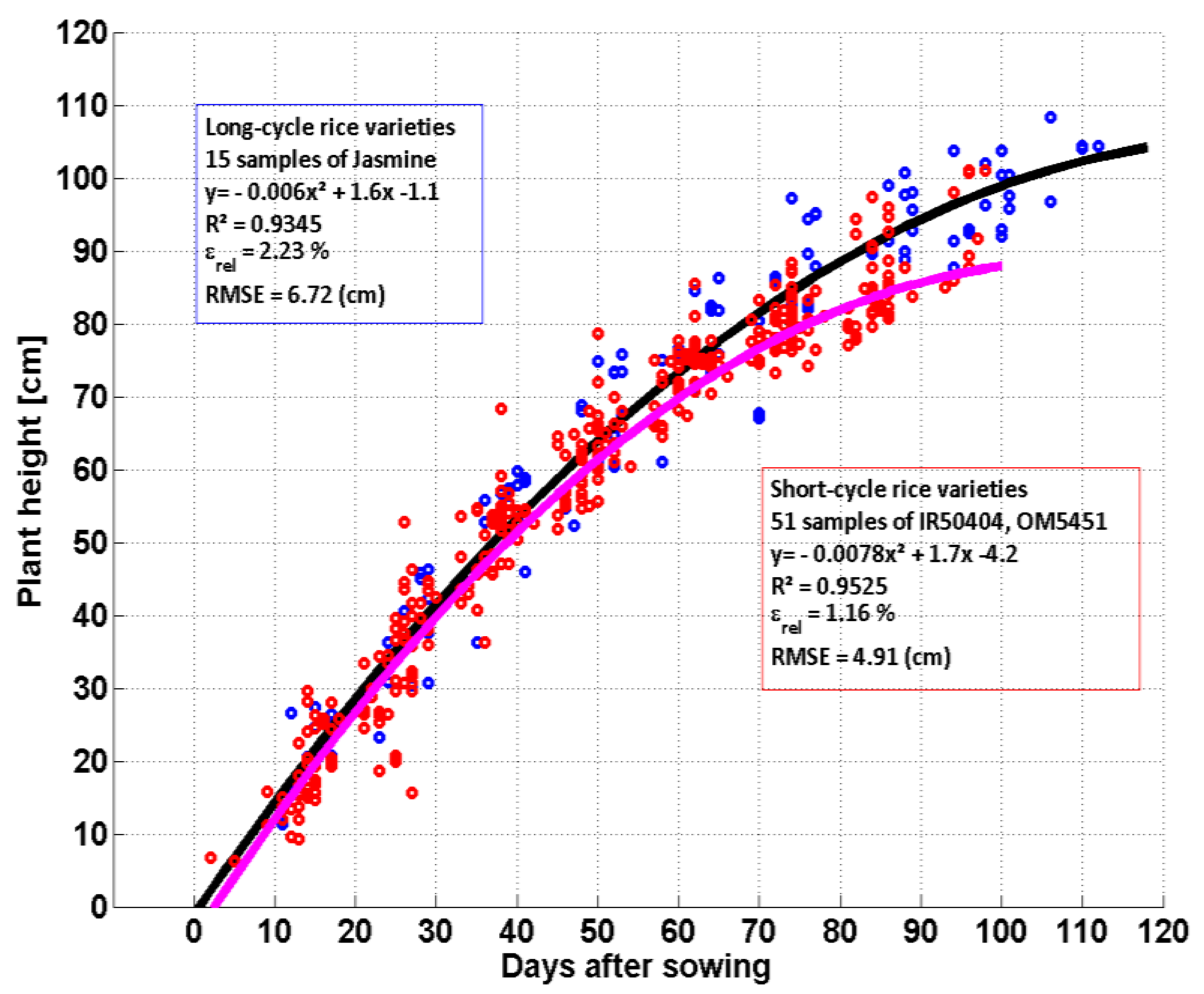
(3) Plant height, phenological stage and water management:Figure 3 shows the temporal variation of the plant height as a function of plant age (days after sowing). The analysis is applied separately to long cycle rice fields (15 fields of Jasmine) and short-cycle rice fields (51 fields of IR50404, OM5451). The same increasing trend is observed until 50–60 days when the plants reach 60–75 cm for both groups. This trend has been observed in previous studies on monitoring paddy rice fields [11,20].

From 60 days after sowing (beginning of reproductive phase for short cycle rice), the short cycle rice variety shows a smaller increase rate until 95 days, while long cycle rice variety continues at the same rate until 110 days. Two empirical polynomial regression curves of plant height have been derived. A coefficient of determination R² = 0.93 and a RMSE of 6.72 cm was obtained for long cycle variety group and R² = 0.95 and a RMSE of 4.91 cm for short cycle variety group Figure 3.

Figure 4 shows the phenological stage, from 1 to 12, as a function of days after sowing (DAS). The distribution of surveyed data at each stage is represented by a box-and-whisker plot based on five representative quantities: minimum, first quartile, median, third quartile, and maximum. Outliers are also singled out. This analysis also makes use of two groups of short cycle rice (51 fields) and long cycle rice (15 fields). The growth stages of short and long-cycle rice follow the same trend until stage 6 (booting-50 days after sowing). From stage 7 (heading, 60 days after sowing) onwards, short cycle rice grows reaching the following stage every 3–5 days while long cycle rice continues to grow reaching the next stage every 7–10 days. This observation is consistent with the trend in plant height, similar up to 50 days, then divergent after 60 days (Figure 3).

(4) The different phase of the rice cycle, together with cultural practices and plant and canopy description: Based on the ground data and on the field survey, the different phases in the rice growth cycle in the region under study can be summarized below. Figure 5 shows photographs which illustrate some of the phases:

For short cycle rice:

• 1–2 weeks before sowing, the fields were flooded in order to prevent self-propagating vegetation and pests. 1–2 days before sowing, the fields were drained (Figure 5a). Rice seeds were directly sown on wet soil by drilling (precision equipment) or broadcasting (hand). 3–4 days after sowing, the fields were irrigated (2–3 cm) just for 1 day then drained to ensure sufficient soil moisture to facilitate seed germination.
• 10–15 days after sowing (stage 2, plant height at about 15–20 cm, 2–3 leaves). The fields were inundated during this period for the roots to grow smoothly.
• 15–25 days after sowing (stage 3, plant height at about 20–35 cm, beginning of tillering). During the tillering period, the rice grows rapidly and strongly in roots and leaves. This period is the key in the development of the number of leaves, leaf area and number of effective tillers (for the number of future panicles). The duration of the tillering phase depends on the variety, cultivation methods and environmental conditions. In favorable solar radiation and nutritional conditions, this period lasts about 20–25 days. The fields were irrigated 2–3 times for about 5–10 cm of water layer and water kept for 2–3 days each time. It is important to note that about 20 days after sowing, the rice plant loses its vertical structure.
• 25–35 days after sowing (stage 4, the plant height is at about 35–45 cm, and the plant reaches the end of tillering). Farmers keep only 3–5 effective tillers per plant and eliminate the others to optimize the nutrition consumption as well as avoiding pest infestation. The fields were irrigated during fertilizing for a couple of days then drained to kill pest. Alternate wet/dry irrigation (AWD) was applied (mostly in the dry season) from this stage to save irrigation water.
• 35–45 days after sowing (stage 5, stem elongation, plant height is at about 45–58 cm, and the plant reaches stem elongation). Plant is growing straight up and denser.
• 45–58 days after sowing (stage 6, the plant height is at about 58–70 cm, the plant is at booting stage). The first step is the process of differentiation and formation of reproductive organs, and this process directly affects the rice yield. During this period, rice has significant changes in morphology, leaf color, physiology, and resistance to external circumstances. The initial panicle has been formed and prepared for heading. From the panicle initiation stage, three more leaves have been formed. Until this stage, the rice plants finish the vegetative phase (tillering, elongation, and booting) which is characterized by an increase of the plant height, an increase of the number of tillers, and a development of leaves.
• 58–65 days after sowing (stage 7, heading). When the booting period is finished, the heading starts the reproductive phase. The entire panicles are heading from the leaf sheath. The process is finished within 4–6 days.
• 65–75 days after sowing (stage 8, plant height at about 70–80 cm, flowering). It takes about a week for the flowers on the same panicle to blossom. After 10 days, all the flowers are fertilized and begin to develop into seeds.

During the reproductive phase (heading, flowering) the plant is characterized by a decrease of the number of tillers, the development of panicle leaf, the panicles formation and development. After heading (i.e., around 60 days after sowing), the growth (height, plant biomass) stops and the leaves change their orientation, to be no more erectophile (Figure 5d).

• 75–85 days after sowing (stages 9, 10, milky stage). The biomass of grains strongly increases during this period, reaching 70–80% of the final grain biomass. The heavy panicle curls down.
• 85–100 days after sowing (stage 11, 12): maturity stage.

During the ripening phase (grain filling, milk, and maturity), a decrease of leaf and stem moisture content and a decrease of the number of leaves are observed. The irrigation is stopped during the latter part of this period until harvest.

For long cycle rice, the vegetative phase development was similar to the short rice cycle until stage 6. From stage 7 onwards, rice develops with 4–5 days longer at each stage compared to short rice cycle to end its cycle duration of 110–120 days.

The analysis shows that during the rice cycle development, the plant structure changes at key phenological stages (Figure 5c,d). This can be used to understand and interpret the temporal and polarization behavior of the radar backscatter. In particular, the structure changes at the beginning of tillering, and the booting-heading (about 20 days and 60 days after sowing), independently of the rice variety, can lead to the development of backscatter indicators for rice phenological stages.

3.2. Sentinel-1 Time Series Analysis and Physical Interpretation

This section will analyze and interpret the temporal variations of Sentinel-1 backscatter in terms of interaction mechanisms prevailing at different polarizations, and over different growth stages of the rice plants. This will allow assessing the impacts of cultural practices on the backscatter time series.

3.2.1. Seasonal Variation with Regard to the Phenological Stages

In order to understand the seasonal variation of the backscatter with regard to the phenological stages of rice plant and field condition, we show in Figure 6b the backscatter time series of VH, VV, and the VH/VV ratio in the Autumn–Winter 2017 rice season.

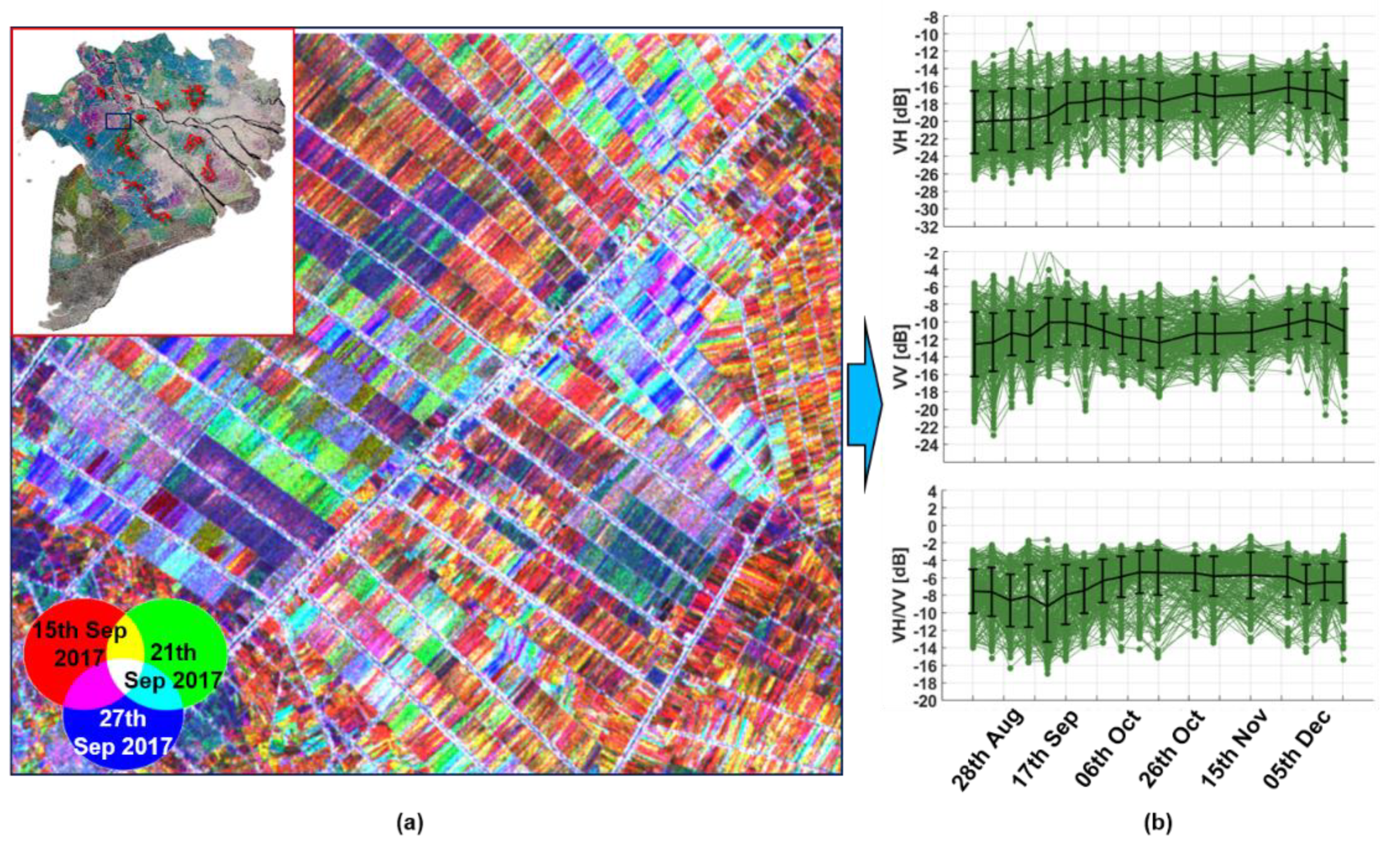
In Figure 6b, these time series are plotted as a function of the acquisition date for 200 fields: the 60 fields from the An Giang province reference dataset, complemented with 140 fields situated in eight surrounding provinces and identified using high-resolution optical data from Google Earth. At a given date, the backscatter variability is very large, notably at the beginning of the season: for example, at the second Sentinel-1 (referred to as Sentinel-1 hereafter) date, the inter-field dynamic range of VH and VV are respectively around 15 dB and 17 dB, and the standard deviation around 4 dB; whereas the smallest range, found at the beginning of November, is about 10–12 dB with a 2 dB standard deviation. This large variability is explained mostly by the fact that the planting calendar may be different between provinces, and between communes, districts within a province. Moreover, the fields may have different rice varieties, planting practices and management. This is exemplified in Figure 6a which shows a color composite of VH at three consecutive dates (15th, 21st, 27th September 2017) over rice fields in the region, where the rice fields appear in different colors. These different colors represent different backscatter value combinations for the 3 dates. For example, areas in green correspond to pixels with a higher backscatter in the green channel (21st September 2017) than in the red and blue channels (15th and 27th September 2017). Different colors in the RGB composite indicate different crop conditions (irrigation soil, phenological stages...).

This inter-field variability makes it difficult to use supervised approaches to classify rice pixels at a given Sentinel-1 acquisition date, as it would require the collection of a very large number of reference samples, for different groups of rice fields, with the procedure to be repeated at each season. The averaged curves in Figure 6b show that the temporal variation is different between VH and VV, with an overall dynamic range of 2 to 3 dB.

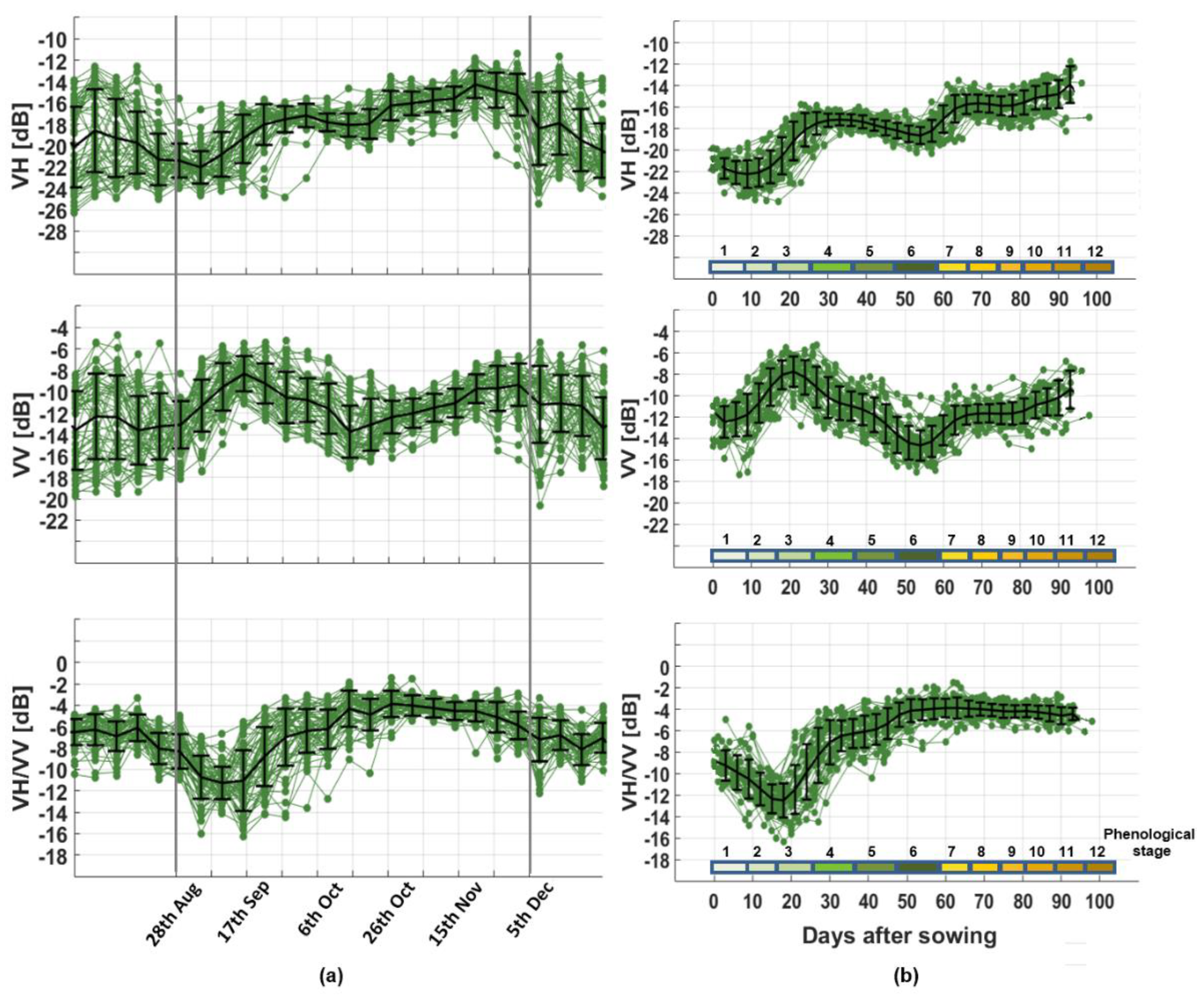
In order to analyze the temporal profiles in more details, Figure 7ashows the backscatter profiles plotted as a function of the acquisition date for the 60 reference fields only, which are located in the same province. The inter-field variability is found significantly reduced, with the smallest range at the beginning of November of about 4–5 dB and standard deviation of 1 dB for VH and VV. The variability is large at the beginning of the season, 11 dB and 13 dB, with 2–3 dB standard deviation, for VH and VV, is explained by the fact that, at the beginning of the season, the fields have a diversity of status, from bare fields, flooded or not, to rice plants at early and late growth stages.

Finally, the inter-field variability is found further reduced by plotting in Figure 7b the temporal variations as a function of the number of days after sowing (DAS), instead of the acquisition date. The inter-field dynamic range decreases to about 4-6 dB, with standard deviation of 1–2 dB indicating a specific temporal behavior of the 60 rice fields.

We provide here a physical interpretation of this backscatter temporal behavior, based on the information from the ground data.

At the early stage (0–20 days, stages 1 to 3, leaf emergence): The radar backscatter values at VH and VV polarizations are that of wet soil surface at the sowing date (−11 dB for VV and −21 dB for VH). About 10 days after sowing, the fields are flooded, leading to low backscatter of water surface at that date (−13 dB for VV and −22 dB for VH). A small decrease of backscatter is observed at 10 days. The water layer remains during few days (10–15 days after sowing). From 10 to 20 days after sowing, with the vegetation growth, VV increases steadily of 5–6 dB and VV reaches its maximum at 20 days after sowing, whereas VH increases of 2–3 dB and continue to increase after this day. The increase is interpreted as due to volume scattering (i.e., scattering from the vegetation), and double bounce scattering (i.e., wave interaction between vegetation and the ground: water layer or wet soil) [16], the latter being more important at VV than at VH. Because of the higher backscatter and strong increase of VV, the VH/VV ratio keeps on decreasing from the day of sowing to reach the minimum value at tillering stage at around 20 days.

From about 20 to 55 days (stages 3 to 6, tillering to booting), the plant is characterized by an increase in the plant height (from 30 to 70 cm), an increase in the number of tillers, and the full development of leaves, and by a vertical plant structure (Figure 5d). The rice canopy becomes denser, leading to an increasing attenuation in volume backscatter, and in a lesser extent, in double bounce scattering. At VV, the attenuation is enhanced by the vertical structure of the plant, causing a very strong decrease, up to 10 dB in about 1 month. At the same time VH increases until about 25 days then remains stable or slightly decrease due to attenuation until about 55 days but much less drastically (3–4 dB). As a consequence, the VH/VV ratio increases first at a higher rate during tillering (about 7 dB in 10 days), then at a moderate rate (3–4 dB in 20 days) before booting. The increase in VH/VV can be therefore interpreted as the differential attenuation in VH and VV. The contribution from the ground surface, mainly through the double bounce term, present in both VH and VV [33], is expected to be less important in non-flooded than flooded rice fields (specular reflection in flooded fields vs. scattering in non-flooded soil) and less important in denser canopy because of the higher attenuation of the wave by the vegetation. In addition, this contribution is minimized in the ratio. The backscatter ratio, having reduced contribution from ground scattering, should have a higher correlation with the plant’s parameters such as biomass or Leaf Area Index (LAI), as reported by studies [34] for other cereal crops.

From 55 to 65 days (stage 6 to 7, booting to heading), the plant is characterized by an erectophile structure, leading to attenuation in VV and VH. At 60 days, both VV and VH reach a minimum in the backscatter. Following this stage, the development of panicle leaf, the panicles formation, and the increases in biomass, contribute to an increase of the volume scattering in VH and VV. The radar backscatter therefore increases at both VH and VV polarizations (4–5 dB in a week). The VH/VV ratio remains stable until the end of its cycle.

From 65 days to maturing stage (stages 8–12), the leaves and stem biomass decreases, and the grain biomass increases to reach 70–80% of the final values, a small increase (2–3 dB) is observed for both VV and VH, and a small decrease (<1 dB) in VH/VV.

One notable finding of this analysis is the peculiar temporal behavior of the VV backscatter during the rice season compared to what was observed in past studies. Most studies have reported that the C-band backscatter of rice fields at VV polarization is globally characterized by a marked increase from sowing/transplanting to heading, followed by a plateau or a slight decrease during maturation. This was observed not only from satellite SAR sensors such as the European Remote-Sensing (ERS) or the Advanced Synthetic Aperture Radar (ASAR) [16], but also through electromagnetic modelling [35] and in-field scatterometer measurements [36]. Likewise, the recent observations with Sentinel-1, indicated a similar behavior in several studies [23,37,38]. This discrepancy can be explained by several factors. First, the cultural practices (sowing vs. transplanting, high vs. low plant number density, permanent flooding vs. intermittent drainage) change between regions and epochs. This has an impact on the backscatter through the physical interaction mechanisms: the waves attenuation is stronger for higher plant number density, the contribution of the ground scattering and the double bounce plant-ground scattering in the overall backscatter are reduced when the canopy is denser, and when the ground is not inundated. Second, the higher observation frequency of Sentinel-1 (every 6 to 12 days) allows more detailed observations compared to previous sensors (35 days for ERS or ASAR). Regarding VH, previous studies did not report the slight backscatter decrease that is observed with Sentinel-1 in the Mekong delta between tillering and booting [36,39].

3.2.2. Inter-Season Stability

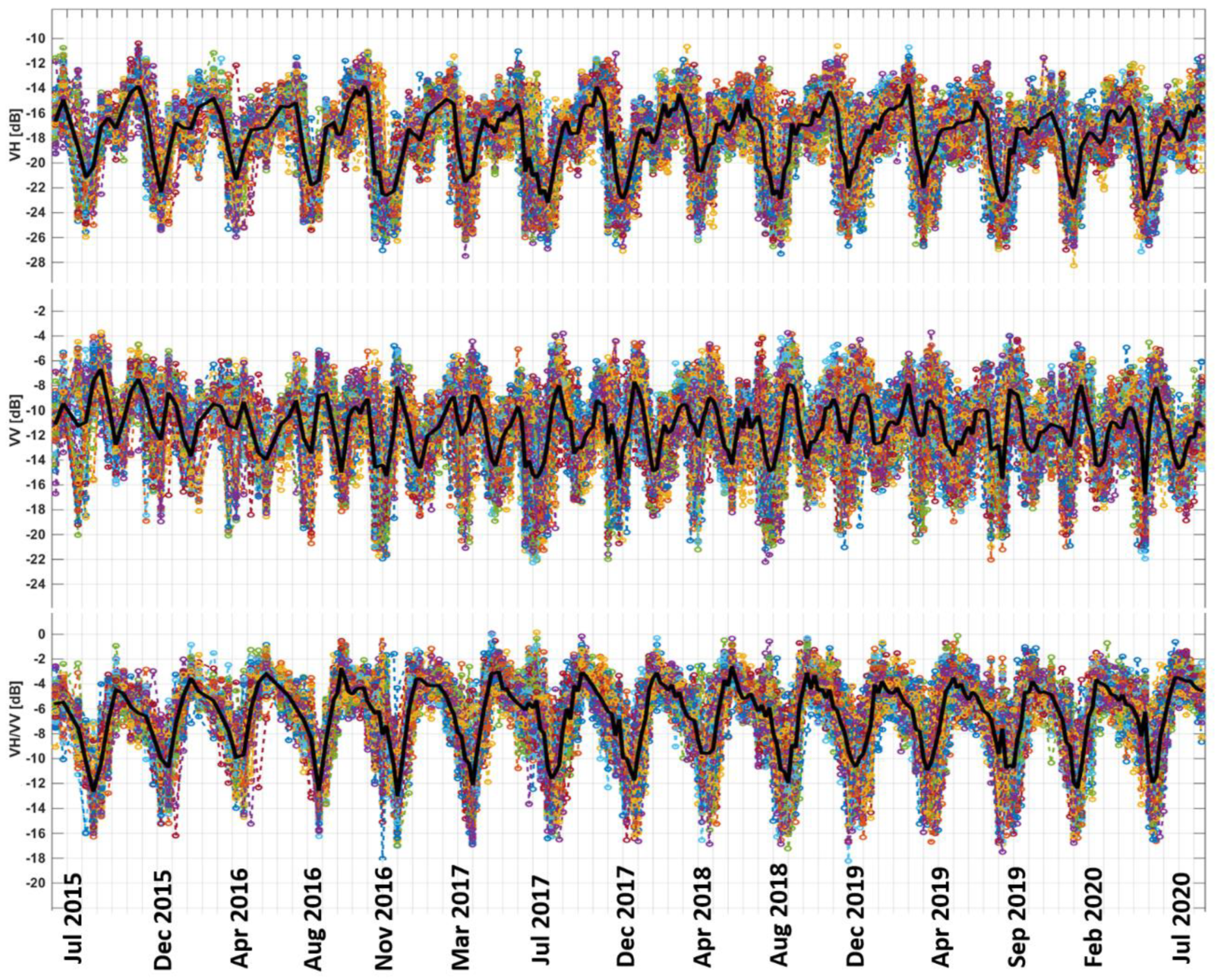
As this backscatter behavior of the rice fields observed in the 2017 Autumn–Winter season differs significantly from previously reported observations, we wanted to check that it represents an actual pattern in the Mekong Delta, and that is not an observation caused by exceptional conditions. To do so, we have plotted in Figure 8 the backscatter (VH, VV, and VH/VV) of the 60 rice fields over about 15 rice growing seasons from July 2015 to July 2020 (257 Sentinel-1 images, with a 12-day revisit until 26th September 2016, and a 6-day revisit period afterwards). As the data can be represented only as a function of the acquisition date, and not as a function of the number of days after sowing, the individual curves show a large inter-field variability similarly to Figure 7a. However, most fields are planted within a short period (standard deviation ± 8 days), and the black curves, which show the average of VH, VV and VH/VV calculated over the 60 rice fields, present a distinct periodic behavior, where each growing cycle can be easily identified in the VH and VH/VV time series. This indicates that the observations made in the 2017 Autumn–Winter season are valid for the different rice seasons and throughout the 2015–2020 period.

3.2.3. Comparison with Optical Time Series

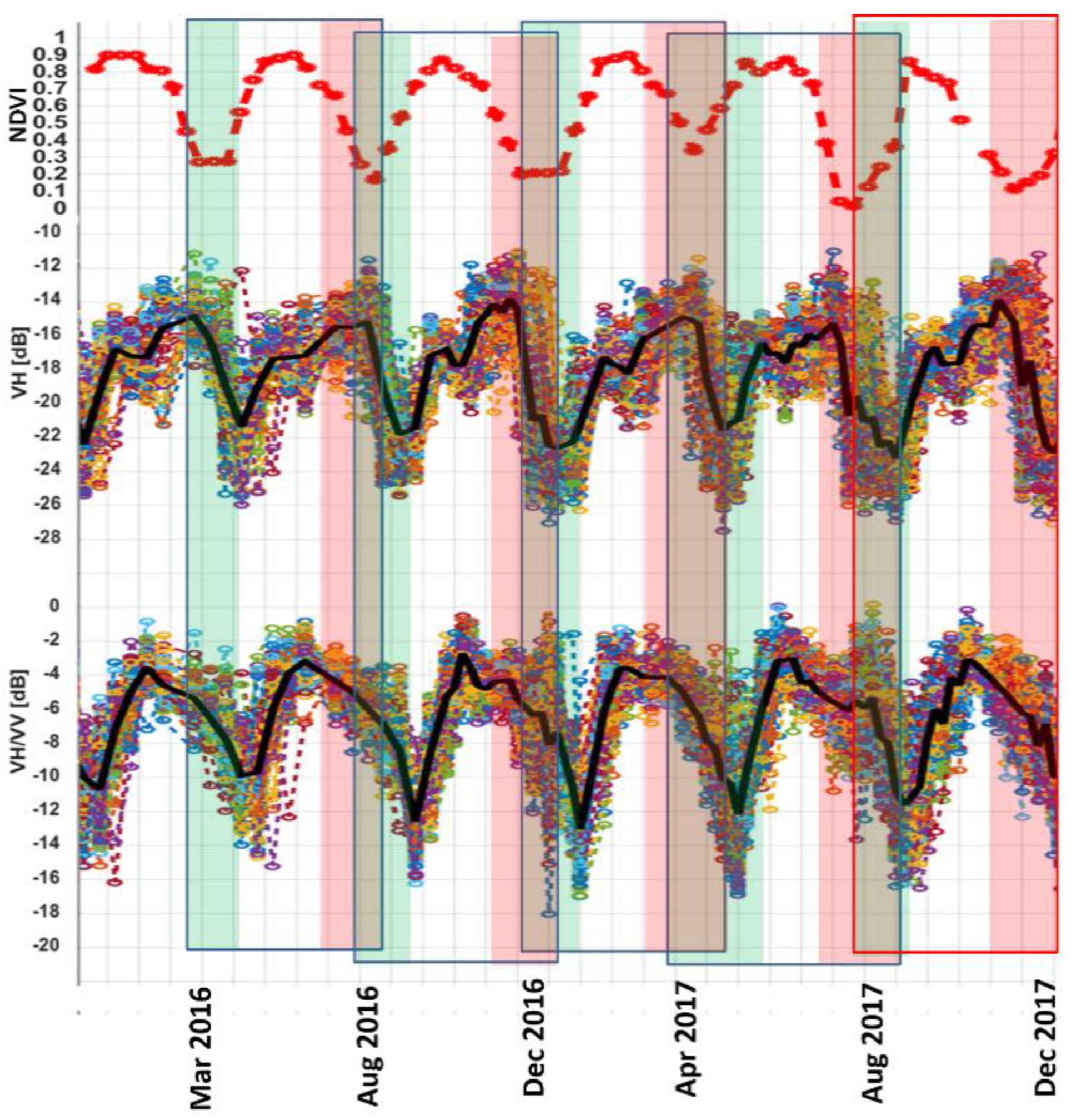
In order to further interpret the periodic patterns observed across seasons in Figure 9, in relation with the phenological stages, we compare the Sentinel-1 time series with optical data. Sentinel-2 (optical sensor) data are heavily affected by cloud cover in this region and could not be exploited. Instead, the 10-Day Syntheses (S10) of the coarser resolution (333 m) sensor Proba-V has been used. The Normalized Difference Vegetation Index (NDVI) images have been downloaded from http://www.vito-eodata.be/ (accessed on 20 April 2019). NDVI being an indicator of the amount of vegetation, it is not expected to distinguish easily rice from other vegetated land cover classes with periodic temporal patterns (e.g., other crops), however it can provide phenological information on areas previously identified as rice. The NDVI time series have been filtered to remove remaining clouds using an adaptation of the Best Index Slope Extraction (BISE) method [40]. Even after this cloud filtering in 10-day synthesis images, it was found that NDVI time series can be exploited for phenological analysis only over visually selected pixels, as many areas still have artefacts caused by cloud cover or represent mixed pixels. Figure 9 shows the average NDVI time series from January 2016 to December 2017 on the Proba-V pixels corresponding to the 60 rice fields under study, together with VH and VH/VV from Sentinel-1. Figure 9 shows the difference in the Sentinel-1 curves between 12 days or 6 days (after October 2016) acquisition intervals. In the second case, inter-season variation is better captured (in VV and VH), and the minimum backscatter values for each season are lower.

For the 60 fields with a diversity of conditions (varieties, cultural and irrigation practices, and environment conditions), the VH and VV mean backscatter temporal variation exhibits a specific pattern which is repeated for each cropping season over 5 years (Figure 8). From the start to the end of a rice season (indicated by vertical bars in Figure 9), neither VH nor VV exhibit a ‘bell curve’, as often suggested in past studies [23]. Instead, VH/VV follows well the bell curves, but the curves have their minima not at the start and the end of season but shifted about 20 days after the start of season. This behavior is to be compared with the NDVI curve, with minima ± 6 days after the sowing date and ± 6 days before the end of season.

3.2.4. Effect of Short/Long Cycle Duration, Effect of Water Management

The generic backscatter temporal behavior with respect to the phenological stage has been presented in Section 3.2.1. Here, we analyze the impact of other factors on this behavior. One important factor that introduces variability in the backscatter profiles was found to be the rice variety, in our study regrouped in long-cycle and short-cycle varieties.

Figure 10 shows the average values and standard deviations of VH, VV, and VH/VV backscatter over 4 growing seasons (Autumn–Winter 2016, Winter–Spring 2017, Autumn–Winter 2017 and Winter–Spring 2018) for 8 short-cycle rice fields (100 days duration, direct seeding) and 8 long-cycle rice fields (118 days duration, transplanting). The backscatter is plotted as a function of plant age (number of days after sowing).

Within each rice variety group, the VH and VV backscatter and polarization ratio VH/VV of the rice fields are very close to one another (less than 3 dB) during the entire rice cycle and their temporal variation can be interpreted as referred to the phenological stage.

When comparing the short cycle rice and long cycle rice groups, the main differences in the temporal evolution of VH, VV, and the ratio VH/VV can be summarized as follows:

• For the period before the start of season, VV and VH differ notably due to field preparation. For direct seeding, short cycle rice, fields are usually inundated for a few days to eliminate weeds, before drainage occurs, and direct seeding is done on wet soil. In the transplanting method associated to long cycle rice, fields are inundated just before transplantation. Moreover, as described in Section 3.1, the paddy fields of long cycle rice had very short recuperation periods (7–10 days) between two consecutive rice growing seasons. The maturity stage of rice of the previous rice season explains for the high backscatter values of long cycle rice in the period of -20 days to -10 days before the sowing date compared to short cycle rice where the rice fields were already harvested.
• At the beginning of the season, lower backscatter is observed in short cycle rice about 2–3 dB compared to long cycle rice. The direct seeding of short cycle rice is done on bare wet soil while the plants are already at 10–15 cm at transplantation for long cycle rice, this explains for this lower backscatter in short cycle rice. However, the differences between the backscatter curves are difficult to interpret either due to inundation status or due to rice varieties. For short cycle rice, for which the AWD method is applied, the duration of field inundation periods during the rice season is relatively short: 4–5 days at the beginning of the season, and before flowering. For the first flooding period, when the plants are small, the minimum backscatter is detected, but for the second period, when the plants are fully grown, the difference in backscatter with or without inundation is likely small (1–2 dB) and difficult to interpret. Moreover, with a repeat cycle of 6 day, it is not clear if Sentinel-1 can capture the field inundation states. For the long cycle rice, which is continuously flooded, at the start of the season, the plants are already at 10–15 cm at transplantation, the backscatter values are higher than that in short cycle rice, which is observed over several years.
• About 60 days after sowing, a clear difference between long and short cycle rice at VH and VV backscatter can be observed (Figure 10a,b). For short cycle rice, VH and VV start increasing after 60 days while for long cycle rice, they continue to decrease until 75 days then start increasing again.
• About 100 days after sowing, the VV and VH backscatter of short cycle rice decreases drastically, whereas the backscatter of long cycle rice continues its course.
• For VH/VV, the two rice types show quite similar temporal variations (Figure 10c) until the harvest of the short cycle rice.

3.2.5. Comparison between Cropping Systems

To distinguish rice from the other land use land cover (LULC) classes present in the region, it is important to understand the temporal variations of the backscatter of the other classes. Figure 11 shows the backscatter of the main other land cover classes present in the Mekong Delta, namely forest, water, and urban areas. All LULC types other than rice have a relatively stable backscatter and have very different VH and VV backscatter levels. Water surfaces have low VH and VV values because of the specular reflection. Forests (mostly Melaleuca plantations) and mango orchards have medium backscatter values and are stable in time. Corn fields (only a few in the region) show some variability, especially at VH, but with much higher backscatter than rice, similarly to what is observed in other regions, e.g., in Taiwan [41]. Urban areas have very high backscatter values.

The backscatter behavior of rice is distinctive in the following aspects:

• The VH backscatter has a large variability, and increases of about 10 dB in the season, from very low values (slightly higher than water) at the beginning of the season to high values shortly before harvest (Figure 11a).
• The VH/VV ratio is also very variable with a 10 dB dynamic range in the season from −13 dB to −3 dB, while it is remarkably stable in the −3 dB to −6 dB range for the other LULC classes (Figure 11c).

4. Discussion

Based on the backscatter profiles presented in the Results section, we can derive several indicators for rice mapping and rice parameters retrieval, which are discussed in the following subsections.

4.1. Rice Mapping

In line with previous findings, the particular temporal behavior of rice fields can be used to derive classification features.

Figure 11 shows that, in order to discriminate rice fields from other LULC, the specific temporal change of the VH backscatter and VH/VV ratio can be exploited. For example, the maximum increase observed in VH time series over a season can be used as a classification feature. In order to map a specific rice season, the time series needs to contain a date around the start or the end of the season, and a date approximately during the peak season (highest backscatter).

If the data at the beginning or the end of a given rice season are missed, for example because the limitation in handling a long time series of Sentinel-1 data, the maximum increase of the polarization ratio VH/VV is a better indicator than VH for rice field mapping. Because of its more complex temporal behavior along the season, the VV backscatter is less likely to provide a robust classification feature. However, information derived from both VV and VH polarizations (e.g., the maximum and minimum backscatter values in the time series of each polarization) can be used to map other land use/land cover classes (water, forest, built up area, other croplands) and therefore to mask out non-rice areas.

According to the repeated patterns observed across seasons in Figure 8, these patterns could be used as input in machine learning approaches, with the advantage of not requiring large amounts of training samples as in widely used supervised approach. However, for application at larger scales, the effect of incidence angle should be investigated, and an analysis similar to the one presented in this paper should be performed to assess the behavior of the backscatter of rice fields in relation to local specificities (cultural practices, rice varieties, comparison with other land use land cover, etc.).

4.2. Determination of Sowing Date

The trend of VH, VV, and VH/VV as a function of day after sowing presented in Figure 7bis confirmed in several rice seasons over several years (Figure 10) and can therefore be used as a reference curve to develop an indicator for sowing date estimation. At VH and VV polarizations, the confidence range of the reference curves is from 10 to 50 days after sowing where the radar backscatter behavior is the most stable without effect of long/short rice cycle rice variety or cultural practices. Curve-fitting methods could be applied to detect automatically the backscatter patterns corresponding to the period between 10 and 50 days after sowing, and therefore to derive the sowing date. Similarly, the VH/VV ratio reference curve over the whole rice cycle appears repeatable from one rice season to the other, with a decrease in the first 20 days followed by a 12–14 dB increase from 20 days after sowing until harvest, independently of the rice variety. This simple behavior and high dynamic range make the VH/VV time series a good candidate for sowing date estimation, for example through the estimation of the local minimum which occurs 20 days after sowing in the An Giang province. Again, for applications at larger scales, this behavior should be confirmed by local analyses.

The advantage of curve-fitting method is that it is based on the time series of Sentinel-1 over the rice growing cycle instead of exploiting a certain development stage of rice fields. This can minimize the effect of other parameters (incidence angle, climate condition, cultural practice, etc.). However, such a curve-fitting approach may require some prior knowledge of the local time frame during which sowing is likely to happen in order to restrict the analysis to shorter periods of time.

4.3. Mapping of Short/Long Cycle Rice

In Figure 10a,b the backscatter of the short cycle at around 65–75 days after sowing has lower backscatter values at both VH and VV polarizations as compared to the long cycle rice. A threshold method can be used as an indicator for the Sentinel-1 images during this period to distinguish long and short cycle rice varieties. This method therefore requires information of the sowing date obtained by the indicators developed in the previous subsection, and the results can be obtained only during the reproductive phase, from flowering stage to grain maturity phase.

To apply this method to other regions with different rice varieties, rice cycle duration, and cultural practices, the backscatter temporal behavior of the rice fields should be confirmed.

4.4. Phenological Stage Mapping

Figure 4 shows the range of dates, expressed as a number of days after sowing, at which each of the 12 phenological stages used by local authorities occur, both for short-cycle and long-cycle rice varieties. Once the sowing date is estimated, the phenological stage can therefore be derived for the rice fields in An Giang province, under the assumption that the plants follow their normal development. In Section 3.2.1, the backscatter temporal variation of Sentinel-1 data presented in Figure 7b has been interpreted as a function of the phenological stage. Consequently, at each growth stage, the VH, VV and VH/VV values can be used as indicators to confirm the rice growth development, for example using ranges of acceptable values for a given phenological stage.

To generalize the algorithms globally, more studies need to be carried out for diverse rice varieties and growth development from different regions. In particular, the knowledge of the duration of the rice growing season and the phenological development of rice plants are required, and the range of acceptable backscatter values for each growing stage need to be adapted to the incidence angle and cultural practices as described previously.

4.5. Plant Height

The analysis of plant height as a function of the day after sowing showed that the relationship can be expressed by polynomial regression curves with a high correlation coefficient (Figure 3). Two empirical polynomial regression curves, one for the short-cycle variety and one for the long-cycle variety, can be used as indicators for plant height estimation following the estimation of the sowing date. Again, the backscatter values at each date can be used to ensure that the field follows its normal development.

4.6. Production Timing

The indicators presented above can be applied in near-real time, with updates at each new Sentinel-1 acquisition. However, they can provide reliable information only after a certain delay after sowing:

• For rice mapping, it is possible to detect rice fields already at an early stage (less than 24 days after sowing), however such early detections must be confirmed with the next Sentinel-1 acquisitions.
• The sowing date can be estimated only after about 24 days (corresponding to 4 Sentinel-1 images of 6 days revisit), as it is necessary to wait until the VH/VV ratio reaches its minimum and start increasing again. When the sowing date is detected, the age of the plant can be calculated.
• The distinction between short and long cycle rice can be done after about 65 days, when the backscatter temporal profiles of the two groups start to differ.

5. Conclusions

The overall objective of this study was to analyze the backscatter temporal variation of rice fields, using Sentinel-1 and in-situ data from 2015 to 2020, in order to derive SAR-based indicators useful for rice monitoring applications.

For this purpose, data collected for the 5 rice seasons over 60 sampled fields in An Giang province have been used to interpret the Sentinel-1 backscatter temporal variation. Firstly, the analysis of the ground data showed that the crop calendars are not uniform within the region, leading to difficulties in obtaining information on the timing of the crop growth stages, in particular sowing and harvest dates. Most importantly, the analysis showed that during the rice cycle development, the plant structure changes at key phenological stages, in particular at the beginning of tillering (about 20 days after sowing) and at the booting-heading stage (about 60 days after sowing) when the rice plant loses its vertical structure, independently of the rice variety. Secondly, the temporal and polarization variations of the rice backscatter were interpreted with respect to physical interaction mechanisms to relate the backscatter dynamics (increasing, decreasing trends, and maximum and minimum values) to the key phenological stages, when the plants change their morphology and biomass. It was found that backscatter time series of rice fields show more complex patterns at VH and VV polarizations than the monotonic increase often reported in the past. As compared to other land use/land cover types, rice fields exhibit a very specific temporal behavior with a larger dynamic range. The analysis pointed out that the beginning of tillering and the booting-heading stages correspond to remarkable characteristics of the backscatter temporal curves (respectively minimum and maximum of the VH/VV curve). In particular, from 20 days after the start to the end of a rice season, VH/VV follows a bell curve, after its minimum at 20 days after sowing. The minimum value of VH is also found around 20 days after sowing while previous studies have claimed that this minimum indicated the start of season. The VH and VV mean backscatter temporal variation exhibits a specific pattern which is repeated for each cropping season over 5 years. Finally, these observations have led to the definition of Sentinel-1-based indicators that can be used to map rice, to estimate the sowing date and rice phenology, and to derive information such as the rice variety (long-cycle or short-cycle) and the plant height. The information of rice phenology and date of sowing is an asset for water management, field treatment and harvest planning and particularly useful to provide a synoptic view of the rice growth status over a region, which is difficult to have in a timely manner by ground survey.

However, to further interpret the rice backscatter temporal signature, there is a need to conduct electromagnetic modelling of the SAR signal. This would require a detailed description of the rice canopy by measuring geometric and dielectric properties of the rice plants and the rice canopy frequently, at least at each Sentinel-1 observation. Moreover, the indicators for rice mapping and monitoring developed in this study are based on the knowledge of the temporal development of the rice plants and the related temporal variation of the radar backscatter of different rice varieties and cultural practices over the An Giang province in the Mekong delta. In order to apply the algorithms to other regions under different conditions, for example rainfed, upland rice, etc., it is necessary to understand the backscatter temporal variations of the rice fields in order to refine the methods for their robustness across sites in other regions and countries. The analysis results presented in this paper will be used as a basis for rice monitoring programs using Sentinel-1 in the region.

References

1. Food Security. Rice in the Global Economy. Available online: https://agris.fao.org/agris-search/search.do?recordID=XF2015023402 (accessed on 20 April 2019).
2. Laborte, A.G.; Gutierrez, M.A.; Balanza, J.G.; Saito, K.; Zwart, S.J.; Boschetti, M.; Murty, M.; Villano, L.; Aunario, J.K.; Reinke, R.; et al. RiceAtlas, a spatial database of global rice calendars and production. Sci. Data 2017, 4, 1–10. [Google Scholar] [CrossRef] [PubMed]
3. North Africa and Latin America. PART 3 Feeding the World. 2007. Available online: http://www.fao.org/3/i2490e/i2490e03a.pdf (accessed on 20 April 2019).
4. IPCC. Methane Emissions from Rice cultivation: Flooded Rice Fields. In Revised 1996 IPCC Guidelines for National Greenhouse Gas Inventories Refinement; IPCC: Geneva, Switzerland, 1996; Volume 3, pp. 53–75. [Google Scholar]
5. Dong, J.; Xiao, X.; Menarguez, M.A.; Zhang, G.; Qin, Y.; Thau, D.; Biradar, C.; Moore, B., III. Mapping paddy rice planting area in northeastern Asia with Landsat 8 images, phenology-based algorithm and Google Earth Engine. Remote Sens. Environ. 2006, 185, 142–154. [Google Scholar] [CrossRef] [Green Version]
6. Kuenzer, C.; Knauer, K. Remote sensing of rice crop areas—A Review. Int. J. Remote Sens. 2013, 34, 2101–2139. [Google Scholar] [CrossRef]
7. Mosleh, M.K.; Hassan, Q.K.; Chowdhury, E.H. Application of Remote Sensors in Mapping Rice Area and Forecasting Its Production: A Review. Sensors 2015, 15, 769–791. [Google Scholar] [CrossRef] [Green Version]
8. Ferrant, S.; Selles, A.; Le Page, M.; Herrault, P.-A.; Pelletier, C.; Al-Bitar, A.; Mermoz, S.; Gascoin, S.; Bouvet, A.; Saqalli, M.; et al. Detection of Irrigated Crops from Sentinel-1 and Sentinel-2 Data to Estimate Seasonal Groundwater Use in South India. Remote Sens. 2017, 9, 1119. [Google Scholar] [CrossRef] [Green Version]
9. Torbick, N.; Chowdhury, D.; Salas, W.; Qi, J. Monitoring Rice Agriculture across Myanmar Using Time Series Sentinel-1 Assisted by Landsat-8 and PALSAR-2. Remote Sens. 2017, 9, 119. [Google Scholar] [CrossRef] [Green Version]
10. Lasko, K.; Vadrevu, K.P.; Tran, V.T.; Justice, C. Mapping Double and Single Crop Paddy Rice with Sentinel-1A at Varying Spatial Scales and Polarizations in Hanoi, Vietnam. IEEE J. Sel. Top. Appl. Earth Obs. Remote Sens. 2018, 11, 498–512. [Google Scholar] [CrossRef] [PubMed]
11. Ndikumana, E.; Minh, D.H.T.; Nguyen, H.T.D.; Baghdadi, N.; Courault, D.; Hossard, L.; El Moussawi, I. Estimation of Rice Height and Biomass Using Multitemporal SAR Sentinel-1 for Camargue, Southern France. Remote Sens. 2018, 10, 1394. [Google Scholar] [CrossRef] [Green Version]
12. Cai, Y.; Lin, H.; Zhang, M. Mapping paddy rice by the object-based random forest method using time series Sentinel-1/Sentinel-2 data. Adv. Space Res. 2019, 64, 2233–2244. [Google Scholar] [CrossRef]
13. De Castro Filho, H.C.; de Carvalho Júnior, O.A.; de Carvalho, O.L.F.; de Bem, P.P.; dos Santos de Moura, R.; de Albuquerque, A.O.; Rosa Silva, C.; Ferreira, P.H.G.; Guimaraes, R.F.; Trancoso Gomes, R.A. Rice crop detection using LSTM, Bi-LSTM, and machine learning models from Sentinel-1 time series. Remote Sens. 2020, 12, 2655. [Google Scholar] [CrossRef]
14. Mandal, D.; Kumar, V.; Bhattacharya, A.; Rao, Y.S.; Siqueira, P.; Bera, S. Sen4Rice: A Processing Chain for Differentiating Early and Late Transplanted Rice Using Time-Series Sentinel-1 SAR Data With Google Earth Engine. IEEE Geosci. Remote Sens. Lett. 2018, 15, 1947–1951. [Google Scholar] [CrossRef]
15. Tian, H.; Wu, M.; Wang, L.; Niu, Z. Mapping Early, Middle and Late Rice Extent Using Sentinel-1A and Landsat-8 Data in the Poyang Lake Plain, China. Sensors 2018, 18, 185. [Google Scholar] [CrossRef] [PubMed] [Green Version]
16. Le Toan, T.; Ribbes, F.; Wang, L.-F.; Floury, N.; Ding, K.-H.; Kong, J.A.; Fujita, M.; Kurosu, T. Rice crop mapping and monitoring using ERS-1 data based on experiment and modeling results. IEEE Trans. Geosci. Remote Sens. 1997, 35, 41–56. [Google Scholar] [CrossRef]
17. Le Toan, T.; Lam-Dao, N.; Apan, A.A.; Bouvet, A.; Young, F.; Le-Van, T. Effects of changing rice cultural practices on C-band synthetic aperture radar backscatter using Envisat advanced synthetic aperture radar data in the Mekong River Delta. J. Appl. Remote Sens. 2009, 3, 033563. [Google Scholar] [CrossRef] [Green Version]
18. Bouvet, A.; Le Toan, T. Use of ENVISAT/ASAR wide-swath data for timely rice fields mapping in the Mekong River Delta. Remote Sens. Environ. 2011, 115, 1090–1101. [Google Scholar] [CrossRef] [Green Version]
19. Nelson, A.; Setiyono, T.; Rala, A.B.; Quicho, E.D.; Raviz, J.V.; Abonete, P.J.; Maunahan, A.A.; Garcia, C.A.; Bhatti, H.Z.M.; Villano, L.S.; et al. Towards an Operational SAR-Based Rice Monitoring System in Asia: Examples from 13 Demonstration Sites across Asia in the RIICE Project. Remote Sens. 2014, 6, 10773–10812. [Google Scholar] [CrossRef] [Green Version]
20. Phan, H.; Le Toan, T.; Bouvet, A.; Nguyen, L.D.; Duy, T.P.; Zribi, M. Mapping of Rice Varieties and Sowing Date Using X-Band SAR Data. Sensors 2018, 18, 316. [Google Scholar] [CrossRef] [Green Version]
21. Clauss, K.; Ottinger, M.; Leinenkugel, P.; Kuenzer, C. Estimating rice production in the Mekong Delta, Vietnam, utilizing time series of Sentinel-1 SAR data. Int. J. Appl. Earth Obs. Geoinf. 2018, 73, 574–585. [Google Scholar] [CrossRef]
22. Phan, H.; Bouvet, A.; Le Toan, T. Sentinel-1 and Radarsat 2 data for rice monitoring in the Mekong delta, Vietnam. In Proceedings of the IGARSS 2015, Milan, Italy, 26–31 July 2015. [Google Scholar]
23. Nguyen, D.B.; Gruber, A.; Wagner, W. Mapping rice extent and cropping scheme in the Mekong Delta using Sentinel-1A data. Remote Sens. Lett. 2016, 7, 1209–1218. [Google Scholar] [CrossRef]
24. Dunn, A.M.; Hofmann, O.S.; Waters, B.; Witchel, E. Cloaking malware with the trusted platform module. In Proceedings of the 20th USENIX Security Symposium, San Francisco, CA, USA, 8–12 August 2011; pp. 395–410. [Google Scholar]
25. Zhan, P.; Zhu, W.; Li, N. Remote Sensing of Environment An automated rice mapping method based on flooding signals in synthetic aperture radar time series. Remote Sens. Environ. 2020, 252, 112112. [Google Scholar] [CrossRef]
26. Hoang-Phi, P.; Lam-Dao, N.; Pham-Van, C.; Chau-Nguyen-Xuan, Q.; Nguyen-Van-Anh, V.; Gummadi, S.; Le-Van, T. Sentinel-1 SAR Time Series-Based Assessment of the Impact of Severe Salinity Intrusion Events on Spatiotemporal Changes in Distribution of Rice Planting Areas in Coastal Provinces of the Mekong Delta, Vietnam. Remote Sens. 2020, 12, 3196. [Google Scholar] [CrossRef]
27. ESA. Available online: https://scihub.copernicus.eu/dhus/#/home (accessed on 26 September 2020).
28. Koleck, W.; Ballère, T.; Marie-Sainte, M. S1Tiling, A Multipurpose Open Source Processing Chain for Sentinel-1 Time Series. In Proceedings of the Living Planet, Milan, Italy, 13–17 May 2019. [Google Scholar]
29. CNES. Available online: https://peps.cnes.fr/ (accessed on 26 September 2020).
30. Shaun, Q.; Yu, J.J. Filtering of multichannel SAR images. IEEE Trans. Geosci. Remote Sens. 2001, 39, 2373–2379. [Google Scholar] [CrossRef]
31. Bruniquel, J.; Lopes, A. Multi-variate optimal speckle reduction in SAR imagery. Int. J. Remote Sens. 1997, 18, 603–627. [Google Scholar] [CrossRef]
32. FAO. Rice Market Monitor; FAO: Rome, Italy, 2017. [Google Scholar]
33. Picard, G.; Le Toan, T.; Mattia, F. Understanding c-band radar backscatter from wheat canopy using a multiple-scattering coherent model. IEEE Trans. Geosci. Remote Sens. 2003, 41, 1583–1591. [Google Scholar] [CrossRef]
34. Veloso, A.; Mermoz, S.; Bouvet, A.; Le Toan, T.; Planells, M.; Dejoux, J.-F.; Ceschia, E. Understanding the temporal behavior of crops using Sentinel-1 and Sentinel-2-like data for agricultural applications. Remote Sens. Environ. 2017, 199, 415–426. [Google Scholar] [CrossRef]
35. Koay, J.-Y.; Tan, C.-P.; Lim, K.-S.; Bin Abu Bakar, S.B.; Ewe, H.-T.; Chuah, H.-T.; Kong, J.-A. Paddy Fields as Electrically Dense Media: Theoretical Modeling and Measurement Comparisons. IEEE Trans. Geosci. Remote Sens. 2007, 45, 2837–2849. [Google Scholar] [CrossRef]
36. Inoue, Y.; Kurosu, T.; Maeno, H.; Uratsuka, S.; Kozu, T.; Dabrowska-Zielinska, K.; Qi, J. Season-long daily measurements of multifrequency (Ka, Ku, X, C, and L) and full-polarization backscatter signatures over paddy rice field and their relationship with biological variables. Remote Sens. Environ. 2002, 81, 194–204. [Google Scholar] [CrossRef]
37. Minasny, B.; Shah, R.M.; Soh, N.C.; Arif, C.; Setiawan, B.I. Automated Near-Real-Time Mapping and Monitoring of Rice Extent, Cropping Patterns, and Growth Stages in Southeast Asia Using Sentinel-1 Time Series on a Google Earth Engine Platform. Remote Sens. 2019, 11, 1666. [Google Scholar] [CrossRef] [Green Version]
38. Inoue, S.; Ito, A.; Yonezawa, C. Mapping Paddy Fields in Japan by Using a Sentinel-1 SAR Time Series Supplemented by Sentinel-2 Images on Google Earth Engine. Remote Sens. 2020, 12, 1622. [Google Scholar] [CrossRef]
39. Inoue, Y.; Sakaiya, E.; Wang, C. Capability of C-band backscattering coefficients from high-resolution satellite SAR sensors to assess biophysical variables in paddy rice. Remote Sens. Environ. 2014, 140, 257–266. [Google Scholar] [CrossRef]
40. Viovy, N.; Arino, O.; Belward, A.S. The Best Index Slope Extraction (BISE): A method for reducing noise in NDVI time-series. Int. J. Remote Sens. 1992, 13, 1585–1590. [Google Scholar] [CrossRef]
41. Chang, L.; Chen, Y.-T.; Wang, J.-H.; Chang, Y.-L. Rice-Field Mapping with Sentinel-1A SAR Time-Series Data. Remote Sens. 2020, 13, 103. [Google Scholar] [CrossRef]
Figure 1. The timetable of the data sets under study: collected ground data and Sentinel-1 data, along with the rice crop calendar in the An Giang province, Mekong Delta, Vietnam with three major cropping seasons: Winter–Spring (WS), Summer–Autumn (SA), and Autumn–Winter (AW).
Remotesensing 13 00921 g001
Figure 2. Example of Sentinel-1 image (descending pass) on 1st July 2020 in An Giang province (surrounded by purple line) in Mekong River Delta, Vietnam. The pixel grey tone indicates the radar backscattering coefficient in this VH image, black means low backscatter and white means high backscatter.
Remotesensing 13 00921 g002
Figure 3. Temporal variation of plant height (versus days after sowing): 15 sampling fields for long-cycle rice plants (blue points and black polynomial regression); 51 sampling fields for short-cycle rice plants (red points and pink polynomial regression) of 2 consecutive rice cropping seasons of Autumn–Winter 2017 and Winter–Spring 2018.
Remotesensing 13 00921 g003
Figure 4. Box-and-whisker plot of days of phenological stage (from 1 to 12, corresponding to the Scheme 51. short-cycle rice (red) and 15 sampling fields for long-cycle rice (blue) for the rice cropping seasons in Autumn–Winter 2017 and Winter–Spring 2018.
Remotesensing 13 00921 g004
Figure 5. Illustration of the rice fields under study at some phenological stages: (a) stage 1: sowing, (b) stage 3: beginning tillering, (c) stage 4: end of tillering, (d) stage 6: booting, (e) stage 8: flowering, (f) stage 10: milky stage.
Remotesensing 13 00921 g005
Figure 6. (a) Example of RGB combinations of different dates (R: 15th September 2017, G: 21st September 2017, B: 27th September 2017) from Sentinel-1 images VH polarization, (b) mean variation (black line) and standard deviation of VH, VV polarization ratio VH/VV extracted from Sentinel-1 images from August to December 2017 over 200 rice fields in the Mekong Delta.
Remotesensing 13 00921 g006
Figure 7. Temporal variation (the average of the 60 fields is in black line) and standard deviation of VH, VV polarization, ratio VH/VV extracted from Sentinel-1 images over 60 rice fields in the Autumn–Winter 2017 rice season as a function of Sentinel-1 acquisition date (a) and as a function of the number of days after sowing (b) and phenological stages.
Remotesensing 13 00921 g007
Figure 8. VH and VV backscatter coefficients and their ratio VH/VV extracted for the 60 sampled fields from Sentinel-1 images from 9th to 12th July 2020. It is noted that the revisit time of the Sentinel-1 (A+B) from 26th September 2016 is every 6 days. The black curves are the averaged quantities for all 60 fields.
Remotesensing 13 00921 g008
Figure 9. VH and ratio VH/VV extracted for the 60 sampled fields from Sentinel-1 images from January 2016 to December 2017 (the average of the 60 fields is in thick black line) compared with the NDVI time series (red curve) of the rice fields under study from January 2016 to December 2017. For each season, the sowing/transplanting and harvest periods are colored in green and red, respectively.
Remotesensing 13 00921 g009
Figure 10. Temporal evolutions and standard deviation of (a): VH, (b): VV, and (c): VH/VV of short rice cycle (green curves) and long rice cycle (blue curves) over 4 rice cropping seasons Autumn–Winter 2016, Winter–Spring 2017, Autumn–Winter 2017 and Winter–Spring 2018, with the period before sowing and after harvesting (black curves).
Remotesensing 13 00921 g010
Figure 11. Temporal evolutions and standard deviation of (a): VH, (b): VV, and (c): VH/VV backscatters of Sentinel-1 time series over rice fields (red), forest/tree (green), water body (blue), urban (purple), mango (brown), and corn (orange) from December 2019 to February 2020.
Remotesensing 13 00921 g011