
GECORIS: An Open-Source Toolbox for Analyzing Time Series of Corner Reflectors in InSAR Geodesy

Abstract
:
1. Introduction
- to present a standard procedure to analyze SAR time series of artificial radar reflectors to estimate their Radar Cross Section, Signal-to-Clutter Ratio and InSAR displacement time series,
- to implement this procedure into an efficient, open-source toolbox,
- to validate the performance of the developed toolbox on the networks of corner reflectors in Slovakia.
2. Theoretical Background
2.1. Radar Cross Section (RCS)
- ‘Integral’ estimation method [1,2,27]:where is the integrated power (intensity) in the mainlobe, corrected for the clutter power. Clutter power is estimated from four quadrants outside the cross-shaped area of the impulse response, assuming spatial ergodicity. is the relative power in the sidelobes and is the pixel area (not the resolution).
- ‘Peak’ estimation method [2,28]:where are the azimuth and range resolution respectively. In this method, the peak intensity is multiplied with the resolution cell area yielding the volume of a rectangular box, which is the same as the volume under an impulse response function. The peak intensity should be already corrected for the clutter and sensor noise. Alternatively, the clutter correction can be intentionally omitted here, obtaining the ‘apparent’ RCS. The clutter and the point scatter response can be later disentangled from the ‘apparent’ RCS by the temporal SCR estimation method [29].
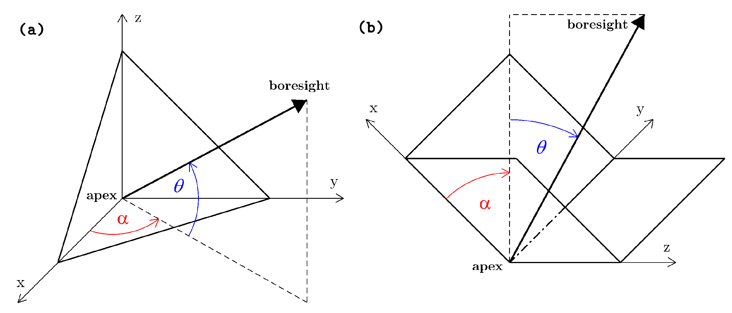
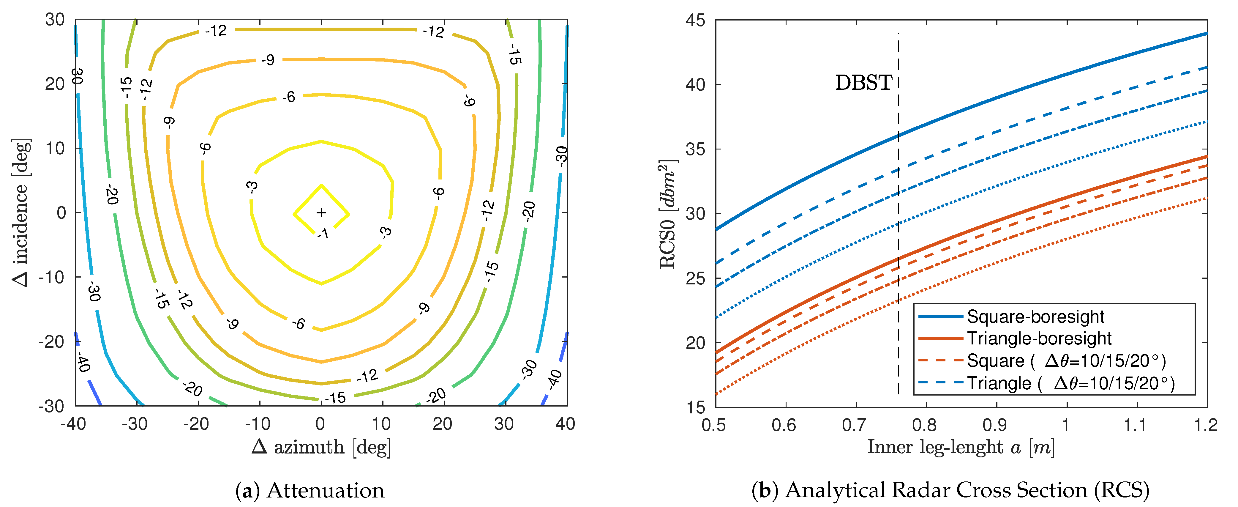
2.1.1. Analytical RCS
- inner-leg length dimension of a reflector is large with respect to a wavelength ;
- no implicit information on the reflector’s material is incorporated in the relations, only the presumption that it is homogeneous (e.g., three aluminium plates);
- reflector is in a ‘free-space’, absent of influence from surrounding objects, most notably the ground itself.
2.2. Signal-to-Clutter Ratio
2.3. SAR Positioning
- sub-pixel position of reflectors;
- datum differences;
- propagation effects;
- processing errors.
2.4. SAR Interferometry
3. Software Implementation
- Initial SAR time series analysis without the computationally demanding tasks, such as full SLC image co-registration, unnecessary for RCS and SCR estimation of reflectors. This is useful to operationally track the performance of an arbitrary number of reflectors within a local or regional network.
- Secondary full area analysis, including the InSAR time series analysis.
- The station log file, resembling ones typically used within permanent GNSS networks, such as International GNSS Service (IGS) [43]. It contains information on the reflector type, its geometry and orientation, coordinates of its phase centre for ascending/descending orbits, deployment and installation dates.
- The project parameters file, containing information on the SLC data stacks to be used within analysis.
- SLC data preparation.
- Positioning of reflectors in a radar datum.
- Reflector response extraction.
- Outlier detection.
- SCR estimation.
- InSAR time series analysis.
- Generation of plots, reports and data exchange files.
3.1. Data Preparation
- as raw measurements in their individual radar datum,
- as a co-registered stack, transformed onto a common geometric reference datum of an arbitrary master acquisition.
3.2. Network Design
3.3. Radar Positioning
Timing Corrections
- residual bistatic azimuth correction;
- Doppler-shift range correction;
- FM-rate mismatch azimuth correction.
3.4. Reflector Time Series Extraction
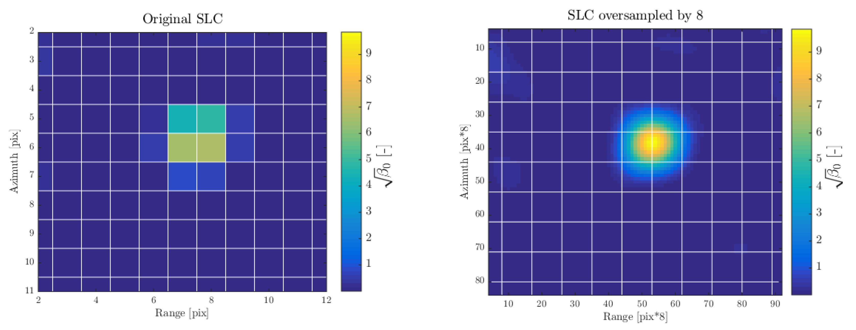
- A local maximum is identified in a small search window of 1 × 1 resolution cell around the initial reflector position in the oversampled data.
- Elliptic paraboloid is fitted in a smaller search window (9 × 9 subsampled pixels) centered on the maximum to refine the peak coordinates and amplitude estimate. This procedure guarantees the peak identification precision of 1/1000 pixel [9].
3.5. Outlier Detection
- 00
- no target or target disabled, no signal detected;
- 01
- no target or target disabled, but anomalous signal detected;
- 10
- target deployed/installed and/or enabled, but no signal detected;
- 11
- target deployed/installed and/or enabled, signal detected.
3.6. SCR Estimation
- the amplitude time series of the site, before the reflector was installed (i.e., with STATUS 00, see Section 3.5), are used to estimate the temporal average clutter power using a maximum likelihood fit of a Rayleigh distribution [37],
- the reflector’s peak amplitude time series (i.e., with STATUS 11, see Section 3.5) are used to estimate the temporal average of the reflector’s RCS and clutter power using a maximum likelihood fit of a Rice distribution [36],
- SCR estimate is finally obtained using Equation (5).
3.7. InSAR Network Solution
- CR and the PS candidates are connected using Delaunay triangulation to form a first-order estimation network.
- The phase correction due to the sub-pixel position [34] is evaluated for each CR.
- Variance Component Estimation (VCE) [60] is performed to obtain an initial diagonal variance-covariance matrix of the phase time series. A priori phase variances of CR are predicted using the estimated SCR (Section 3.6).
- The Atmospheric Phase Screen (APS) is estimated from the unwrapped phases using spatio-temporal filtering, variogram fitting and kriging interpolation [38].
- The unwrapped phase time series, corrected for the APS, are used to estimate the residual heights of the PS, using Equation (11) without the ambiguities.
- The phase residuals are then converted to the LOS displacement time series.
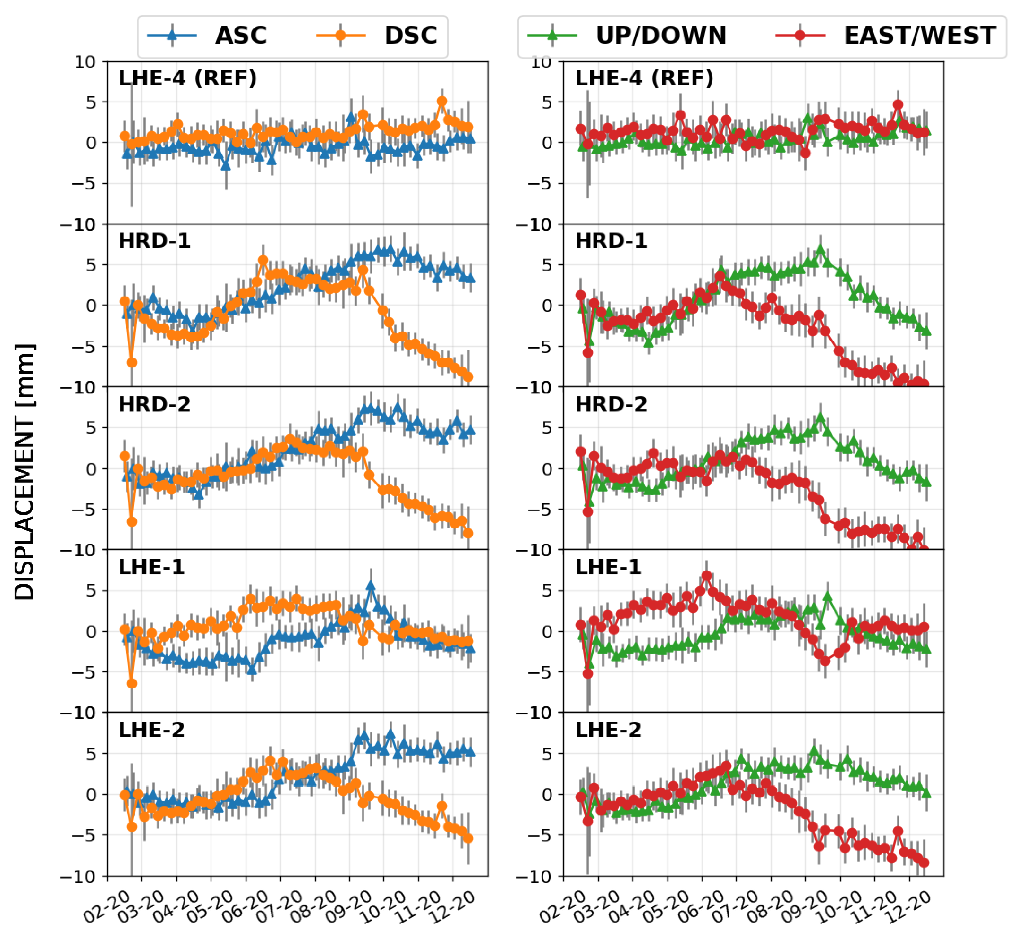
- Finally, decomposition of the cross-track LOS displacements of CR (see the double corner reflectors in Section 4.1) to the vertical and horizontal components is done by solving following linear equations [63]:where and are the ascending and descending displacements, and are the vertical and horizontal (approximately east-west) displacements, and are the local incidence angle and local azimuth angle, respectively. Full variance-covariance matrix of the vertical and horizontal displacements is obtained as:
4. Use Cases
4.1. Corner Reflector Network
4.1.1. Sentinel-1 Data
4.1.2. Design Considerations
- provide reliable displacement time series over the critical landslide zones,
- strengthen the PS estimation network,
- improve the positioning precision of the nearby PS,
- provide an absolute geodetic reference for the InSAR displacement estimates.
4.2. RCS Results
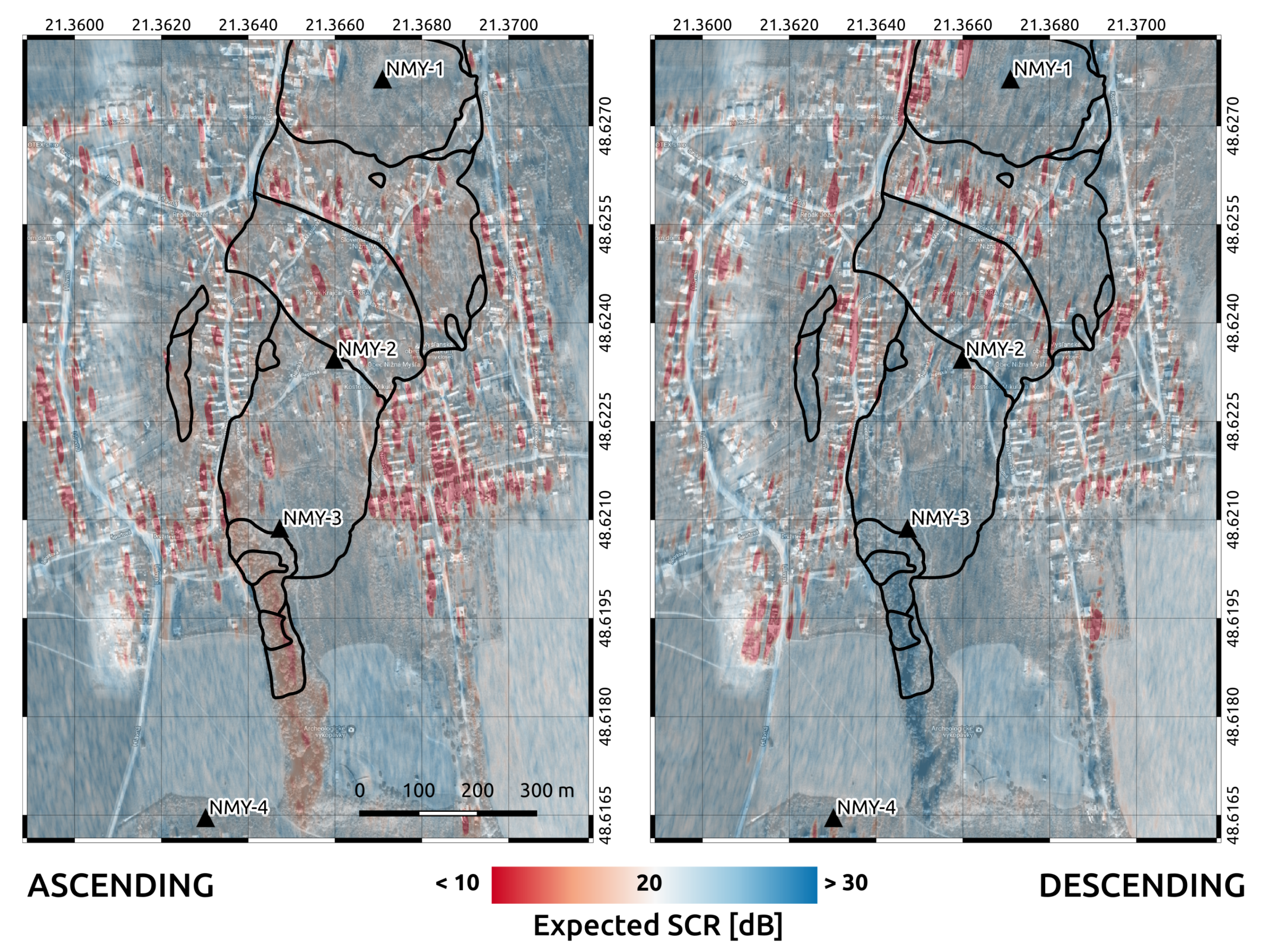
4.3. SCR Results
4.4. Precise SAR Positioning Results
4.5. InSAR Results
5. Discussion and Conclusions
- Support for other current SAR missions (e.g., Radarsat-2, TerraSAR-X).
- Support for corner reflectors of arbitrary shapes as well as radar transponders.
- Inclusion of repeated GNSS measurements of corner reflectors as auxiliary information to assist the spatio-temporal ambiguity resolution within the InSAR processing.
- Incorporating a corner reflector as a PS with known absolute position in the TRF, fixing the relative height estimates of the nearby PS [18].
Author Contributions
Funding
Institutional Review Board Statement
Informed Consent Statement
Data Availability Statement
Acknowledgments
Conflicts of Interest
Abbreviations
| FOSS | Free and Open-Source Software |
| CR | Corner Reflector/Reflectors |
| SAR | Synthetic Aperture Radar |
| InSAR | Interferometric Synthetic Aperture Radar |
| RCS | Radar Cross Section |
| SCR | Signal-to-Clutter Ratio |
| TRF | Terrestrial Reference Frame |
| ITRS | International Terrestrial Reference System |
| ETRS89 | European Terrestrial Reference System |
| ITRF | International Terrestrial Reference Frame |
| SET | Solid Earth Tides |
| PS | Point Scatterer |
| GNSS | Global Navigation Satellite Systems |
| IRF | Impulse Response Function |
| SLC | Single Look Complex |
| IWS | Interferometric Wide Swath |
| LOS | Line-of-Sight |
| DBST | Double Back-flipped Square Trihedral |
| PRF | Pulse Repetition Frequency |
| RSR | Range Sampling Rate |
| CRLB | Cramer-Rao Lower Bound |
| APS | Atmospheric Phase Screen |
| SNAP | Sentinels Application Platform |
| IGS | International GNSS Service |
| EUREF | Reference Frame Subcommission for Europe |
| ECMWF | European Centre for Medium-Range Weather Forecasts |
| TEC | Total Electron Content |
| TOPS | Terrain Observation with Progressive Scan |
| MAD | Median Absolute Deviation |
| VCE | Variance Component Estimation |
| APE | Absolute Positioning Error |
| DLR | Deutsches Zentrum für Luft |
References
- Freeman, A. SAR calibration: An overview. IEEE Trans. Geosci. Remote Sens. 1992, 30, 1107–1121. [Google Scholar] [CrossRef]
- Gray, A.; Vachon, P.; Livingstone, C.; Lukowski, T. Synthetic aperture radar calibration using reference reflectors. IEEE Trans. Geosci. Remote Sens. 1990, 28, 374–383. [Google Scholar] [CrossRef]
- Doerry, A.W. Reflectors for SAR Performance Testing; Technical Report; Sandia National Laboratories: Albuquerque, NM, USA; Livermore, CA, USA, 2008.
- CLS. Sentinel-1A N-Cyclic Performance Report—2020-07; Technical Report 7; Collecte Localisation Satellites (CLS): Ramonville Saint-Agne, France, 2020. [Google Scholar]
- CLS. Sentinel-1B N-Cyclic Performance Report—2020-07; Technical Report 7; Collecte Localisation Satellites (CLS): Ramonville Saint-Agne, France, 2020. [Google Scholar]
- Prati, C.; Rocca, F.; Monti Guarnieri, A. SAR interferometry experiments with ERS-1. In Proceedings of the First ERS-1 Symposium—Space at the Service of our Environment, Cannes, France, 4–6 November 1992; pp. 211–217. [Google Scholar]
- Marinkovic, P.; Ketelaar, V.; van Leijen, F.; Hanssen, R. InSAR Quality Control: Analysis of Five Years of Corner Reflector Time Series. In Proceedings of the Fifth International Workshop on ERS/Envisat SAR Interferometry, ‘FRINGE07’, Frascati, Italy, 26–30 November 2007; Lacoste, H., Ouwehand, L., Eds.; ESA Communication Production Office: Noordwijk, The Netherlands, 2008; pp. 1–8. [Google Scholar]
- Schubert, A.; Miranda, N.; Geudtner, D.; Small, D. Sentinel-1A/B Combined Product Geolocation Accuracy. Remote Sens. 2017, 9, 607. [Google Scholar] [CrossRef] [Green Version]
- Balss, U.; Gisinger, C.; Eineder, M.; Breit, H.; Schubert, A.; Small, D. Survey Protocol for Geometric SAR Sensor Analysis; Technical Report; German Aerospace Center (DLR), Technical University of Munich (TUM), Remote Sensing Laboratories—University of Zurich (RSL): Oberpfaffenhofen, Germany, 2018. [Google Scholar]
- Gisinger, C.; Schubert, A.; Breit, H.; Garthwaite, M.; Balss, U.; Willberg, M.; Small, D.; Eineder, M.; Miranda, N. In-Depth Verification of Sentinel-1 and TerraSAR-X Geolocation Accuracy Using the Australian Corner Reflector Array. IEEE Trans. Geosci. Remote Sens. 2020, 1–28. [Google Scholar] [CrossRef]
- Garthwaite, M.C. On the Design of Radar Corner Reflectors for Deformation Monitoring in Multi-Frequency InSAR. Remote Sens. 2017, 9, 648. [Google Scholar] [CrossRef] [Green Version]
- Jauvin, M.; Yan, Y.; Trouvé, E.; Fruneau, B.; Gay, M.; Girard, B. Integration of Corner Reflectors for the Monitoring of Mountain Glacier Areas with Sentinel-1 Time Series. Remote Sens. 2019, 11, 988. [Google Scholar] [CrossRef] [Green Version]
- Mahapatra, P.; van der Marel, H.; van Leijen, F.; Samiei Esfahany, S.; Klees, R.; Hanssen, R. InSAR datum connection using GNSS-augmented radar transponders. J. Geod. 2017. [Google Scholar] [CrossRef] [Green Version]
- Bamler, R.; Hartl, P. Synthetic aperture radar interferometry. Inverse Probl. 1998, 14, R1–R54. [Google Scholar] [CrossRef]
- Cumming, I.G.; Wong, F.H. Digital Processing of Synthetic Aperture Radar Data: Algorithms and Implementation; Artech House: London, UK, 2005; Volume 1. [Google Scholar]
- Dheenathayalan, P.; Small, D.; Schubert, A.; Hanssen, R.F. High-precision positioning of radar scatterers. J. Geod. 2016, 90, 403–422. [Google Scholar] [CrossRef] [Green Version]
- Gisinger, C.; Willberg, M.; Balss, U.; Klügel, T.; Mähler, S.; Pail, R.; Eineder, M. Differential geodetic stereo SAR with TerraSAR-X by exploiting small multi-directional radar reflectors. J. Geod. 2016, 91. [Google Scholar] [CrossRef]
- Yang, M.; López-Dekker, P.; Dheenathayalan, P.; Liao, M.; Hanssen, R.F. On the value of corner reflectors and surface models in InSAR precise point positioning. ISPRS J. Photogramm. Remote Sens. 2019, 158, 113–122. [Google Scholar] [CrossRef]
- Dheenathayalan, P.; Cuenca, M.C.; Hoogeboom, P.; Hanssen, R.F. Small reflectors for ground motion monitoring with InSAR. IEEE Trans. Geosci. Remote Sens. 2017, 55, 6703–6712. [Google Scholar] [CrossRef]
- Bamler, R.; Eineder, M. Accuracy of differential shift estimation by correlation and split-bandwidth interferometry for wideband and delta-k SAR systems. IEEE Geosci. Remote Sens. Lett. 2005, 2, 151–155. [Google Scholar] [CrossRef]
- Garthwaite, M.C.; Nancarrow, S.; Hislop, A.; Thankappan, M.; Dawson, J.H.; Lawrie, S. The Design of Radar Corner Reflectors for the Australian Geophysical Observing System: A Single Design Suitable for InSAR Deformation Monitoring and SAR Calibration at Multiple Microwave Frequency Bands; Technical Report; Geoscience Australia: Canberra, Australia, 2015. [CrossRef]
- Hanssen, R.F. A Radar Retroreflector Device and a Method of Preparing a Radar Retroreflector Device. WO/2018/236215, 27 December 2018. [Google Scholar]
- Kamphuis, J. Co-Location of Geodetic Reference Points. Master’s Thesis, TU Delft Civil Engineering and Geoscience, Delft, The Netherlands, 2019. [Google Scholar]
- Raney, R.K.; Freeman, T.; Hawkins, R.W.; Bamler, R. A plea for radar brightness. In Proceedings of the IGARSS’94—1994 IEEE International Geoscience and Remote Sensing Symposium, Pasadena, CA, USA, 8–12 August 1994; Volume 2, pp. 1090–1092. [Google Scholar]
- Radiometric Calibration of S-1 Level-1 Products Generated by the S-1 IPF; ESA-EOPG-CSCOP-TN-0002. Technical Report. 2015. Available online: https://sentinel.esa.int/documents/247904/685163/S1-Radiometric-Calibration-V1.0.pdf (accessed on 22 February 2021).
- Skolnik, M. Introduction to Radar Systems; Electrical Engineering Series; McGraw-Hill: Singapore, 2001. [Google Scholar]
- Schmidt, K.; Schwerdt, M.; Miranda, N.; Reimann, J. Radiometric Comparison within the Sentinel-1 SAR Constellation over a Wide Backscatter Range. Remote Sens. 2020, 12, 854. [Google Scholar] [CrossRef] [Green Version]
- Ulander, L.M. Accuracy of Using Point Targets for SAR Calibration. IEEE Trans. Aerosp. Electron. Syst. 1991, 27, 139–148. [Google Scholar] [CrossRef]
- Czikhardt, R.; van der Marel, H.; van Leijen, F.J.; Hanssen, R.F. Estimating Signal-to-Clutter Ratio of InSAR Corner Reflectors from SAR Time Series. IEEE Geosci. Remote Sens. Lett. 2021. submitted. [Google Scholar]
- Groot, J. Letter: Cross Section Computation of Trihedral Corner Reflectors with the Geometrical Optics Approximation. Eur. Trans. Telecommun. 1992, 3, 637–642. [Google Scholar] [CrossRef]
- Qin, Y.; Perissin, D.; Lei, L. The Design and Experiments on Corner Reflectors for Urban Ground Deformation Monitoring in Hong Kong. Int. J. Antennas Propag. 2013, 2013. [Google Scholar] [CrossRef] [Green Version]
- Van der Marel, H.; van Leijen, F.J.; Hanssen, R.F. First Analysis of C-Band ECR Transponders for Insar Geodesy. In Proceedings of the IGARSS 2018—2018 IEEE International Geoscience and Remote Sensing Symposium, Valencia, Spain, 22–27 July 2018; pp. 1399–1402. [Google Scholar] [CrossRef] [Green Version]
- Guide to Sentinel-1 Geocoding; Technical Report; Remote Sensing Laboratories—University of Zurich (RSL). 2019. Available online: https://sentinel.esa.int/documents/247904/1653442/Guide-to-Sentinel-1-Geocoding.pdf (accessed on 22 February 2021).
- Yang, M.; Dheenathayalan, P.; López-Dekker, P.; van Leijen, F.; Liao, M.; Hanssen, R.F. On the influence of sub-pixel position correction for PS localization accuracy and time series quality. ISPRS J. Photogramm. Remote Sens. 2020, 165, 98–107. [Google Scholar] [CrossRef]
- Balss, U.; Gisinger, C.; Eineder, M. Measurements on the Absolute 2-D and 3-D Localization Accuracy of TerraSAR-X. Remote Sens. 2018, 10, 656. [Google Scholar] [CrossRef] [Green Version]
- Ferretti, A.; Prati, C.; Rocca, F. Permanent Scatterers in SAR Interferometry. IEEE Trans. Geosci. Remote Sens. 2001, 39, 8–20. [Google Scholar] [CrossRef]
- Hanssen, R.F. Radar Interferometry: Data Interpretation and Error Analysis; Springer: Berlin/Heidelberg, Germany, 2001; Volume 2. [Google Scholar]
- Van Leijen, F.J. Persistent Scatterer Interferometry Based on Geodetic Estimation Theory; NCG: Amersfoort, The Netherlands, 2014. [Google Scholar]
- Ansari, H.; De Zan, F.; Bamler, R. Efficient Phase Estimation for Interferogram Stacks. IEEE Trans. Geosci. Remote Sens. 2018, 56, 4109–4125. [Google Scholar] [CrossRef]
- Hu, F.; Wu, J.; Chang, L.; Hanssen, R. Incorporating Temporary Coherent Scatterers in Multi-Temporal InSAR Using Adaptive Temporal Subsets. IEEE Trans. Geosci. Remote Sens. 2019, 1–13. [Google Scholar] [CrossRef] [Green Version]
- Kampes, B.M.; Hanssen, R.F. Ambiguity Resolution for Permanent Scatterer Interferometry. IEEE Trans. Geosci. Remote Sens. 2004, 42, 2446–2453. [Google Scholar] [CrossRef] [Green Version]
- ESA. Sentinel Application Platform (SNAP). Available online: https://step.esa.int/main/toolboxes/snap/ (accessed on 22 February 2021).
- IGS. International GNSS Service. Available online: http://www.igs.org/ (accessed on 22 February 2021).
- EUREF. Reference Frame Sub-Commission for Europe. Available online: http://www.euref.eu (accessed on 22 February 2021).
- Sansosti, E.; Berardino, P.; Manunta, M.; Serafino, F.; Fornaro, G. Geometrical SAR image registration. IEEE Trans. Geosci. Remote Sens. 2006, 44, 2861–2870. [Google Scholar] [CrossRef]
- Prats-Iraola, P.; Scheiber, R.; Marotti, L.; Wollstadt, S.; Reigber, A. TOPS Interferometry With TerraSAR-X. IEEE Trans. Geosci. Remote Sens. 2012, 50, 3179–3188. [Google Scholar] [CrossRef] [Green Version]
- Czikhardt, R.; Papco, J.; Bakon, M.; Liscak, P.; Ondrejka, P.; Zlocha, M. Ground Stability Monitoring of Undermined and Landslide Prone Areas by Means of Sentinel-1 Multi-Temporal InSAR, Case Study from Slovakia. Geosciences 2017, 7, 87. [Google Scholar] [CrossRef] [Green Version]
- Peter, H.; Jäggi, A.; Fernández, J.; Escobar, D.; Ayuga, F.; Arnold, D.; Wermuth, M.; Hackel, S.; Otten, M.; Simons, W.; et al. Sentinel-1A—First precise orbit determination results. Adv. Space Res. 2017, 60, 879–892. [Google Scholar] [CrossRef]
- EUREF Technical Note 1: Relationship and Transformation between the International and the European Terrestrial Reference Systems. Technical Report. 2018. Available online: http://etrs89.ensg.ign.fr/pub/EUREF-TN-1.pdf (accessed on 22 February 2021).
- IERS. International Earth Rotation and Reference Systems Service. Available online: https://www.iers.org/ (accessed on 22 February 2021).
- Hersbach, H.; Dee, D. ERA5 reanalysis is in production. ECMWF Newsl. 2016, 147, 5–6. [Google Scholar]
- Hu, Z.; Mallorquí, J.J. An Accurate Method to Correct Atmospheric Phase Delay for InSAR with the ERA5 Global Atmospheric Model. Remote Sens. 2019, 11, 1969. [Google Scholar] [CrossRef] [Green Version]
- CLS. Sentinel-1 Level 1 Detailed Algorithm Definition; Technical Report; Collecte Localisation Satellites (CLS): Ramonville Saint-Agne, France, 2019. [Google Scholar]
- Yague-Martinez, N.; De Zan, F.; Prats-Iraola, P. Coregistration of Interferometric Stacks of Sentinel-1 TOPS Data. IEEE Geosci. Remote Sens. Lett. 2017, 14, 1002–1006. [Google Scholar] [CrossRef] [Green Version]
- Definition of the TOPS SLC Deramping Function for Products Generated by the S-1 IPF, 3rd ed.; European Space Agency: Paris, France, 2017; Available online: https://earth.esa.int/documents/247904/1653442/Sentinel-1-TOPS-SLC_Deramping (accessed on 22 February 2021).
- Leys, C.; Ley, C.; Klein, O.; Bernard, P.; Licata, L. Detecting outliers: Do not use standard deviation around the mean, use absolute deviation around the median. J. Exp. Soc. Psychol. 2013, 49, 764–766. [Google Scholar] [CrossRef] [Green Version]
- Ketelaar, G.; Marinkovic, P.; Hanssen, R. Validation of point scatterer phase statistics in multi-pass InSAR. In Proceedings of the CEOS SAR Workshop, Ulm, Germany, 27–28 May 2004; pp. 27–28. [Google Scholar]
- Chum, O.; Philbin, J.; Zisserman, A. Near duplicate image detection: Min-Hash and tf-idf weighting. In Proceedings of the 19th British Machine Vision Conference (BMVC 2008), Leeds, UK, 1–4 September 2008; pp. 812–815. [Google Scholar]
- Perissin, D. SAR Super-Resolution and Characterization of Urban Targets: An Advanced Analysis on the Physical Nature of Synthetic Aperture Radar Permanent Scatterers through ERS and Envisat Interferometry; VDM Verlag Dr. Müller: Saarbrücken, Germany, 2010. [Google Scholar]
- Teunissen, P.J.G.; Amiri-Simkooei, A.R. Least-squares variance component estimation. J. Geod. 2008, 82, 65–82. [Google Scholar] [CrossRef] [Green Version]
- Teunissen, P.J.G. Least-Squares Estimation of the Integer GPS Ambiguities: LRS Series 6; Technical Report; Delft Geodetic Computing Centre, Delft University of Technology: Delft, The Netherlands, 1993. [Google Scholar]
- Kampes, B.M. Radar Interferometry: Persistent Scatterer Technique; Springer: Berlin/Heidelberg, Germany, 2006. [Google Scholar]
- Ketelaar, V.B.H.G. Satellite Radar Interferometry: Subsidence Monitoring Techniques; Springer: Assen, The Netherlands, 2009. [Google Scholar] [CrossRef]
- SKPOS. Slovak Real Time Positioning Service. Available online: http://www.skpos.gku.sk/en/ (accessed on 22 February 2021).
- Bakon, M.; Czikhardt, R.; Papco, J.; Barlak, J.; Rovnak, M.; Adamisin, P.; Perissin, D. remotIO: A Sentinel-1 Multi-Temporal InSAR Infrastructure Monitoring Service with Automatic Updates and Data Mining Capabilities. Remote Sens. 2020, 12, 1892. [Google Scholar] [CrossRef]
- Ondrejka, P.; Bakon, M.; Papco, J.; Liscak, P. Monitoring of sliding activity of the territory Prievidza-Hradec. Geotechnika 2016, 2016, 3–12, (In Slovak with English summary). [Google Scholar]
- Barzaghi, R.; Reguzzoni, M.; De Gaetani, C.; Caldera, S.; Rossi, L. Cultural Heritage Monitoring by Low-cost GNSS Receivers: A Feasibility Study for San Gaudenzio’s Cupola, Novara. ISPRS Int. Arch. Photogramm. Remote Sens. Spat. Inf. Sci. 2019, XLII-2/W11, 209–216. [Google Scholar] [CrossRef] [Green Version]
- Teunissen, P. Zero order design: Generalized inverses, adjustment, the datum problem and S-transformations. In Optimization and Design of Geodetic Networks; Springer: Berlin/Heidelberg, Germany, 1985; pp. 11–55. [Google Scholar]


| CR | Sentinel-1 | RCS [dBm2] | SCR [dB] | ||||
|---|---|---|---|---|---|---|---|
| Track | Predic. | Estim. | [dBm2] | Predic. | Estim. | [mm] | |
| HRD-1 | ASC175 | 33.57 | 32.88 | 0.29 | 26.69 | 24.42 | 0.27 |
| DSC51 | 33.48 | 32.57 | 0.29 | 28.30 | 24.27 | 0.27 | |
| HRD-2 | ASC175 | 33.57 | 33.05 | 0.31 | 25.78 | 23.97 | 0.28 |
| DSC51 | 33.47 | 32.50 | 0.37 | 26.87 | 22.35 | 0.34 | |
| LHE-1 | ASC175 | 33.57 | 33.00 | 0.30 | 27.90 | 24.18 | 0.28 |
| DSC51 | 33.47 | 32.96 | 0.37 | 24.65 | 22.20 | 0.35 | |
| LHE-2 | ASC175 | 33.57 | 33.22 | 0.39 | 23.14 | 21.74 | 0.37 |
| DSC51 | 33.47 | 32.83 | 0.27 | 28.66 | 25.05 | 0.25 | |
| LHE-4 | ASC175 | 33.57 | 33.19 | 0.32 | 25.38 | 23.68 | 0.29 |
| DSC51 | 33.47 | 32.84 | 0.32 | 23.97 | 23.61 | 0.29 | |
| CR | Sentinel-1 | Azimuth [m] | Range [m] | ||
|---|---|---|---|---|---|
| track | CRLB | APE | CRLB | APE | |
| HRD-1 | ASC175 | 0.51 | −0.21 ± 0.76 | 0.07 | −0.02 ± 0.16 |
| DSC51 | 0.52 | 0.19 ± 0.50 | 0.08 | −0.08 ± 0.16 | |
| HRD-2 | ASC175 | 0.54 | 0.64 ± 0.72 | 0.08 | −0.02 ± 0.14 |
| DSC51 | 0.65 | 0.44 ± 0.56 | 0.10 | −0.12 ± 0.18 | |
| LHE-1 | ASC175 | 0.53 | 0.12 ± 0.57 | 0.07 | 0.03 ± 0.18 |
| DSC51 | 0.66 | 0.29 ± 0.89 | 0.11 | −0.15 ± 0.20 | |
| LHE-2 | ASC175 | 0.70 | 0.31 ± 0.74 | 0.10 | −0.02 ± 0.21 |
| DSC51 | 0.47 | 0.06 ± 0.58 | 0.08 | −0.10 ± 0.16 | |
| LHE-4 | ASC175 | 0.56 | 0.38 ± 0.66 | 0.08 | 0.02 ± 0.19 |
| DSC51 | 0.56 | 0.17 ± 0.62 | 0.09 | −0.13 ± 0.17 | |
Publisher’s Note: MDPI stays neutral with regard to jurisdictional claims in published maps and institutional affiliations. |
© 2021 by the authors. Licensee MDPI, Basel, Switzerland. This article is an open access article distributed under the terms and conditions of the Creative Commons Attribution (CC BY) license (http://creativecommons.org/licenses/by/4.0/).
Share and Cite
Czikhardt, R.; van der Marel, H.; Papco, J. GECORIS: An Open-Source Toolbox for Analyzing Time Series of Corner Reflectors in InSAR Geodesy. Remote Sens. 2021, 13, 926. https://doi.org/10.3390/rs13050926
Czikhardt R, van der Marel H, Papco J. GECORIS: An Open-Source Toolbox for Analyzing Time Series of Corner Reflectors in InSAR Geodesy. Remote Sensing. 2021; 13(5):926. https://doi.org/10.3390/rs13050926
Chicago/Turabian StyleCzikhardt, Richard, Hans van der Marel, and Juraj Papco. 2021. "GECORIS: An Open-Source Toolbox for Analyzing Time Series of Corner Reflectors in InSAR Geodesy" Remote Sensing 13, no. 5: 926. https://doi.org/10.3390/rs13050926