Impact of Tree Crown Transmittance on Surface Reflectance Retrieval in the Shade for High Spatial Resolution Imaging Spectroscopy: A Simulation Analysis Based on Tree Modeling Scenarios

Abstract

With the advancement of high spatial resolution imaging spectroscopy, an accurate surface reflectance retrieval is needed to derive relevant physical variables for land cover mapping, soil, and vegetation monitoring. One challenge is to deal with tree shadows using atmospheric correction models if the tree crown transmittance $T_c$ is not properly taken into account. This requires knowledge of the complex radiation mechanisms that occur in tree crowns, which can be provided by coupling the physical modeling of canopy radiative transfer codes (here DART) and the 3D representations of trees. First in this study, a sensitivity analysis carried out on DART simulations with an empirical 3D tree model led to a statistical regression predicting $T_c$ from the tree leaf area index (LAI) and the solar zenith angle with good performances (RMSE ≤ 4.3% and R² ≥ 0.91 for LAI ≤ 4 m².m⁻²). Secondly, more realistic 3D voxel-grid tree models derived from terrestrial LiDAR measurements over two trees were considered. The comparison of DART-simulated $T_c$ from these models with the previous predicted $T_c$ over 0.4–2.5 µm showed three main sources of inaccuracy quoted in order of importance: (1) the global tree geometry shape (mean bias up to 21.5%), (2) the transmittance fraction associated to multiple scattering, $T_{scat}$ (maximum bias up to 13%), and (3) the degree of realism of the tree representation (mean bias up to 7.5%). Results showed that neglecting $T_c$ leads to very inaccurate reflectance retrieval (mean bias > 0.04), particularly if the background reflectance is high, and in the near and shortwave infrared – NIR and SWIR – due to $T_{scat}$. The transmittance fraction associated to the non-intercepted transmitted light, $T_{dir}$, can reach up to 95% in the SWIR, and $T_{scat}$ up to 20% in the NIR. Their spatial contributions computed in the tree shadow have a maximum dispersion of 27% and 8% respectively. Investigating how to approximate $T_{dir}$ and $T_{scat}$ spectral and spatial variability along with the most appropriate tree 3D modeling is crucial to improve reflectance retrieval in tree shadows when using atmospheric correction models.

1. Introduction

The use of imaging spectroscopy (IS) compared to multispectral imagery has opened the way to providing access to more physical surface properties for better monitoring of land cover mapping, vegetation, and soil monitoring in both urban and natural ecosystems [1,2,3]. However, their derivation requires accurate surface reflectance retrieval. For instance, erroneous surface reflectances lead to incorrect calculation of vegetation indices and, later, to a spurious assessment of vegetation biochemical and biophysical properties [4,5,6]. With the advancement of high spatial resolution IS, such as operated by airborne and UAV platforms, the major issue is the presence of shadows either cast by manmade infrastructures or trees. In an urban context composed of buildings and a tree-covered park, Adeline et al. [7] showed that the proportion of shadows can account around between 20% and 30% of the image pixels for a zenith angle of 32° at an airborne spatial resolution of 0.2 m. Then, in many cases, shadows are masked or considered as a class by their own for further applications, but this is to the detriment to process the whole image if, for instance, the objects of interest are hidden within the shaded areas [8,9]. An alternative is the use of 3D atmospheric correction models. Unlike other shadow correction methods such as radiometric enhancement and multisource data fusion methods [10,11], they are physically based and convert the image radiance units into reflectance ones. They rely on the modeling of all the radiative contributions (irradiance and radiance terms) coming from the atmosphere and the surroundings with their 3D geometric attributes in order to process shaded areas [12,13,14,15,16,17]. Good performances in surface reflectance retrieval are achieved in shadows cast by buildings because they behave as opaque materials and their shadows mainly receive diffuse irradiance. However, dealing with the tree shadows is more challenging. The current drawback of most of atmospheric correction models is that they do not take into account the contribution of the transmitted irradiance through the tree crown. Actually, the light attenuation received in the tree shadows and then captured by the remote sensor depends on many factors that can be split into two categories. On one side, the first one gathers factors which are intrinsic to the tree due to its crown structure and the optical properties of its crown materials, here further studied through the tree crown transmittance $T_c$. Among these factors, one can quote the tree species [18] and functional type (e.g., broadleaf or conifer), its structural traits (e.g., tree dimensions including crown shape [19], leaf area index, leaf clumping [20] and angle distribution, wood architecture) and its optical traits from both the leaves and the non-photosynthetic vegetation elements (NPV; e.g., trunk and branches). On the other side, the second category of factors is more inherent to the acquisition conditions, such as the illumination source, the topography, and the optical properties of the immediate environment. Considering that these latter factors are generally known or assumed, the main issue applies to the knowledge of $T_c$, strengthened by the fact that $T_c$ is a spectrally, spatially, and temporally dependent variable.

Quantifying $T_c$ can be investigated through field measurements or simulations as the ratio between the transmitted over the incoming light based on the law of Beer–Lambert. From LiDAR measurements with either a terrestrial or aerial laser scanner (TLS or ALS), $T_c$ is often considered to be just a geometric variable related to the gap fraction/probability or a laser penetration index [21,22,23]. Then, with radiometer sensors, or hemispherical photographs [24,25,26], the spectral variations of $T_c$ are in most cases measured over the photosynthetically active radiation range and so integrated over 0.4–0.7 µm [27,28,29]. Globally, little research for $T_c$ is dedicated to the entire solar optical range 0.4–2.5 µm, which is needed for IS surface reflectance retrieval purposes. However, some very recent studies succeeded in measuring $T_c$ with hyperspectral spectroradiometers in the field [6]. Another way to quantify $T_c$ is by simulation, thanks to the coupling of the use of canopy radiative transfer models with the modeling of trees [17,24,30,31,32]. Models considering 1D homogeneous turbid medium canopies, like the most-used SAIL [33], are not precise enough compared to those considering more complex 3D heterogeneous ones like INFORM [34] and DART [35] to take into account all factors inducing $T_c$, such as tree dimensions, leaf clumping, and the presence of wood [36,37]. As a consequence, only 3D canopy radiative transfer models suit the framework of this study. They enable to account for the complex radiation mechanisms that occur in the tree crowns, leading to a better determination of $T_c$. First, the separate impact on $T_c$ of the direct and diffuse top-of-canopy (TOC) irradiances, respectively coming from the sun and the atmosphere, can be studied [4,5,29]. Second, $T_c$ can be decoupled into its two main contributions: the first that is directly transmitted through the crown gaps (i.e., non-intercepted; hereafter named $T_{dir}$) and the second that is transmitted due to the multiple scattering with the crown materials and the background (hereafter named $T_{scat}$). However, the spectral and spatial variability of both $T_{dir}$ and $T_{scat}$ and their quantitative contribution into $T_c$ over the 0.4–2.5 µm spectral range have not yet been investigated, as well as their impact on the accuracy of surface reflectance retrieval in the tree shadows.

Furthermore, one major source of errors in simulating $T_c$ from canopy radiative transfer models is the 3D approximation of the tree crown, whether in presence of a forest canopy or a single tree [38]. Some studies [30,39] considered several abstract tree representations derived from TLS and ALS data: an explicit TLS/ALS-based tree model and discrete/geometric voxel-grid tree models. For atmospheric correction purposes, discrete voxel-grid representation was used [5,6], while one study [17] used the geometric voxel-grid representation. How reflectance retrieval accuracy in the tree shadow is affected by the radiative impact of the 3D tree representation (first insights are given by [30]) but also the scene representation (for instance the background type) is important and should be evaluated. At last, recent studies aiming to improve reflectance correction in the tree shadows rely on the use of the DART model [35] and demonstrated promising results [5,6,17,40]. However, investigations are still needed to be able to properly estimate $T_c$ in order to bring the most appropriate correction in the tree shadow.

Thus, the objective of this paper is to study the impact of the tree crown transmittance $T_c$ on surface reflectance retrieval in the tree shadow based on a simulation analysis. $T_c$ will be described by its mean spectral variations over the 0.4–2.5 µm range and its spatial contribution computed in the tree shadow (accounting for both $T_{dir}$ and $T_{scat}$). It will be simulated through different 3D tree modeling scenarios from TLS measurements and the use of DART canopy radiative model. The goal further tackled would be to give prospects to improve the performances of 3D atmospheric correction models for surface reflectance retrieval in the tree shadows, more specifically the model ICARE-VEG, since this study is the continuation of the work performed by [17]. On this basis, the following assumptions are set up. $T_c$ is defined as the ratio between the portion of radiation that is received on the ground after being transmitted by the tree crown and the total amount of solar radiation incoming above the tree canopy (shown as %) [41,42]. It will be only considered for an isolated tree, and the results of this study should not be further interpreted as directly applicable to forests. The temporal variation of $T_c$ is not taken into account. Simulations of $T_c$ are within the framework of single date IS data at high spectral resolution (here, 0.4 m) and acquired at nadir view. They are derived from DART-simulated irradiance and radiance terms that are assumed to be accurate since DART has been validated in many previous studies, for instance with [6] for irradiances in presence of a single tree and [39] for TOC radiances in a dense forest. Only limitations of DART in 3D tree modeling and their impact on simulated transmittances will be explored. Among the 3D tree modeling scenarios, a “reference tree model” with fixed geometrical dimensions will be considered. This latter was used in [17] as a preliminary stage to build a physics-based correction factor dedicated to tree shadows for the ICARE-VEG atmospheric correction model. In this paper, it is later renamed the “empirical tree model”. Then, the simulation analysis focuses on isolated trees present in an urban environment, the same as in [17]. In addition, only deciduous trees with green healthy leaves and surfaces with Lambertian spectral behavior are considered. In more details, this study aims to address the following research questions:

• Spectral and spatial variations of simulated $T_c$ from TLS-based tree model to different levels of abstraction of tree modeling: What are the differences and where they come from? Which 3D tree representation is best suited?
• $T_c$ predicted from a statistical regression based on a very simplified and empirical tree representation and the variation of several input parameters: What performances can be achieved? What are they when applied to tree models from more realistic scenarios (TLS-based and abstract tree models)?
• Surface reflectance retrieval in the tree shadow by accounting for $T_c$: Does the performance of the regression built on the empirical tree model fit the retrieval accuracy requirements? What are the contributions of both $T_{dir}$ and $T_{scat}$ to $T_c$ in the radiative budget in the tree shadow and what are the consequences of neglecting them?

2. Materials and Methods

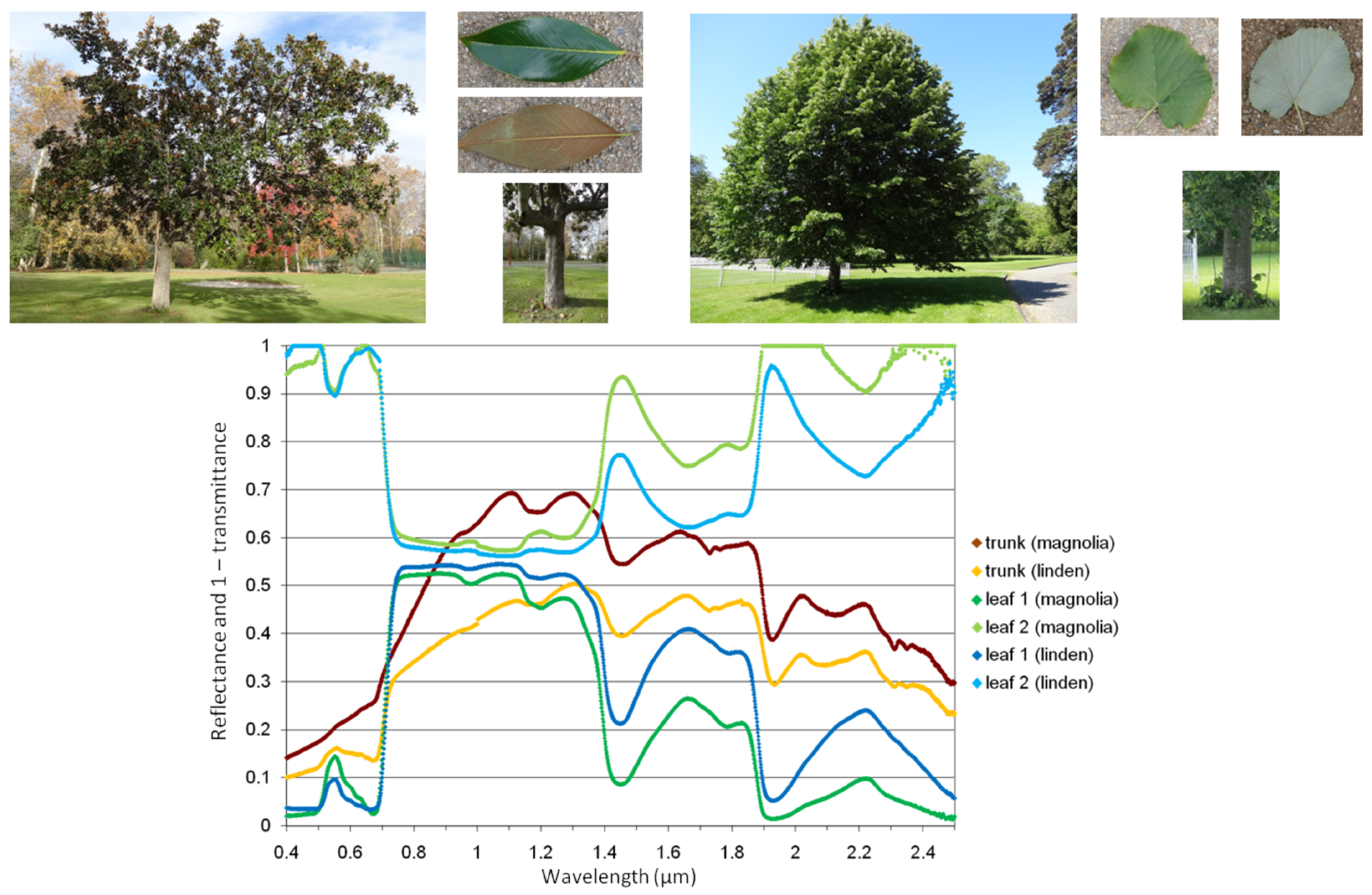
2.1. Study Site and Field Measurements

A field campaign was carried out during 4 days between 3and 13 June 2013, on the CREPS site located in Toulouse, southwest of France (Center of Resources, Expertise and Sportive Performance; 43°34′04.48″ N, 1°28′37.11″ E) [43]. It consisted in both geometric and optical characterization of two single deciduous broadleaf trees, a magnolia tree (Magnolia grandiflora; Figure 1) and a linden tree (Tilia cordata; Figure 1). They were selected because they are isolated, cast a large shadow on a well-tended lawn, and have two different foliar densities and tree crown morphology. The magnolia appears to have a low leaf density with a crown with no specific shape while the linden has a higher leaf density with a crown like an elliptic paraboloid. The measured variables of interest were the leaf optical properties (hereafter named LOP) and the crown NPV reflectance (NPV stands here for trunk and branches), the 3D architecture from TLS acquisitions with the separation of leaves and NPV, the trunk diameter defined by the diameter at breast height (DBH), the tree leaf area index (hereafter mentioned indifferently in this paper LAI or tree LAI), and the leaf angular properties, approximated by the average leaf angle (ALA) for an ellipsoidal leaf angle distribution (LAD).

For each tree on 13 June 2013, LOP were measured with a portable ASD FieldSpec^® 3 spectroradiometer (Analytical Spectral Devices Inc., Boulder, CO, USA) with the leaf-clip accessory. A set of 10 leaves taken at the half of the crown height and located randomly in the sunlit and the shade part of the crown were sampled. For two distinct positions on each leaf, 20 reflectance measurements were acquired and the same was performed by using the white and black panels in the leaf-clip to derive both leaf reflectance and transmittance following the protocol of [44]. Trunk reflectance was measured with the same spectroradiometer, and the contact probe accessory. Measurements were acquired on 10 different locations, where maximum contact with the trunk can be achieved, and avoiding the sunlight to interfere with the measure by placing a black tissue all around the contact probe. For each trunk location, 20 reflectance measurements were acquired, and calibration was performed by using an external Spectralon^® with known reflectance. Then, for both leaf and trunk measurements, common spectral discontinuities due to changes between the three optical fibers in the instrument over the 0.35–2.5 µm range were corrected by a parabolic correction included in the ViewSpec Pro software (Analytical Spectral Devices application). No smoothing was applied. At last, only the spectral average values of the derived optical properties are kept for the purposes of this study based on a simulation analysis (trunk reflectance was assigned to NPV reflectance including branches as well). They are plotted in Figure 1.

On the same day, on 13 June 2013, multiple acquisitions with a TLS instrument were performed in order to reconstruct the 3D shape of trees from the acquired point clouds. This LiDAR instrument has been developed by ONERA: GIBI (Gated Imager with Burst Illumination) [45]. It has multi-target capability and took several multi-angular acquisitions leading to point clouds with an angular step set to 1° between consecutive laser shots [45]. The data geo-referencing was performed based on known reference locations of French Geographic Institute (IGN) with centimetric accuracy. NPV can be separated from the leaves by combining reflectance information at 1.5 µm (LiDAR working wavelength and home-made calibration process), the shape and order of echo (first, intermediate, last). Trunk has a higher reflectance value at 1.5 µm than the LOP (Figure 1) and mainly present sharp and isolated LiDAR echoes while leaves usually have overlapping multiple ones. Single echoes highlight both NPV and leaves at the borders of the tree crown while intermediate echoes represent part of the signal transmitted through the tree and partially intercepted. Consequently, NPV were discriminated by manually thresholding the reflectance and extracting single echoes [46]. This step is manually completed inside the tree crown when the tree LAI is high like for the linden. Then, NPV and leaves were triangulated from the 3D point clouds by accounting for the specific leaf dimensions (e.g., 0.15 m for the magnolia and 0.08 m for the linden tree) with a processing algorithm. For the linden, 96% of the facets over a total of 836,543 represents leaves compared to wood elements while it is 87% over 784,684 for the magnolia. This process leads to building what is further called the 3D TLS-based tree models, from which tree height, crown projected area, and crown volume were estimated. The tree height is given by the highest cloud point acquired by the TLS instrument. The crown projected area is retrieved with an accuracy of 0.01 m² by triangulating the surface of a polyline defined by the projected 3D point cloud on a ground plane the furthest from the tree trunk position. The crown volume is estimated at an accuracy of 0.01 m³ by defining a convex envelope encompassing all cloud points within the crown. At last, DBH was measured in situ for the two trees at 1.3 m from the ground.

The tree LAI (i.e., the ratio between the total leaf area and the crown projected area at ground) was directly estimated thanks to the knowledge of the total area of the leaf triangles and the crown projected area, as previously computed from TLS data post-processing. It was retrieved at 1.28 m².m⁻² for the magnolia and 2.27 m².m⁻² for the linden tree. The ALA for each tree was estimated by importing the leaf triangles of the TLS-based tree models into the radiative transfer model DART, where they are converted into turbid voxels of dimensions 0.4 m × 0.4 m × 0.4 m. For each voxel, DART computes the mean orientation of the leaf triangles by sampling the ALA with a discrete number of angles between 0 and 90°. This number is arbitrary fixed to 10 to keep the computation time moderate. A mean ALA of 63 and 51° is retrieved, respectively, for the magnolia and the linden, with a similar standard error of 13°. Then, in order to assess the influence of the TLS-based reconstruction accuracy on the previous estimations of the tree LAI and the ALA, these values were further compared to estimations derived from two additional methods: an indirect calculation of LAI and ALA from optical measurements with a LAI-2000 plant canopy analyzer (LI-COR, Inc., Lincoln, NE, USA) and an allometric equation from [47] to estimate LAI. On one side, the comparison of ALA values derived from the TLS-based tree models and the LAI-2000 shows a good agreement with a difference of 2° for the linden and 7° for the magnolia. Their respective values are relatively close to 57.58°, which is the value corresponding to a spherical LAD [48] (later assumed in some 3D tree modeling scenarios). On the other side, the comparison of LAI values is much less straightforward and depends on the leaf clumping, and both the leaf and wood elements density. Complete details about the theory for the allometric equation, how the measurements were taken with the LAI-2000, and discussions in comparing the different results are described in Appendix A. At last, in the following sections of this study, only LAI and ALA values retrieved from TLS data are further used for the 3D tree modeling scenarios since the references are the TLS-based tree models.

2.2. General Methodology

The global methodology is structured as depicted in Figure 2. In Section 2.3, the DART canopy radiative transfer model is used to consider multiple 3D tree models, and simulates observations that will serve to extract the tree crown transmittance. First, in the Section 2.3.1, several strategies are defined to model the 3D structure of a single tree: a schematic and generalized representation with a fixed geometry named the empirical tree model (noted E) that lies as a compromise for the needs of atmospheric correction models [17] and more realistic representations that are derived from both TLS acquisitions and field measurements (models numbered from 1 to 6). Then, all these tree models are represented in 3D mockups into DART. These mockups are designed to represent the scene viewed by a pixel from the remote sensing image. The other inputs of DART are composed of fixed and variable parameters, which are set in the Section 2.3.2. For instance, some parameters are fixed by the tree geometry and the field measurements for the tree models from n°1 to 6. The, the simulations are run and stored in lookup tables (LUTs) where the outputs of interest are extracted, that are the irradiance fractions received at ground in the tree shadow. From these latter, the tree crown transmittance $T_c$ is computed as explained in the Section 2.3.3 and Appendix B. Next, the analysis of $T_c$ is split into two parts. The first part is dedicated to the building of a regression relationship aiming to predict $T_c$ from the empirical tree model. To this end, a preliminary sensitive analysis is carried out in order to select the most important factors to build the regression. The theory is detailed in Section 2.4 and the results in Section 3.1. The second part is based on the comparison between the tree models; more precisely, predicted $T_c$ from the empirical one and simulated $T_c$ from the more realistic models. The metrics of comparison are stated in Section 2.5. The goal is to have a better understanding of the sources of errors in estimating $T_c$ due to (i) a degradation in the tree model abstraction from a realistic case relying on in situ measurements (tree models from n°1 to 6) and (ii) the strong assumptions made by summarizing each tree by a fixed geometry for the sake of generalization (tree model E compared to those from n°1 to 6). In Section 3.2, results are further shown depending on their spatial and spectral variability and their dependence to some variable parameters defined as inputs to DART simulations. At last, surface reflectance retrieval performances are analyzed following the 3D tree models in Section 3.3, based on the metrics defined in Section 2.6 linking $T_c$ and reflectance computation in the tree shadow.

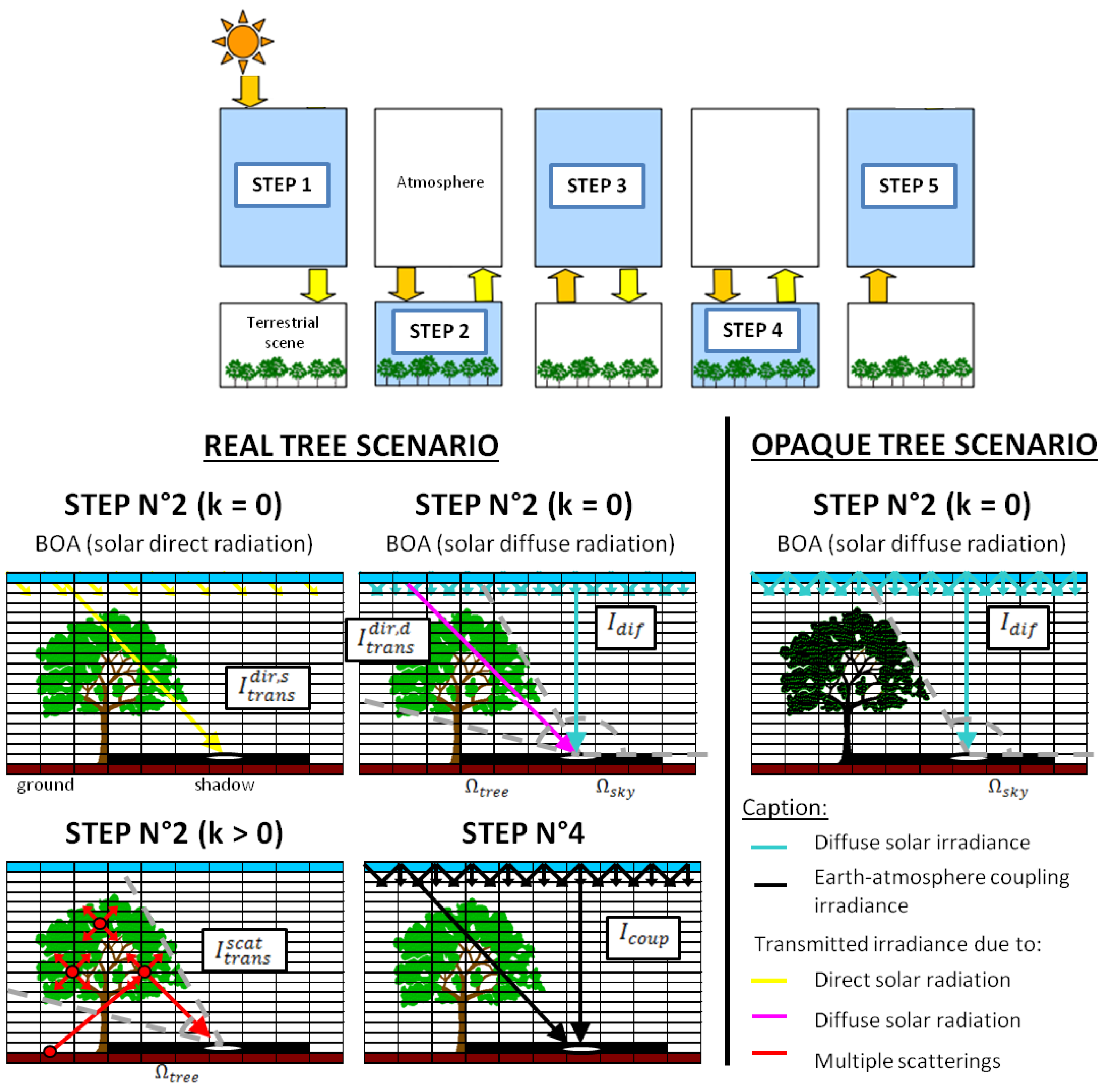
2.3. DART Canopy Radiative Transfer Model: Tree Modeling, Simulation Setting, and Transmittance Extraction

DART is a radiative transfer model in the Earth surfaces and the atmosphere, developed since 1992 in CESBIO (cesbio.cnrs.fr) and patented in 2003. Toulouse III University provides free licenses for research and education (dart.omp.eu). DART relies on an adaption of the so-called discrete ordinate method where radiation is tracked along a finite number of directions within any 3D urban/natural landscapes for any experimental/instrument configuration (atmosphere, topography,...) across the optical spectral domain (from ultraviolet to thermal infrared). It provides two major types of results:

• Remote sensing observations: satellite, aircraft, and ground imaging spectroradiometers and scanning LiDAR (discrete return, waveform, photon counting, TLS) systems.
• Radiative budget: 3D, 2D, and 1D distributions of absorbed, emitted, scattered, and intercepted radiation, including the solar-induced chlorophyll fluorescence signal of 3D vegetation.

DART is continuously improved. For example, its radiative coupling of the atmosphere and Earth surfaces with topography [49], and its atmospheric thermal infrared modeling [50] were recently improved. The major ongoing improvement deals with the introduction of bi-directional Monte Carlo methods that further improve its accuracy and potential to simulate large landscapes through the reduction of simulation time and needed computer memory [51].

DART uses specific input parameters for the optical properties and the geometry of the scene it simulates, the illumination and viewing conditions, and the sensor characteristics. It is very suited to assess different modeling strategies, especially for the tree architecture. More detail on the DART model is given in [35,52].

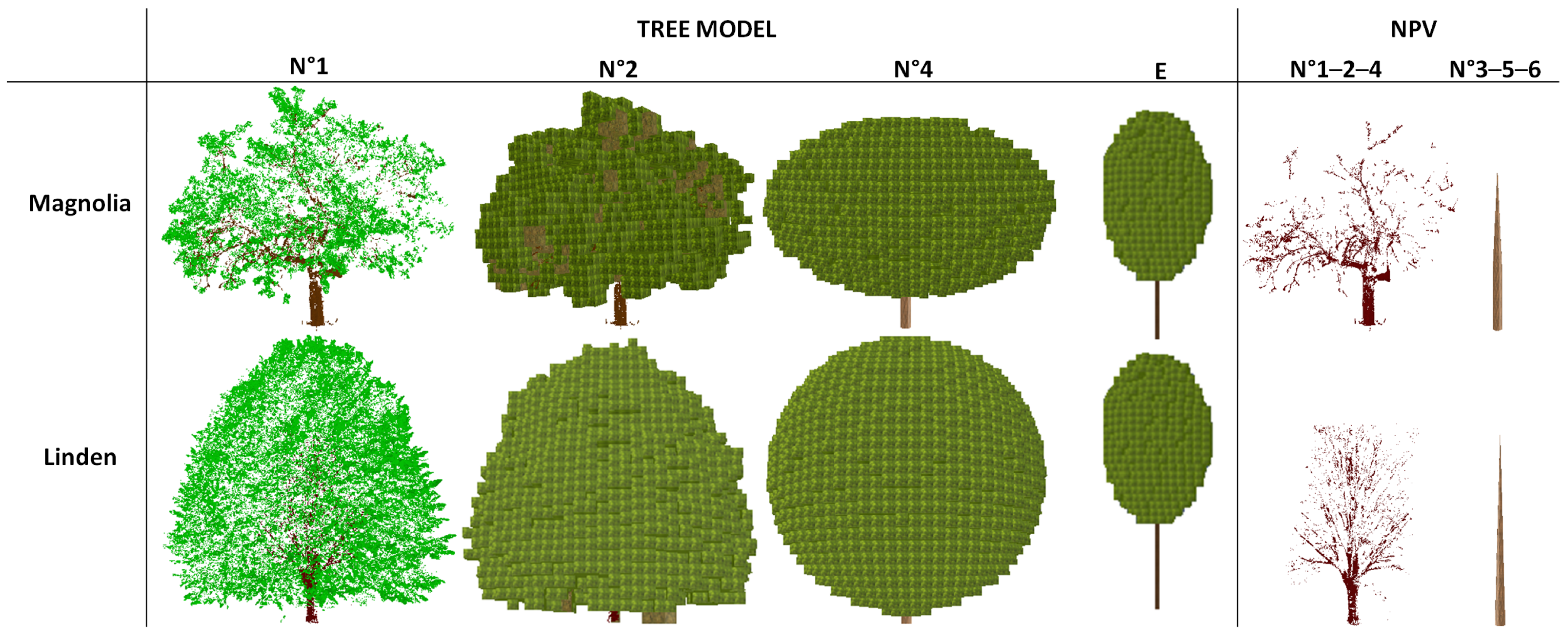
2.3.1. 3D Tree Modeling Scenarios

On the one hand, a very simplified tree model based on a geometric voxel-grid representation is considered. It originally refers to the “reference tree model” defined in [17] in order to bring a general correction baseline adapted to urban areas for atmospheric correction in the tree shadows. Its dimensions are arbitrarily fixed following mean statistics of urban single trees and allometric equations. The tree crown is ellipsoidal, which is an assumption often used in the literature [53,54]. There are no branches and the trunk is cylindrical outside the crown and conical inside it (Figure 3,

Table 1. Geometric configuration for each abstract tree model numbered from n°1 to 6 based on the TLS measurements (magnolia / linden) and for the empirical tree model E.

Tree Model	1	2	3	4	5	6	E
	(TLS-Based)	(Discrete Voxel-Grid)	(Discrete Voxel-Grid)	(Geometric Voxel-Grid)	(Geometric Voxel-Grid)	(Geometric Voxel-Grid)	(Geometric Voxel-Grid)
Leaves (L), trunk (T) and branches (B) modeling	Triangles (L+T+B)	Turbid voxels (L) and triangles (T+B)	Turbid voxels (L) and geometric (T), no branch	Turbid voxels (L) and triangles (T+B)	Turbid voxels (L) and geometric (T), no branch	Turbid voxels (L) and geometric (T), no branch	Turbid voxels (L) and geometric (T), no branch
Tree height [m]	9.48/11.56	9.48/11.56	9.48/11.56	9.65/11.90	9.65/11.90	9.65/11.90	14.2
Crown ellipsoid dimensions in x, y, z [m x m x m]	-	-	-	13.47 × 11.81 × 8.45 / 11.40 × 11.94 × 11.4	13.47 × 11.81 × 8.45 / 11.40 × 11.94 × 11.4	13.47 × 11.81 × 8.45 / 11.40 × 11.94 × 11.4	6 × 6 × 9.4
Trunk cylinder height below & inside crown [m]	-	-	1.2 & 6.34/0.5 & 8.55	-	1.2 & 6.34/0.5 & 8.55	1.2 & 6.34/0.5 & 8.55	4.8 & 7.2
DBH [m]	-	-	0.5/0.42	-	0.5/0.42	0.5/0.42	0.4
Crown projected area [m2]	117/119	98/97	98/97	125/107	125/107	125/107	28
Crown volume [m3]	339/669	280/581	280/581	704/812	704/812	281/579	177

and

Table 2. Variable parameters (their acronyms are highlighted in italics and bold) used for the empirical tree model E and their respective fixed values for the abstract tree models from n°1 to 6 based on TLS measurements (magnolia / linden).

Tree Model	1	2	3	4	5	6	E
	(TLS-Based)	(Discrete Voxel-Grid)	(Discrete Voxel-Grid)	(Geometric Voxel-Grid)	(Geometric Voxel-Grid)	(Geometric Voxel-Grid)	(Geometric Voxel-Grid)
Tree LAI [m2.m−2]	TLS-fixed	TLS-fixed	TLS-fixed	(1.28/2.27) 1	(1.28/2.27) 1	(1.28/2.27) 1	0.5–1–1.5–2–2.5–3–3.5–4–6–8
LAD (distribution: ALA [°])	TLS-fixed	Computed (ellipsoidal: 63 / 51)	Computed (ellipsoidal: 63 / 51)	Simplified (spherical) 2	Simplified (spherical) 2	Simplified (spherical) 2	Simplified (ellipsoidal: 30–57.58–70)
Leaf clumping or POROSITY [%]	TLS-fixed	Computed	Computed	Absent	Absent	Random distribution 3: 28.5 / 60	Random distribution: 0–30–70

¹ fixed from the direct calculation based on the TLS measurements; ² spherical LAD has no ALA; ³ percentage of gaps for a horizontal random distribution in the tree crown.

). This empirical tree model, noted tree model E, aims at giving first insights about the general behavior of $T_c$.

On the other hand, there is a need to compare this simplified empirical tree model with realistic scenarios. The most realistic tree representations are assumed to come directly from the TLS measurements described in Section 2.1, noted tree model n°1 (Figure 3, Table 1 and Table 2). Then, several abstract versions are derived from these TLS-based tree models and chosen in part following the work of [30]. They are categorized as discrete and geometric voxel-grid representations: they are based on the tree crown shape, leaf distribution, orientation and clumping, and the presence or absence of NPV. Discrete voxel-grid representations, noted in tree models n°2 and 3, come from the conversion of the leaf triangles of tree model n°1 into turbid voxels, preserving the global shape of the tree crown and the tree LAI but leading to a coarser modeling of leaf clumping within the crown and an approximate LAD depending on the voxel size (Figure 3). Geometric voxel-grid representations, noted in tree models n°4–6, consider the simplification of the tree crown shape with turbid ellipsoids whose dimensions is chosen to fit as much as possible the maximum spatial extents of those of discrete tree models. As such, these geometric models get closer to the tree model E except that the tree global dimensions differ. Then, compared to tree models n°2 and 3, tree LAI is the same and the LAD is assumed to be spherical (LAD type commonly chosen in the literature when unknown). Leaves are uniformly distributed, assuming that there is no clumping, except for tree model n°6, which has a POROSITY representing a percentage of gaps within the tree crown [55]. Actually, POROSITY simulates leaf clumping (assumed to be a proxy for it) in order to better reproduce the total leaf volume from discrete to geometric tree models for a same LAI vertical distribution. It is computed as the ratio of the number of voxels full of leaves between the geometric and the discrete tree models. At last, tree models n°1, 2, and 4 have a TLS-based NPV representation (trunk and branches) while tree models n°3, 5, and 6 have a simplified one, the same as tree model E (Figure 3).

2.3.2. Definition of the Fixed and Variable Parameters for Simulation Purposes

Two sets of variable parameters are defined to be used with DART: seven parameters (LAI, ALA, POROSITY, LOP, SZA, VISI, BACKGROUND) for the tree model E following the work of [17] and two parameters (SZA, BACKGROUND) for the tree models from n°1 to 6. Then, globally, Table 2 and

Table 3. DART geometric configuration of the scene, sun direction, atmosphere, and sensor (the acronyms of the variable parameters are highlighted in italics and bold).

	Variable [Units]	Values
Sun geometry	Zenith angle [°] (SZA)	30–45–60
	Azimuth angle [°]	90 (relative value)
Sensor geometry	Zenith /Azimuth angles [°]	0 / 0
Spectral bands	Number 1 / range [µm]	138 / 0.4–2.5
	FWHM 2 [nm]	Vis–NIR: 3.7 & SWIR: 6
Atmospheric conditions	Gaseous atmospheric profile	Mid-latitude summer
	Aerosol type	Urban
	Visibility [km](VISI)	Tree model n°1–6: 23 Tree model E: 10–23
Scene	Dimensions in x, y, z [m × m × m]	Tree model n°1–6: Magnolia: 20 × 30 × 10 Linden: 20 × 30 × 12 Tree model E: - SZA < 60°: 22.8 × 22.8 × 14.0 - SZA = 60°: 30.8 × 30.8 × 14.0
	Voxel size in x, y, z [m × m × m]	0.4 × 0.4 × 0.4

¹ bands inside atmospheric water vapor windows and with low signal-to-noise ratio are removed; ² full width at half maximum.

and Figure 4 give the values of the variable and fixed parameters. For tree models from n°1 to 6, optical properties, namely LOP and NPV reflectance, are fixed to the field measurements (Figure 1). For the tree model E, LOP are those of three tree species from the spectral database ANGERS03 [56]: Quercus palustris, Populus alba, and Liquidambar styraciflua (Figure 4). They were selected because they have respectively the highest leaf transmittance, the highest leaf reflectance and average leaf reflectance and transmittance [17]. Trunk reflectance is “deciduous bark” from the DART spectral database. The scene has dimensions such that it includes the tree model and its cast shadow. Its voxel size (0.4 m) is adapted to the scene element dimensions. The BACKGROUND reflectance is either “rye grass” or “dark asphalt” from the DART spectral database (Figure 4). The atmosphere is typical of urban environments with either a standard urban visibility (VISI = 5 km) or clear sky conditions (VISI = 23 km). The solar zenith angle is defined for three hours of the day (SZA = 30/45/60°). The spectral range is 0.4–2.5 µm with a sampling and spectral resolution typical of visible and near infrared (Vis–NIR) and shortwave infrared (SWIR) HySpex sensors (Norsk Elektro Optikk). Finally, a total of 3240 $T_c$ observations are simulated for the first set of variable parameters and 6 $T_c$ observations per tree model for the second one.

2.3.3. Tree Crown Transmittance Derived from Radiative Transfer Budget in the Tree Shadow

The irradiance $I_{tot}$ of any ground point in the tree shadow corresponds to the TOC solar direct and diffuse irradiance $I_{TOC}$ that has interacted or not with the tree crown materials (e.g., leaves and NPV). Here, $I_{tot}$ is assumed to be the sum of three terms: the tree crown transmitted irradiance $I_{trans}$, the atmospheric diffuse solar irradiance $I_{dif}$ that directly illuminates the ground, and the earth–atmosphere coupling irradiance, $I_{coup}$. The irradiance due to the scattering by the surrounding environment is neglected since a single isolated tree in a flat scene is considered. $I_{trans}$ can be split into three components: $I_{trans}$=$I_{trans}^{dir,s}$+$I{ }_{trans}^{dir,d}$+$I_{trans}^{scat}$, with $I_{trans}^{dir,s}$ and $I{ }_{trans}^{dir,d}$ due to the direct transmission through the tree crown of the direct sun and diffuse atmosphere radiation, respectively, and $I_{trans}^{scat}$ due to the tree crown transmitted radiation that has been scattered at least once by the tree, and possibly also with the ground. These components are retrieved from DART as explained in Appendix B. Some of them are used to compute $T_c$ and are extracted for each ground voxel located in a mask manually drawn over the tree shadow. For the three SZA, this mask includes a number of 162, 250, and 396 voxels for the tree model E, 590/530, 720/600, and 910/800 voxels for tree models from n°1 to 3 for linden/magnolia, and 630/630, 790/730, and 1,160/910 voxels for those from n°4 to 6 for linden/magnolia. Then, $T_c$ is expressed as a percentage as follows:

$$T_c=\frac{I_{trans}}{I_{TOC}}\times 100=\frac{\left(I_{trans}^{dir,s}+I_{trans}^{dir,d}+I_{trans}^{scat}\right)}{I_{TOC}}\times 100=\left(T_{dir}+T_{scat}\right)\times 100$$

(1)

with $T_{dir}$ for direct transmission, and $T_{scat}$ for transmission with multiple scattering.

2.4. Statistical Regression for the Empirical Tree Model

With the empirical tree model E, the objective is to establish a statistical regression to predict the mean of $T_c$ in the tree shadow. The methodology is taken from [17] and summarized thereafter. The regression equation is determined by the averaged $T_c$ over the tree shadow mask for the 3240 DART-simulated observations.

A first step consists in reducing the number of explanatory input parameters in the regression equation based on a variance analysis (ANOVA) and the computation of a sensitive index η². This index is the ratio of the sum of squares values accounting for the single and combined effects of the input parameters on the variance of $T_c$ over the total sum of square values [57,58]. First, the input parameters and the output $T_c$ are conditioned to vary linearly within their range, normalized and centered. Then, a second order polynomial expression with the first order interactions between the inputs and the output is built. The goodness of fit of this expression is assessed with the root mean square error (RMSE), the adjusted coefficient of regression ($R_{adj}^2$), and the metric of statistical significance (p-value). At last, η² is computed for each input parameter and each of the 138 spectral bands. A spectral analysis is performed over four LAI ranges: full (0.5 m².m⁻² ≤ LAI ≤ 8 m².m⁻²), low (0.5 m².m⁻² ≤ LAI ≤ 2 m².m⁻²), medium (2 m².m⁻² ≤ LAI ≤ 3.5 m².m⁻²), and high range (3.5 m².m⁻² ≤ LAI ≤ 8 m².m⁻²). Finally, the most influent parameters are selected among the highest η² values.

A second step aims at building a multivariate linear regression equation from this reduced number of input parameters. A stepwise strategy is chosen from a second order polynomial expression with first order interactions in order to decrease the number of terms in the final equation [59]. The following equation is finally determined:

$$\begin{array}{r}Y\left(\lambda \right)=a_0\left(\lambda \right)+a_1\left(\lambda \right)\times X^{\prime }+a_2\left(\lambda \right)\times X^{″}+a_3\left(\lambda \right)\times {X^{\prime }}^2+a_4\left(\lambda \right)\times {X^{″}}^2+a_5\left(\lambda \right)\times {X^{\prime }}^3\\ +a_6\left(\lambda \right)\times {X^{\prime }}^4+a_7\left(\lambda \right)\times X^{\prime }\times X^{″}+a_8\left(\lambda \right)\times X^{\prime }\times {X^{″}}^2\end{array}$$

(2)

with $\left\{\begin{array}{l}Y=\mathit{log}(T_c+1)\\ X^{\prime }=e^{-0.5\times LAI}\\ X^{″}=\mathit{cos}(SZA)\end{array}\right.$, λ the spectral band and $a_{\mathrm{1..8}}$ the eight regression coefficients.

The regression coefficients are bootstrapped over 1000 repetitions and their mean values are attributed to the Equation (2). Performance will be assessed with RMSE and R² over all the 3240 $T_c$ observations.

2.5. Metrics to Compare Tree Crown Transmittances

The analysis to compare $T_c$ between TLS-based, discrete/geometric voxel-grid and empirical tree models is split into two parts: a spectral analysis carried out on $T_c$ averaged over the tree shadow and a spatial analysis taking into account its variability computed at shadow. A base simulation scenario is assumed to be with SZA = 45° and BACKGROUND = grass for TLS-based, discrete, and geometric voxel-grid tree models, and LAI = 3 m².m⁻², LOP = quercus, ALA = 57°, POROSITY = 0%, SZA = 45°, VISI = 23 km, and BACKGROUND = asphalt for the empirical one.

For the spectral analysis, the objective is to assess the mean spectral bias error (B) in simulating and predicting $T_c$ with different levels of 3D simplification of the tree compared to a reference case. This reference will be assumed to be first the TLS-based tree model and then the empirical one for 6 $T_c$ observations. Afterwards, the sign of B will show if the compared tree model overestimates (B < 0) or underestimates (B > 0) $T_c$ compared to the two reference tree models. B is expressed in percentage and computed as follows:

$$B_{ref,m,k}={\displaystyle \sum }_{i=1}^N\frac{\left(T_c^{ref}\left({\lambda }_i\right)-T_c^m\left({\lambda }_i\right)\right)}{N}\times 100$$

(3)

with N the number of spectral bands (λ the wavelength), ref the reference tree model, m the compared tree model, and k one DART $T_c$ observation.

For the spatial analysis, the objectives are to have a better physical understanding of radiation interception mechanisms within a scene with an isolated tree, and to quantitatively assess $T_c$ spatial heterogeneity when computed at tree shadow. To achieve this, the fraction of intercepted radiation will be observed along the tree elevation profile [60], and the distribution variability of $T_c$ in the tree shadow will be studied through the calculation of a measure of statistical dispersion, namely the interquartile range ($IQR=Q_3-Q_1$ with $Q_1$ and $Q_3$ being the first and third quartile of a boxplot representation). These analyses will be examined by separating the contribution of $T_{dir}$ and $T_{scat}$ from $T_c$. This spatial study is performed for the base simulation scenario at the wavelength 0.8 µm, for which the contribution of $T_{scat}$ is close to its maximum value.

2.6. Metrics to Assess Surface Reflectance Retrieval Performance

Following the previous spectral analysis, the next step is to evaluate if the simulated and predicted $T_c$ from the different tree models fit the requirements to retrieve surface reflectance correctly in a tree shadow. This relies on the fact that all sources of errors on the estimation of the radiative components are null except those associated to $T_c$. As such, the desired accuracy in reflectance retrieval is fixed according to two atmospheric correction models able to achieve an exact calculation of the 3D radiative terms to retrieve surface reflectance at high spatial resolution: ATCOR-4 [12] and ICARE [15]. Assuming a flat terrain and avoiding the specular and backscattering regions, ATCOR-4 performance demonstrated an absolute error of 0.02 and 0.04 for an initial reflectance below 0.10 and above 0.40 respectively, and good agreement with field data in the range 0.01–0.03. ICARE showed a maximum peak to peak accuracy of 0.04 in the retrieved reflectance compared with field data for some spectral bands and pixels located in shadows cast by buildings. Based on the performances and accuracies of these models already stated in the Introduction, three absolute reflectance levels of error are accordingly defined as good performances (error < 0.02), acceptable performances (0.02 ≤ error ≤ 0.03), critical performances (0.03 < error ≤ 0.04), and unacceptable performances (error > 0.04).

A first goal aims at evaluating the global mean spectral error determined by fixing thresholds $S_{NB}$ on the computation of the normalized mean bias (NB) compared to $T_c$ for the reference tree model. As previously in Section 2.5, the reference will be assumed to be first the TLS-based tree models and then the empirical one for 6 $T_c$ observations. Then, NB and $S_{NB}$ are expressed in percentage and computed as follows:

$$N{B}_{ref,m,k}={\displaystyle \sum }_{i=1}^N\frac{\left|T_c^{ref}\left({\lambda }_i\right)-T_c^m\left({\lambda }_i\right)\right|}{N}\times 100$$

(4)

$$S_{NB}=\frac{\Delta T_c}{T_c}=\frac{\Delta \rho }{\rho }\times \frac{I_{tot}}{I_{trans}}\times 100$$

(5)

with ρ the ground reflectance and the absolute reflectance and Δρ error.

A second goal is to assess this same error when neglecting either $T_{dir}$ or $T_{scat}$ at two specific spectral bands, 0.67 and 0.8 µm (the red and NIR band commonly used for vegetation indices calculation), where the contribution of $T_{scat}$ greatly differs. This time, the only reference tree model will be the TLS-based ones (the more realistic scenario) and the base simulation observation is still SZA = 45° and BACKGROUND = grass. The same three absolute reflectance errors are considered with the same evaluation of achieved good/acceptable/critical/unacceptable performances for atmospheric correction purposes.

Thus, for both these two goals, $S_{NB}$ will be calculated with the ratio $I_{tot}/I_{trans}$ determined through the analysis of the radiative transfer budget in the tree shadow separately for the linden and the magnolia tree. For the first goal, the reflectance of two soil types, namely asphalt and grass, are considered (cf. Figure 4). Their mean spectral reflectance over 0.4–2.5 µm is fixed to 0.08 and 0.18, respectively. For the second goal, only grass is considered. Its reflectance in the red and NIR is equal to 0.045 and 0.484, respectively.

3. Results

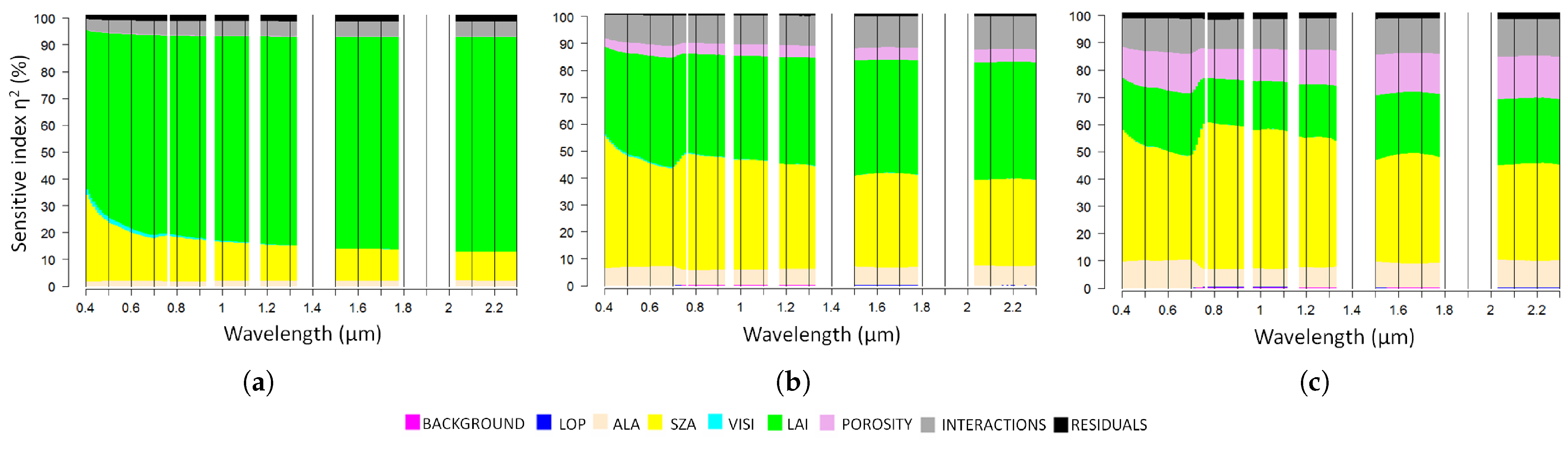
3.1. Tree Crown Transmittance for the Empirical Tree Model: Sensitivity Analysis, Regression Building, and Prediction

Concerning the determination of the most influent input parameters to predict $T_c$, the adequacy of the fitting equation during the sensitive analysis gives mean RMSE values of 5.6%, 3.4%, 0.8%, and 0.5% and mean $R_{\mathit{adj}}^2$ values of 0.98, 0.98, 0.99, and 0.98, respectively for the full, low, medium, and high LAI ranges, with mean p-values below 1% for all of them (very low spectral variability of RMSE, $R_{\mathit{adj}}^2$, and p-values over 0.4–2.5 µm). The analysis of the sensitive index η² results highlights the predominance of two parameters: SZA and LAI (Figure 5). LOP, BACKGROUND, and VISI are negligible. The two first are barely influent in the NIR–SWIR for the high LAI range while the third represents at maximum 2% for the low LAI range in the visible (e.g., aerosol atmospheric diffusion). For the low LAI range, the LAI contribution accounts for between 58% and 79%, SZA between 11% and 32%, and the interactions less than 5% for mainly ALA:SZA and, to a lesser extent, LAI:SZA (Figure 5a). From the medium to the high LAI range, the LAI predominance decreases and now ranges between 16% to 24%, to the benefit of SZA having an increased contribution between 34% and 53% (Figure 4c and Figure 5b). The interactions increase more than 10% and are dominated by ALA:SZA. The more LAI decreases, the more the impact of other parameters such as ALA and POROSITY grows, achieving a maximal contribution of 10% and 15% respectively.

A detailed analysis of the spectral variations of $T_c$ over 0.4–2.5 µm following the dominant parameter LAI is showed in Figure 6. For low LAIs, they monotonically increase and then start to saturate in the SWIR with an important variability following the input parameter variations. For LAI equal to 1 m².m⁻², the magnitude of $T_c$ varies between 15% and 65% with a single band maximum $T_c$ variation of 30% (Figure 6a). From low to high LAIs, $T_c$ rapidly decreases and achieves at maximum 18% for LAI equal to 3 m².m⁻², while becoming almost negligible for LAI equal to 6 m².m⁻² due to LAI saturation (Figure 6b,c). A barely visible spectral signature appears in the red-edge, NIR, and SWIR, highlighting the low influence of optical parameters such as LOP. The single band maximum T_c variation is of the order of 15% and 8.5%, respectively, for LAI equal to 3 m².m⁻² and 6 m².m⁻². Consequently, the study has being further limited to observations where LAI ≤ 4 m².m⁻², such that for higher LAI values, the tree crown is considered opaque to the transmission of incident radiation.

For the prediction of $T_c$, the performance over the 2592 $T_c$ observations for LAI ≤ 4 m².m⁻² gives mean R² higher than 0.9 and RMSE lower than 5%. After the bootstrap, the confidence interval of the performance ranges between 0.91 and 0.94 for R², and between 3% and 4.3% for RMSE. Comparing predicted and simulated $T_c$ for the empirical tree model shows a slightly skewed dispersion that is not wavelength-dependent, with an absolute maximum bias lower or equal to 10% (Figure 7).

3.2. Comparison of Tree Crown Transmittances from the Tree Modeling Scenarios

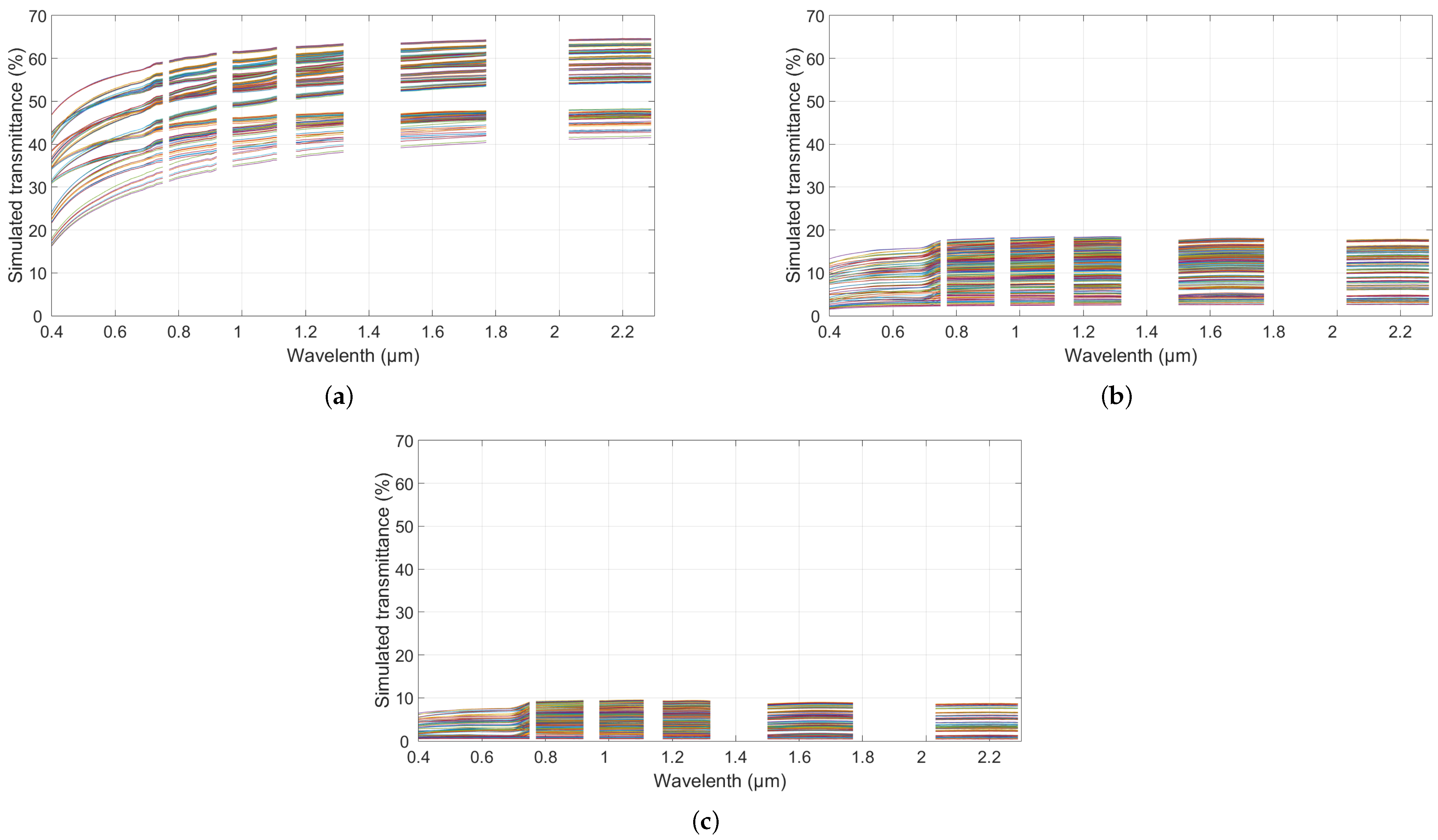
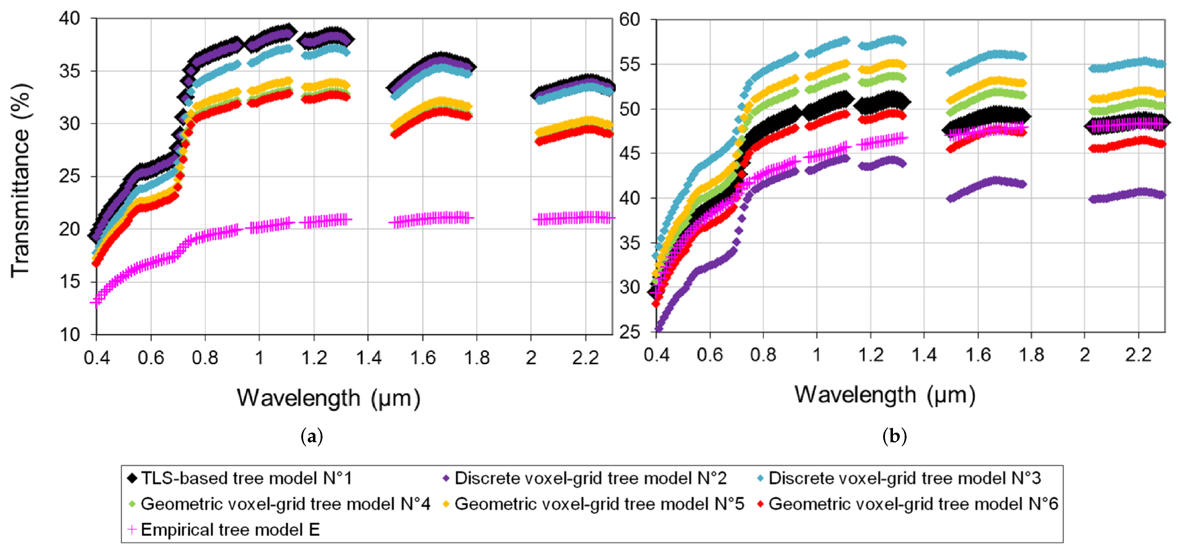
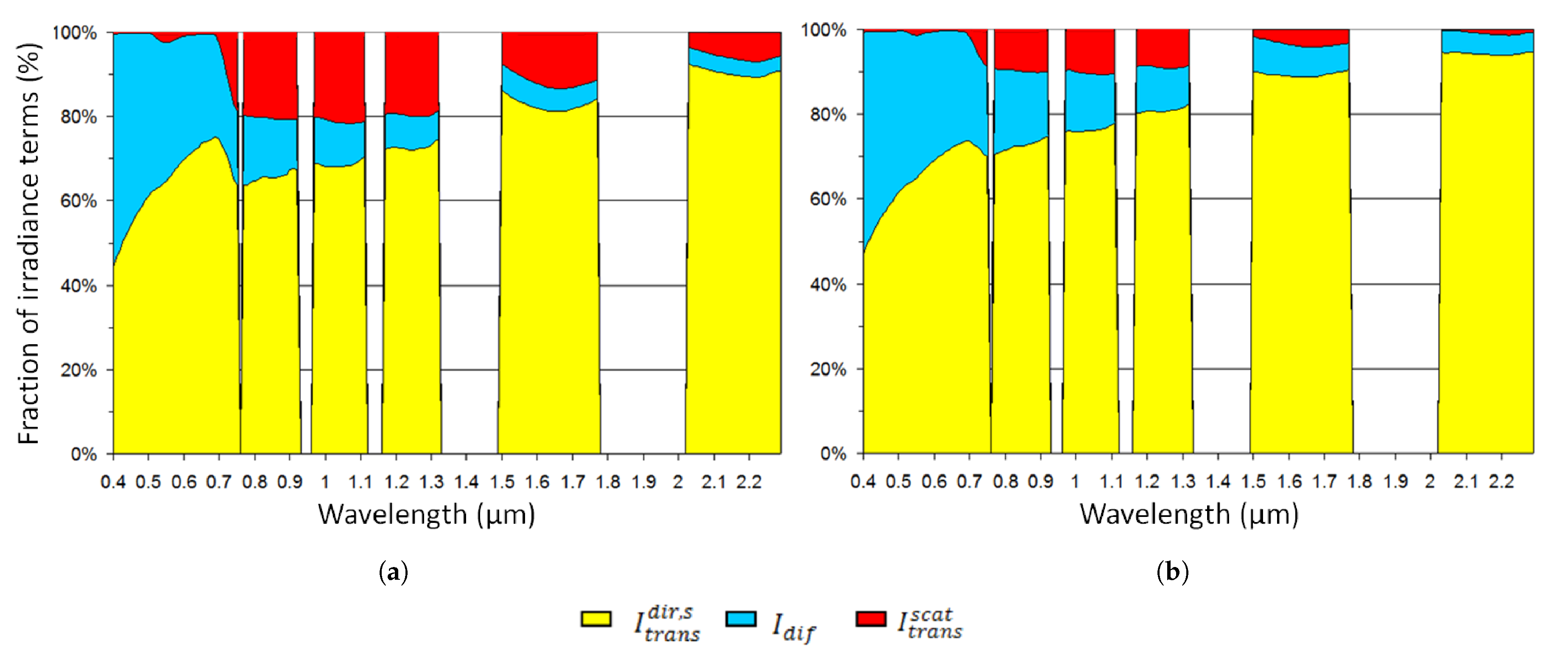
3.2.1. Spectral Analysis

On one side, the reference will be the TLS-based tree model n°1 compared to its derived tree simplified models from n°2 to 6. Results show that B ranges between −1.6% and 7.5% for the linden and between −6.4% and 8.2% for the magnolia tree (

Table 4. Comparison of the mean spectral bias error B expressed in % between the two reference tree models and different geometric tree representations (first column: T stands for the number of the compared tree models) for 6 $T_c$ observations (SZA = 30/45/60° and BACKGROUND = A – asphalt / G – grass) and the two tree species.

	Reference: TLS-Based Tree Model n°1
	Linden						Magnolia
T	30°/A	30°/G	45°/A	45°/G	60°/A	60°/G	30°/A	30°/G	45°/A	45°/G	60°/A	60°/G
2	0	0	0.1	0.1	0	0	6	5.9	7	6.9	8.2	8.1
3	0.9	1	1.1	1.2	−1.5	−1.6	−5.2	−5.2	−6.3	−6.2	−6.4	−6.4
4	7.4	7.5	4.5	4.6	4.4	4.6	3.1	3	1.8	1.8	1.7	1.7
5	7.1	7.1	4.3	4.4	3.6	3.7	−0.7	−0.8	−2.1	−2.1	−1.8	−1.8
6	6.3	6.4	3.6	3.7	3.6	3.7	−2.2	−2.2	−3.5	−3.4	−3	−3
	Reference: Empirical Tree Model E
	Linden						Magnolia
T	30°/A	30°/G	45°/A	45°/G	60°/A	60°/G	30°/A	30°/G	45°/A	45°/G	60°/A	60°/G
1	17.7	19	12.6	13.6	24.6	25.2	9.5	10.3	1.6	2.3	14.2	14.6
4	10.6	11.8	8.3	9.2	21	21.5	10.2	11.1	3.7	4.4	16	16.4

). For the base simulation scenario, $T_c$ between tree models seems to present a constant spectral shift, either positive or negative over 0.4–2.5 µm, and the calculation of the correlation coefficient shows values higher than 0.99 (Figure 8). Globally, the BACKGROUND impact is minor whatever the tree species and the tree model (B differences ≤ 0.2%). Then, for the linden tree, the discrete voxel-grid tree models show a good adequacy with the TLS-based tree model whatever the SZA value: absolute B errors are almost null for tree model n°2 and lower than 1.6% for n°3 (with a decrease in NPV proportion). A change occurs with geometric voxel-grid tree models with absolute B errors between 3.6% and 7.5%. Tree models n°4 and 5 behave the same and a very slight improvement is observed for tree model n°6 only at low SZA values. Globally, the errors in $T_c$ simulations tend to increase with low SZA values and B values are mainly positive leading to $T_c$ underestimations. For the magnolia tree and the discrete voxel-grid tree models, n°2 underestimates $T_c$ whereas n°3 overestimates it. These errors slightly increase with the increase in SZA values. On the opposite, the geometric voxel-grid tree models have lower errors with absolute B between 0.7% and 3.5% that seem less dependent of SZA variations. Tree model n°4 underestimates $T_c$ while n°5 and 6 overestimate it; this is in agreement with the trends observed for tree models n°2 and 3, respectively, the only difference being the type of NPV modeling.

On another side, the reference will be the empirical tree model E with its predicted $T_c$ for LAI equal to 1.28 m².m⁻² for the magnolia and 2.27 m².m⁻² for the linden tree and the three SZA values. Tree model E will be compared to the previous reference tree model n°1 and the tree model n°4, the latter being the closest in terms of geometry representation among tree models from n°1 to 6. The $T_c$ predictions show much more important bias whatever the tree model (B between 1.6% and 25.2%) than between the tree models n°1 and 4 (B between 1.7% and 7.5%) (Table 4). All B values are positive proving a systematic $T_c$ underestimation. The BACKGROUND impact is negligible. For the base simulation scenario, observing spectral variations of predicted $T_c$ demonstrates that for the linden tree there is a bias in $T_c$ magnitude which is spectrally dependent. This bias increases in the NIR and SWIR regions since the spectral shape of $T_c$ is no longer preserved (Figure 8a). For the magnolia tree, it appears that the global magnitude of $T_c$ fits in the average the one of the tree model n°1. However, the spectral variations of $T_c$ in the NIR and SWIR are also not preserved, but to a lesser extent (Figure 8b).

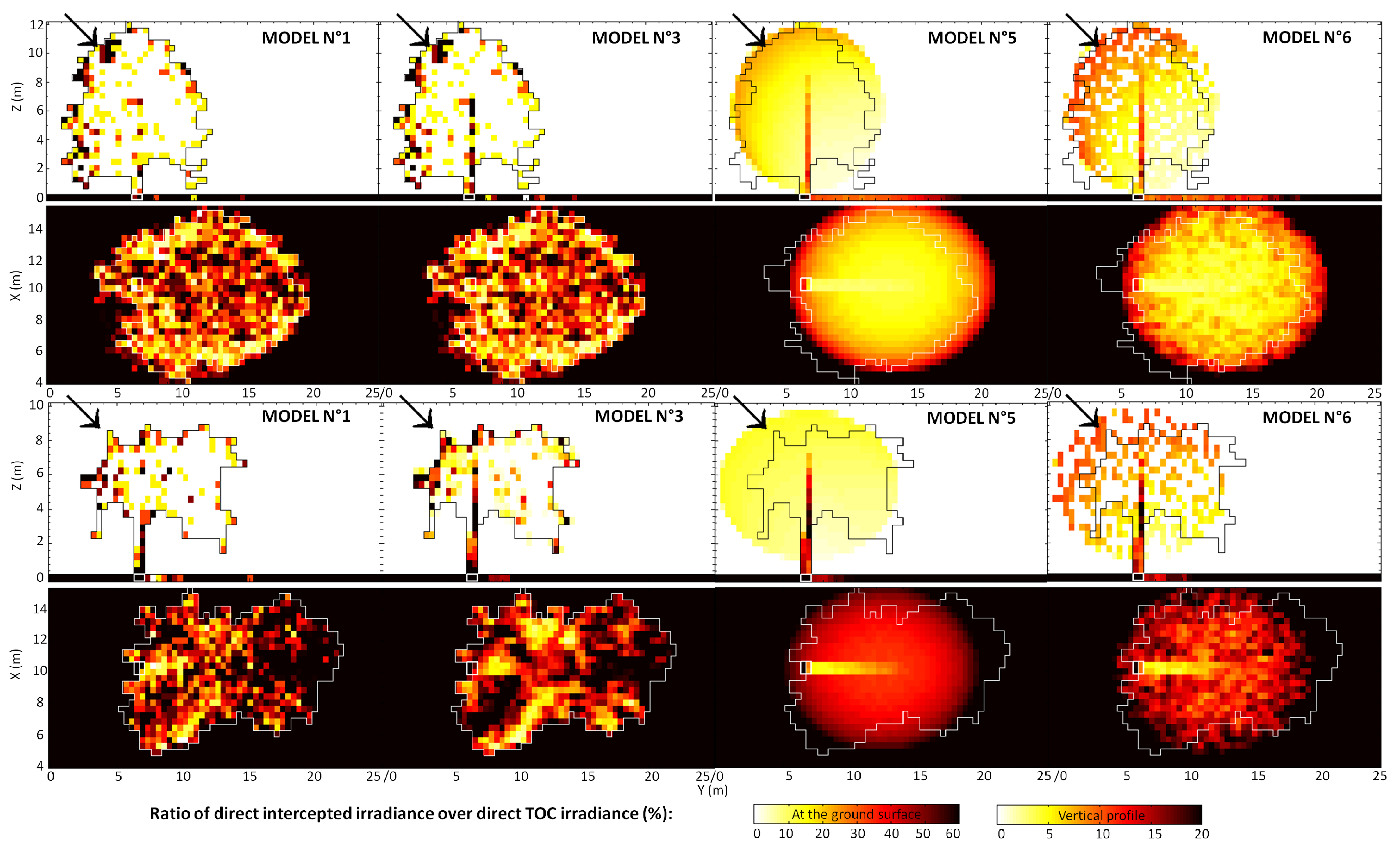
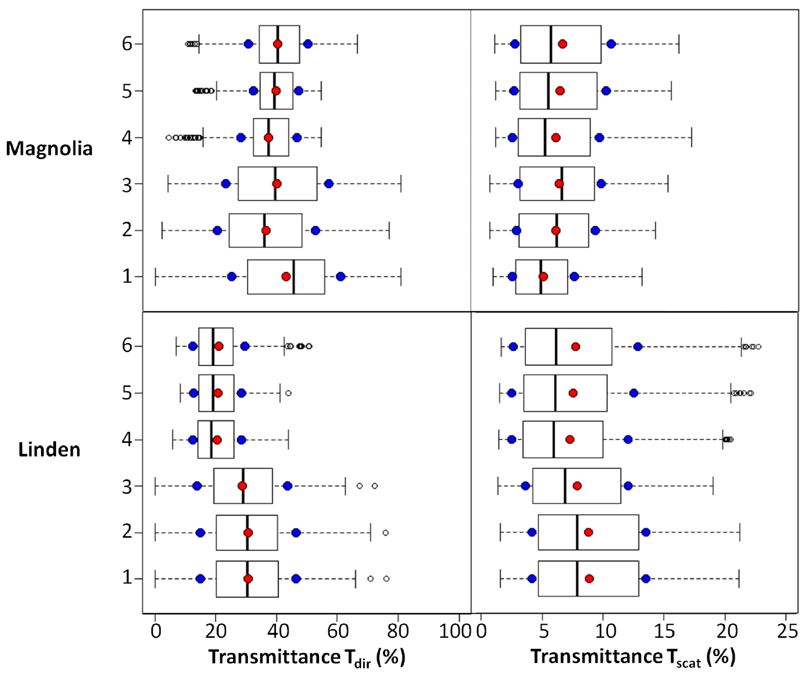
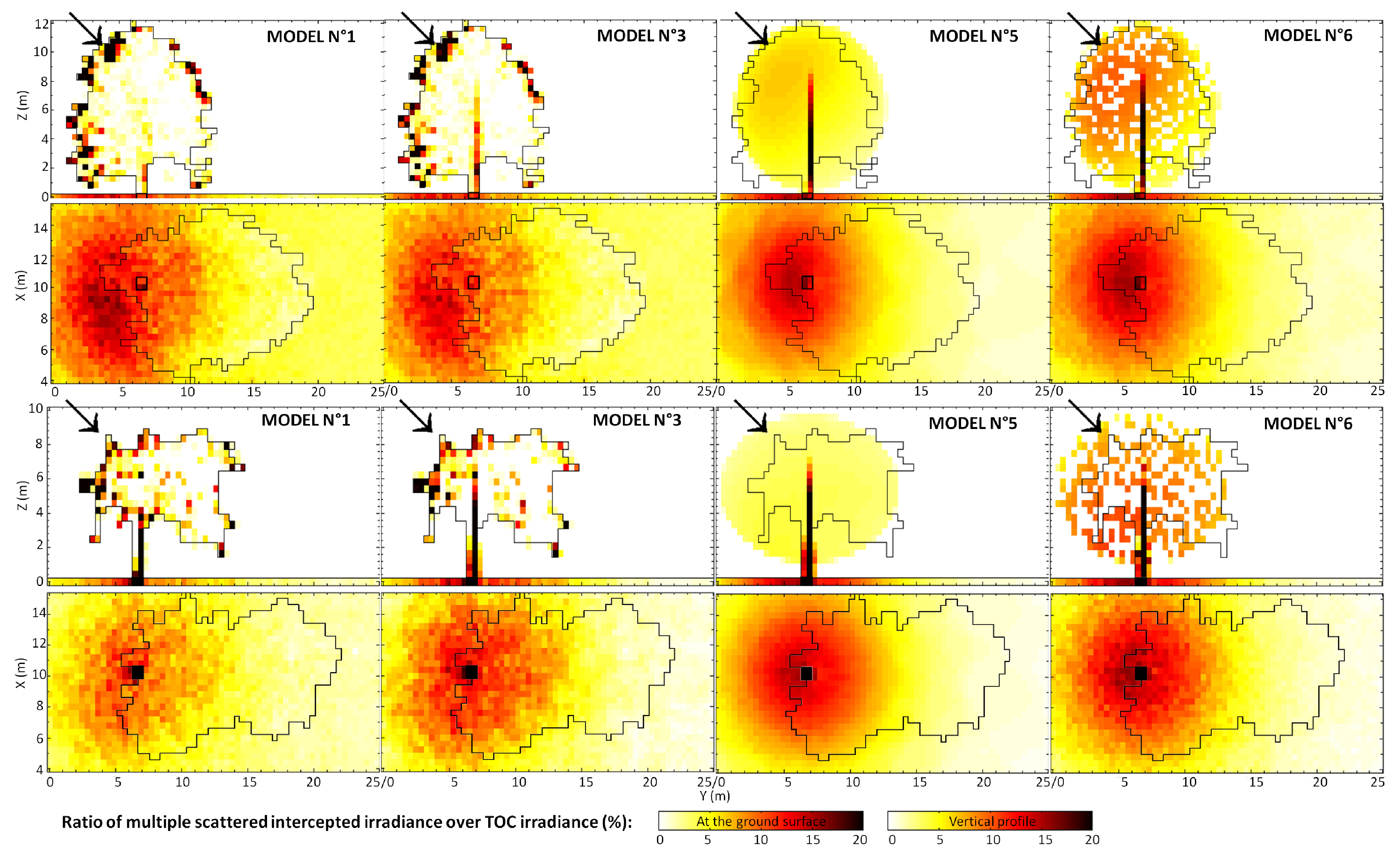
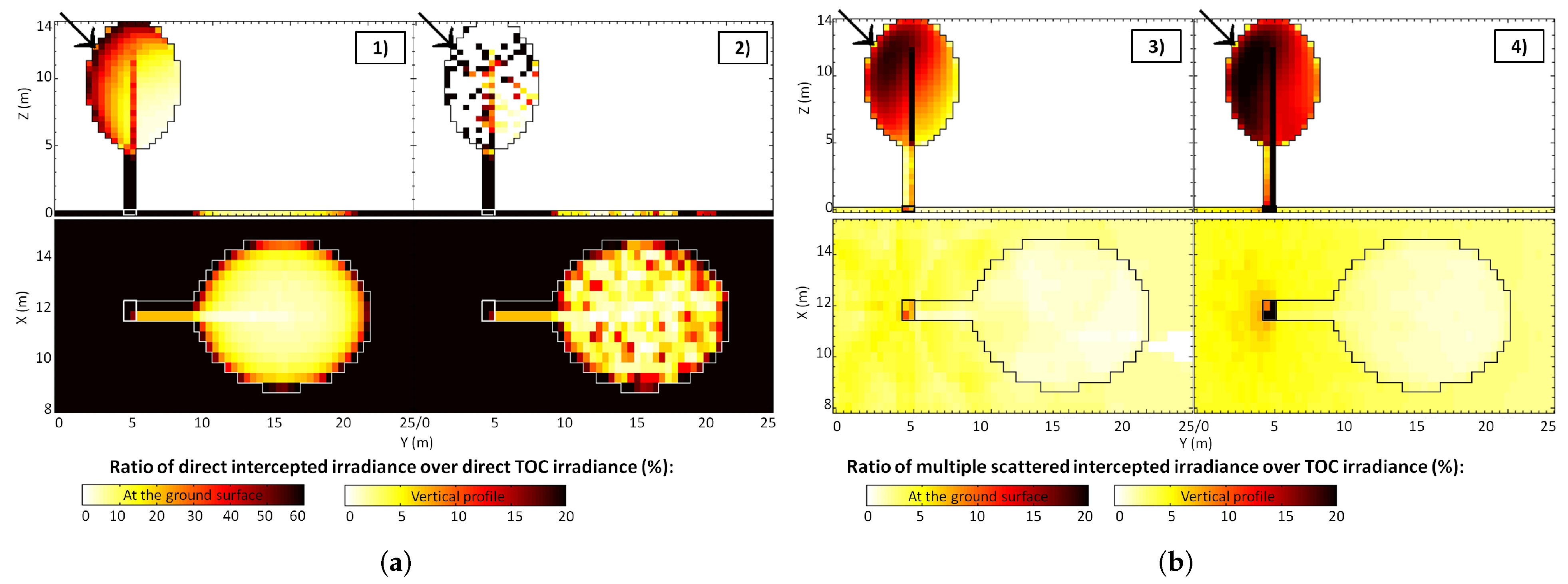
3.2.2. Spatial Analysis

On one side for the tree models from n°1 to 6 and both the magnolia and linden trees, the downwelling direct solar radiation attenuation through the tree crown is irregular and depends on the crown 3D architecture for TLS-based and discrete voxel-grid models, whereas it is more gradual for the geometric ones, except in the crown sunlit region and at NPV location due to absorption (Figure 9). Therefore, $T_{dir}$ computed in the tree shadow visually appears very heterogeneous for the first tree models and rather homogeneous for the second ones due to how LAI is distributed uniformly or not within the crown. However, the tree model n°6 having a POROSITY value larger than 0% allows slightly increasing the heterogeneous behavior of $T_{dir}$ in the shade. Then, for the linden tree, $T_{dir}$ spatial variability seems to depend only on the global crown modeling, with IQR equal to 21% for tree models n°1–3 and around 12% for tree models n°4–6 (Figure 10). For the magnolia tree, it depends on both the global crown modeling and NPV, with IQR between 25% and 27% for tree models n°1–3 and between 10% and 13% for tree models n°4–6. The multiple scattered radiation is intercepted at the crown borders where leaves are most concentrated for TLS-based and discrete voxel-grid models while it is homogeneous for the geometric n°4 and 5 models, except in the crown sunlit region and at NPV location (Figure 11). However, for the tree model n°6, the radiation penetrates deeper in the tree crown and its interception is more spread to the lowest part of the sunlit crown region. Then, the computed $T_{scat}$ is distributed at ground as a disk more or less centered on the trunk position (whose shape conforms to the projection of the tree crown) with the highest contributions located in the solar backscattering direction, depending on the presence of NPV and the height of first leaves within the crown. $T_{scat}$ ranges between 0% and 20%, with a less normal distribution than $T_{dir}$(Figure 10). For the linden tree, IQR looks similar whatever the tree model and is between 7% and 8%. For the magnolia tree, $T_{scat}$ is slightly overestimated from TLS-based compared to the other tree models. However, globally, IQR is between 4% and 6%.

On another side for the empirical tree model, the same conclusions as previously apply for the behavior of the direct solar radiation vertical interception (Figure 12a). At first order, the tree crown POROSITY and LAI play both the major role in facilitating the penetration of the radiation deeper into the crown center. In the tree shadow, POROSITY makes $T_{dir}$ spatial variations to move off a normal distribution that is skewed towards positive values (POROSITY = 30/70% gives IQR = 10/13.6%; Figure 13a). Then, high LAIs homogenize the shadow reducing $T_{dir}$ variations and, oppositely, low LAIs give a more heterogeneous shadow (LAI = 1/6 m².m⁻² gives IQR = 9.5/3.3%). Otherwise, SZA behaves in the same way as LAI in terms of influence, homogenizing the shadow the more SZA increases (SZA = 30/60° gives IQR = 7.0/2.6%). The rest of the parameters have a less significant impact. In addition, the same conclusions as previously apply for the behavior of the vertical interception of the multiple scattered radiation. An increase in BACKGROUND reflectance increases multiple scattering and leads radiation interception in the top crown sunlit region to be spread downward (Figure 12b). An increase in the shaded region is also observed for BACKGROUND being from asphalt to grass. Globally, $T_{scat}$ in the tree shadow is very low and accounts for less than 7% while $T_{dir}$ can reach until 50% in our simulations at 0.8 µm (Figure 13). The spread location of both $T_{dir}$ and $T_{scat}$ computed at ground are the same as previously mentioned. Given the low contribution of $T_{scat}$ with IQR between 0% and 3%, the influence of the parameters is not worth further analyzing for $T_{scat}$ and in this particular case of the empirical tree model.

3.3. Reflectance Retrieval Performance

First, the assessment of the reflectance retrieval performance is conducted on a mean spectral basis over 0.4–2.5 µm. The thresholds S_NB fixing the 0.02/0.03/0.04 absolute reflectance errors are retrieved at 30/45/60% for asphalt and 13/19.5/26% for grass. They are derived from the mean ratios $I_{trans}/I_{tot}$ computed for the TLS-based tree models. The latter globally show similar trends for the linden and the magnolia tree by accounting for the average between 80% and 85%. Then, when comparing the reference TLS-based tree models to its derived tree simplified models from n°2 to 6, NB values range between 0% and 22%. This leads in most cases to good reflectance retrieval performances for both discrete and geometric voxel-grid tree models (

Table 5. Comparison of the normalized mean bias NB expressed in % between the two reference tree models and different geometric tree representations (first column: T stands for the number of the compared tree models) for 6 $T_c$ observations (SZA = 30/45/60° and BACKGROUND = A – asphalt / G – grass) and the two tree species. NB values are highlighted in green/yellow/orange/red for respectively good/acceptable/critical/unacceptable reflectance retrieval performances when compared to the according thresholds $S_{NB}$.

	Reference: TLS-Based Tree Model n°1
	Linden						Magnolia
T	30°/A	30°/G	45°/A	45°/G	60°/A	60°/G	30°/A	30°/G	45°/A	45°/G	60°/A	60°/G
2	0	0	0.2	0.2	0	0	12	11.7	15.4	15.1	20.2	20
3	2.8	3	3.6	3.8	5.1	5.2	10.5	10.3	13.8	13.5	15.8	15.6
4	21.8	21.2	14	14	13	13.2	6.2	5.9	4	4	4.3	4.3
5	20.8	20.2	13.4	13.4	10.4	10.6	1.3	1.4	4.6	4.6	4.5	4.4
6	18.6	18.1	11.1	11.1	10.4	10.6	4.4	4.4	7.6	7.4	7.4	7.3
	Reference: Empirical Tree Model E
	Linden						Magnolia
T	30°/A	30°/G	45°/A	45°/G	60°/A	60°/G	30°/A	30°/G	45°/A	45°/G	60°/A	60°/G
1	51.3	52.8	39	40.5	74.1	74.5	18.9	20.2	3.4	4.7	35.1	35.7
4	38.5	40.8	29.5	31.4	71.1	71.5	20	21.3	7.7	8.8	37.9	38.4

). Nevertheless, acceptable to critical performances are sometimes observed for the geometric ones and the linden tree when BACKGROUND = grass, and for the discrete ones for the magnolia tree when BACKGROUND = grass and SZA > 30°. When comparing predicted $T_c$ from the reference empirical tree model with simulated $T_c$ from tree models n°1 and 4, a large majority of NB values are higher than 20%. Except for few cases which show good reflectance retrieval performances essentially for the magnolia tree, performances from acceptable to unacceptable are most often observed, above all with BACKGROUND = grass and whatever the SZA values.

Secondly, the impact of neglecting $T_{dir}$ or $T_{scat}$ on reflectance retrieval accuracy is studied for the reference TLS-based tree models and two specific spectral bands with grass as the background type. Consequently, a new computation of the thresholds $S_{NB}$ is needed. It is further based on an analysis of the irradiance radiation budget in the tree shadow for the two tree species. The latter shows that the spectral contribution of $I_{trans}^{dir,d}$ and $I_{coup}$ is negligible: the first accounting for 0.5–4.5% and the second for less than 1% of $I_{tot}$ (data not shown). On the contrary, the fraction of $I_{trans}^{dir,d}$ in $I_{tot}$ is the first contributor followed by $I_{trans}^{scat}$ and $I_{dif}$ (Figure 14). $I_{trans}^{dir,s}$ is monotonously increasing with the wavelength and reaches in the average 45–70% in the visible, 65–80% in the NIR, and 80–95% in the SWIR. $I_{trans}^{scat}$ is spectrally dependent and its spectral variations follows those of LOP over 0.4–2.5 µm (cf. Figure 1). It is close to 0% in the visible, between 10% and 20% in the NIR, and from 0% to 15% in the SWIR. Then, the ratio $I_{trans}/I_{tot}$ gives 74/73% in the red band and 83/82% in the NIR band for the linden/magnolia tree, leading to the following $S_{NB}$ values: 60/90/120% in the red and 5/7/10% in the NIR for the linden, 32/49/65% in the red and 3/5/7% in the NIR for the magnolia tree. Finally, whatever the tree species and the tree model, the results point out that neglecting $T_{scat}$ at 0.67 µm still leads to good reflectance retrieval performances (

Table 6. Comparison of the normalized mean bias NB expressed in % between the reference TLS-based tree models and all tree models (first column: T stands for the number of the compared tree models) by either neglecting $T_{dir}$ or $T_{scat}$ at two spectral bands for the two tree species (SZA = 45° and BACKGROUND = grass). NB values are highlighted in green/yellow/orange/red for respectively good/acceptable/critical/unacceptable reflectance retrieval performances when compared to the according thresholds $S_{NB}$.

	Neglecting Tdir				Neglecting Tscat
	Linden		Magnolia		Linden		Magnolia
T	Red (0.67 µm)	NIR (0.8 µm)	Red (0.67 µm)	NIR (0.8 µm)	Red (0.67 µm)	NIR (0.8 µm)	Red (0.67 µm)	NIR (0.8 µm)
1	99.6	75.6	99.5	89.5	16.4	10.5	7.6	4.0
2	99.6	75.6	99.1	85.5	16.4	10.6	9.6	6.4
3	99.6	77.0	99.4	88.4	14.5	10.6	12.0	21.4
4	99.5	75.8	99.2	87.3	9.9	30.0	5.3	20.9
5	99.6	75.8	99.2	87.2	10.8	30.8	6.3	21.7
6	99.6	76.3	99.1	86.9	10.3	30.0	3.0	19.4

). However, unacceptable ones are obtained at 0.8 µm, with punctual exceptions for the tree models n°1 and 2. Neglecting $T_{dir}$ leads to the worst NB values and so unacceptable performances for the two tree species, all the tree models, and the two studied spectral bands. One exception applies for the linden at 0.67 µm, giving critical performances.

4. Discussion

4.1. Impact of the 3D Tree Modeling from Realistic Scenarios on the Simulated Tree Crown Transmittance

The optimal choice of the tree 3D representation depends on the available means of acquisition or observation. On one side, TLS and ALS acquisitions enable to get the exact description of the distribution of the crown materials (i.e., leaves and NPV), necessary to build the tree model n°1, and then the tree models n°2 and 3 [30]. However, these measurements are laborious, expensive, and not always available. On another side, a rough tree modeling as with the tree models n°4 and 5 is more easy to obtain and more flexible, from allometric equations or coarse determination of crown dimensions and tree height derived from IS and 3D data [17]. At the opposite, the tree model n°6 is less accommodating because the knowledge of the tree crown porosity, here used as a proxy for leaf clumping, is hard to measure or derive from ancillary data. However, it should be or assumed to be a better representation than the tree models n°4 and 5.

The spectral and spatial analysis of simulated $T_c$ computed in the tree shadow for the abstract tree models showed the following conclusions when compared to the reference TLS-based tree models n°1. Whatever the tree model, the spectral shape of $T_c$ is preserved, attesting that $T_{scat}$ is well simulated in the average. However, a constant positive or negative shift in T_c spectral magnitude is observed, which is due to errors in $T_{dir}$ simulations. Then, discrete voxel-grid tree models conform much better to $T_c$ spatial distribution in the tree shadow than geometric ones. Because geometric models tend to homogenize the tree shadow and so smooth sunflecks, the dispersion of $T_{dir}$ distribution decreases by a factor of around 2 compared to the discrete models. On the contrary, $T_{scat}$ distributions are quite similar, showing that they are rather independent of the tree model. This is explained because they represent a small contribution within the shadow borders (unlike $T_{dir}$) since they are more dispersed within the projection of the tree crown at ground, where multiple scattering is enhanced on the radiation path length by a larger volume of leaves and NPV. The trunk being a higher reflective material compared to leaves on the average, the highest magnitude of $T_{scat}$ is found in front of the trunk in the solar backscattering direction. Furthermore, whatever the discrete or geometric tree model, the decrease in NPV fraction modeling (from TLS-based trunk and branches to cylindrical trunk) generally overestimates $T_c$ the more the tree LAI decreases. These results for the magnolia tree are in agreement with [30,55] because the crown transmits more radiation with less NPV and present less multiple scattering, which leads to higher $T_{dir}$ and lower $T_{scat}$ (and, thus, a global $T_c$ overestimation because $T_{dir}$>>$T_{scat}$). For the linden tree, the NPV reconstruction from the TLS measurements was not fully complete due to the high leaf volume obstructing the laser beam penetration. Therefore, the fraction of NPV is slightly increased from the TLS-based triangle representation to the cylinder one, which produces an unrealistic $T_c$ underestimation that actually remains low. At last, in function of the observation conditions, the impact of the background type on simulated $T_c$ is negligible for the tree models. This proves that the fraction of multiple scattered irradiance between the background and the crown is low compared to this coming from crown multiple scattering. In turn, the impact of SZA is more significant. For the magnolia tree and high SZA, leaf clumping and penumbra effects increase since the shadow becomes larger at ground. For the linden tree and low SZA, the shadow is mostly located under the crown and so $T_c$ bias increases with a more abstract tree crown modeling.

In summary, for a low LAI (here magnolia, LAI = 1.28 m².m⁻² and crown porosity = 60%), the accuracy of simulating $T_c$ the closest to the one from the TLS-based tree models is sensitive to the tree global geometry shape and the NPV modeling (differences between the tree models n°2–3 and n°4–5). For a slight increase in LAI and a sharp decrease in crown porosity (here linden, LAI = 2.27 m².m⁻² and crown porosity = 28.5%), only the tree global geometry shape is the major factor of sensitivity. In addition, the results reveal that the tree model n°6 was not systematically better than the tree models n°4 and 5, as expected. Possibly, this clumping correction type is not adapted for the geometric models. Leaf clumping is better modeled with the discrete tree models, but with a strong influence of the digitization step of the tree crown (i.e., the voxel size) [30,61]. Globally for the magnolia, the geometric tree models seem more appropriate than the discrete ones. However, [30] showed that discrete models are the most suited whatever the tree LAI when working at high spatial resolution (<1 m) in the case of a savanna broadleaf open forest. The authors of [39] also showed that a discrete model performs better than a geometric one for a dense coniferous/broadleaf forest (mean PAI of 5.5 m².m⁻²; voxel size = 2 m). For the magnolia case, differences might come from the voxel size fixed to 0.4 m in our study that might be too coarse. For the linden, the discrete tree models are very close to the reference TLS-based tree model and so appear to be the most suitable. Actually, the geometric tree models may be a too simple representation given a porosity that is not negligible and whose impact on $T_c$ increases with the tree LAI.

4.2. Limitations of the Empirical Tree Model to Predict the Tree Crown Transmittance

Due to the high diversity of species and morphologies (as seen for the magnolia and linden in this study), it is not concretely possible to define a 3D tree model able to take into account all spectral and structural tree properties for the sake of generalization. Therefore, an empirical tree model was defined with a fixed geometry to be as simple as possible, but highly unlikely to be realistic. Nevertheless, this very simplified model can give first insights about the ability to predict $T_c$ from a statistical regression as well as its spectral and spatial behavior (work continued after [17]). For this, a sensitivity analysis showed that the global rank of influent input parameters is first the tree LAI and SZA, followed by POROSITY, ALA and its interaction with SZA. At the end for the regression, only LAI and SZA are kept as inputs. They are in agreement with the Beer–Lambert’s law and the simple theory of radiation interception [41,42]. This may be restrictive, but the difficulty is how to estimate in practical the other influent parameters from IS data? Moreover, some other non-studied parameters having a relevant impact on radiation transmission were not taken into account, such as the crown dimensions, the tree height, the presence of branches, and a heterogeneous crown leaf vertical distribution, for instance [25,55,62]. Then, from the defined empirical tree model, simulated $T_c$ was revealed to be largely dominated by $T_{dir}$, which decreases from low to high LAIs. $T_{scat}$ spectral contribution is progressively added to $T_{dir}$ only towards medium–high LAIs (≥3 m².m⁻²). A global saturation of $T_c$ appears to be achieved from LAI superior to 4 m².m⁻². A similar trend was observed by [31] for a broadleaf and conifer stand. Next, although a high nonlinear irradiance behavior is expected in tree shadow, the $T_c$ prediction performances are rather good (RMSE ≤ 4.3%, R² ≥ 0.91, absolute maximum bias ≤ 10%). In comparison to [17], the prediction of the ratio $I_{trans}/I_{tot}$ with a similar expression as Equation 5 gave similar performances (RMSE ≤ 8.3%, R² ≥ 0.87), but with higher absolute maximum bias up to 20%. This might be due to the higher variability of $I_{tot}$ than $I_{TOC}\left(T_c=I_{trans}/I_{TOC}\right),$ which demonstrates that using $T_c$ may lead to lower reflectance bias than $I_{trans}/I_{tot}$ for atmospheric correction purposes.

The spectral and spatial analysis of simulated and predicted $T_c$ in tree shadow for the empirical tree model compared to the reference TLS-based tree models n°1 showed the following conclusions. The mean spectral $T_c$ is always underestimated with predicted $T_c$ because of a systematic underestimation of both $T_{scat}$ and $T_{dir}$ that increases with the LAI. On one side for $T_{dir}$ and its spatial distribution in the tree shadow, POROSITY also plays an important role in addition to LAI and SZA. However, it was not selected as an input for the empirical regression. Thus, a possible explanation of the wrong predictions of $T_c$ may come from the fact to have neglected the impact of POROSITY combined with an erroneous tree global geometry shape. For instance, the tree height as well as the crown volume (dimensioned by crown height and (x,y) diameters) modify the path length of $I_{trans}$ through the tree crown, and so the calculation of $T_c$ [42]. Actually, differences in tree height and crown volume between the empirical tree model and the reference TLS-based ones account for 4.72/2.64 m and 162/492 m³ for the magnolia/linden tree respectively. In comparison, the other tree abstract models have maximum changes in tree height of 0.17/0.34 m and crown volume of 365/143 m³ against the references. Therefore, for $T_{dir}$, there is an increasing order of spatial distribution deviations from TLS-based tree models to discrete ones, then geometric ones and, at last, the empirical one. In parallel, the interquartile range of $T_{dir}$ at 0.8 µm is similar between the TLS-based and discrete models (IQR of 21/25–27% for the linden/magnolia tree), starts to differ from the TLS-based for the geometric ones (IQR of 12/10–13%) and increasingly differ for the empirical tree model (IQR ≤ 8% for tree LAI ≥ 1 m².m⁻²). On another side, the comparison of $T_{scat}$ spatial distribution at shadow is rather similar whatever the tree model. However, the interquartile range at 0.8 µm showed an IQR of 7–8%/4–6% for linden/magnolia and for TLS-based, discrete, and geometric tree models, and an IQR of 0–3% for the empirical one. Actually being dispersed under the tree crown, $T_{scat}$ distribution depends on the crown projected area. However, this latter differs from 89/91 m² for the empirical tree model compared to the TLS-based tree models for the magnolia/linden, while for the other tree models, it only differs at maximum from 19/22 m². As such, $T_{scat}$ is also influenced by the tree global geometry shape for the same reasons as $T_{dir}$. Apart from this, $T_{scat}$ magnitude is very low for the empirical tree model, and so the impact of the input parameters remains globally very low. Nonetheless, this could have changed if this impact was studied for the tree 3D modeling from the realistic scenarios.

At the end, comparing the empirical tree model with more realistic tree representations showed that the most important sources of error in estimating $T_c$ are ranked in decreasing order: (1) the accuracy in the global tree geometry shape, accounting for crown dimensions, clumping and tree height (mean spectral bias of 3.7–21.5% between the empirical and the geometric tree model n°4), (2) the accuracy in estimating $T_{scat}$ (errors until 13% in the average at 0.8 µm where $T_{scat}$ is close to maximum), and (3) the degree of realism for the 3D tree representation (mean spectral bias until 7.5% between the TLS-based and the geometric tree model n°4). One should note that these errors are not independent one from another and are only valid for the two studied trees.

4.3. Impact of the Tree Crown Transmittance on Surface Reflectance Retrieval in the Tree Shadow

On a mean spectral basis over 0.4–2.5 µm, all abstract tree models derived from the TLS-based ones demonstrated good reflectance retrieval performances (error < 0.02), except when the highest normalized biases are combined with grass as background (acceptable to critical performances with error between 0.02 and 0.04). Otherwise, the use of the statistical regression to predict $T_c$ from the empirical tree model leads to good to unacceptable performances compared to the TLS-based and the geometric tree model n°4. The presence of grass regardless of SZA values gives the lowest performance. In comparison with literature for a single tree casting a shadow on grass, errors of 0.010/0.018/0.280 in retrieved reflectance at respectively 0.45/0.65/0.75 µm using ATCOR-4 atmospheric correction code (SZA = 30.2°, IS data at 2 m)were shown [4]. With the same dataset over 0.4–0.9 µm and for a different tree species, the authors of [5] observed an average normalized bias of 37.5% compared to sunlit regions by using an atmospheric correction approach, accounting only for diffuse irradiance in the shade. This error can reach up to 56.5% at 0.7 µm. Another approach was tested by using DART and a discrete voxel-grid tree model (voxel size = 2 m, no NPV) by computing scaling factors for fractions of direct/diffuse irradiance in the shade. An improved average normalized bias of 9.6% is found with a highest deviation of 35.5% close to 0.7 µm. Based on our reflectance retrieval performance ranking, the authors of [4] presented good performances in the visible and unacceptable ones in the NIR. In [5], they are unacceptable for the first approach and good to unacceptable depending on the spectral band for the second one. The results of these studies are in agreement with our results. In a different situation when ground reflectance is higher such as for snow, the issue of the impact of canopy shading on albedo variation is also raised by [63] and probably enhanced compared to grass. When ground reflectance is lower such as for asphalt, errors in retrieved reflectance decrease by a factor of 30% compared to grass, while for water having a mean reflectance lower than 0.04, atmospheric correction is much more challenging (SZA = 55–57°, IS data at 0.8 m) [17]. At last, apart from the background impact, the authors of [30] also pointed out that high SZA values generate important biases in TOC reflectance retrieval and, thus, in ground reflectance.

Now, by accounting the spectral contribution of $T_{dir}$ or $T_{scat}$ into $T_c$, both are spectrally dependent over 0.4–2.5 µm (studied case: SZA = 45°, grass). $T_{dir}$ increases from lower to higher wavelengths by 40%, whereas the T_scat spectral shape fits the one of LOP and can globally reach until 20% in our study. Neglecting $T_{dir}$ at the red band (0.67 µm) leads to critical to unacceptable reflectance retrieval performances in the tree shadow. This is because $T_{dir}$ ≈ $T_c$≈ 73/74% for the magnolia/linden. Thus, neglecting $T_{scat}$ is largely acceptable in the red band. The authors of [4] found, on the contrary, good performances. However, the difference might be due to a higher tree LAI (with the empirical tree model, a tree LAI of 6 m².m⁻² gives a mean $T_{dir}$ of 1%). Neglecting either $T_{dir}$ or $T_{scat}$ at the NIR band (0.8 µm) presents unacceptable performances, in agreement with [4,5]. Then, neglecting only $T_{scat}$ with the TLS-based and the discrete tree models with the triangle NPV representation showed from acceptable to critical performances. With further comparison with literature, the authors of [30] showed that the fraction of TOC reflectance coming from $T_{dir}$ contribution was underestimated in the tree shadow between a TLS-based and a discrete tree model (voxel size = 0.3 m, SZA = 45°, 1 m simulated spatial resolution, dry bare soil). This underestimation was very slightly increased from red to NIR band and clearly increased with the tree LAI from 0.75, 2.02, to 7.16 m².m⁻². This result is in line with our study showing a slight $T_{dir}$ increase of 1/9% for linden/magnolia between red and NIR (based on Figure 14), the increase following the tree LAI being not possible to be judged because of the large dependency of different clumping per individual tree. For a linden tree and a discrete tree model (voxel size = 0.25 m, SZA = 25–30°, grass), the authors of [6] found that a decrease of irradiance in the green band due to the presence of the tree was noticeable both in the tree shadow and the crown shaded side, while in the NIR, this decrease was only observed in the tree shadow, whereas an increase was discerned within the tree crown outlines essentially in the sunlit side and in front of the tree oppositely to the tree shadow. These results can be explained in our study by the main influence of $T_{dir}$ in the green and both $T_{dir}$ and $T_{scat}$ in the NIR. Actually, $T_{scat}$ increases the total irradiance due to crown multiple scattering, mainly on the crown sunlit side and within the ground projection of the tree crown, essentially in the solar backscattering direction. In addition, $T_{scat}$ tends to increase with the tree LAI (for [6], the tree LAI was 8.4 m².m⁻²). Finally, the comparison of these results with those of this paper is not straightforward because often the tree LAI is unknown, the spatial resolution, the background type and SZA are different, the voxel size is not the same (from 0.25 to 2 m) as well as the tree modeling type.

Next, considering that the goal further tackled by this study is to improve the reflectance correction in the tree shadow by the 3D atmospheric correction models, especially the ICARE-VEG model from [17], the following challenges have been raised by using an empirical tree modeling: (i) take into account in the statistical regression predicting $T_c$ the tree global geometry shape, the leaf clumping (for low/high LAI), and the NPV fraction (for low LAI) in addition to LAI and SZA, in order to better approach the performance of the geometric voxel-grid tree model n°4 (hopefully a better prediction of $T_{scat}$ is expected at least and also of $T_{dir}$); (ii) try to investigate a method not decoupling the spectral and spatial variations of $T_c$ to build the physics-based atmospheric correction factor; (iii) extend the spectral and spatial analysis with new realistic trees of varying tree LAIs (notably higher than this of the linden); and (iv) develop a strategy to switch from geometric tree models derived from IS and 3D data to discrete tree models with a particular attention to be paid on the appropriate choice of the voxel size.

5. Conclusions

Accurate ground reflectance retrieval in tree shadows from IS data at high spatial resolution is still an ongoing and challenging issue, particularly for 3D atmospheric correction codes. In this paper, its performance is assessed through the study of the tree crown transmittance $T_c$, when predicted or simulated from different levels of abstraction of tree models built from TLS measurements. The spectral and spatial variability of $T_c$ is further decomposed into its direct non-intercepted contribution, $T_{dir}$, and its multiple scattering contribution, $T_{scat}$. The results derived from this preliminary and non-exhaustive study aim at giving the orders of magnitude of the sources of error to estimate $T_c$ correctly, and new ways of improvements for atmospheric correction codes to deal with reflectance retrieval in tree shadows. For the first point, we conclude that although a statistical regression coming from a simplified empirical tree model showed good performance in predicting $T_c$ (RMSE ≤ 4.3%, R² ≥ 0.91), it globally fails when compared to tree models from more realistic scenarios because in order of importance: (1) the global tree geometry shape has not been taken into account (mean spectral bias of 3.7–21.5%), (2) $T_{scat}$ is always underestimated (errors until 13% in the average), and (3) the degree of realism for the 3D tree representation is not properly respected (mean spectral bias until 7.5%). Therefore, in order to bring improvements, the statistical regression should include, as main factors, the global tree geometry (crown/tree dimensions), the leaf clumping and the wood fraction in addition to the tree LAI and the solar zenith angle. The IS data from [17,64,65,66] gave perspectives to estimate some of these, such as stem volume per crown area, DBH and crown area, LAI and clumping index, tree height and crown diameter, respectively. Moreover, although a geometric voxel-grid tree modeling is easy to implement (as done with the empirical tree model), it showed its limitations compared to TLS-based tree models, unlike discrete voxel-grid ones. The major sources of error come from the leaf clumping modeling in relation to the voxel size, and the wood 3D representation. Then, in any case, whatever the tree modeling type, increasing values of tree LAI and solar zenith angle greatly impact the magnitude of these sources of error. Furthermore, $T_{scat}$ contribution needs to be considered in addition to $T_{dir}$ for accurate reflectance retrieval, essentially for the spectral bands sensitive to the variations of the leaf optical properties over 0.4–2.5 µm. Generally, neglecting $T_c$ or only $T_{scat}$ in NIR and SWIR leads to unacceptable reflectance retrieval results, in particular, the more the background reflectance increases. In summary for atmospheric correction purposes, this study stresses both the need to use discrete voxel-grid tree modeling instead of geometric voxel-grid ones, and the need to know how to approximate the spectral and spatial variability of both $T_{dir}$ and $T_{scat}$ contributions. At last, these previous conclusions are worthwhile for the two studied trees: a magnolia and a linden tree. However, they need to be extended to other trees with different tree LAIs (attention should be paid to $T_c$ saturation achieved at LAI > 4 m².m⁻²) and validated with additional in situ field measurements (such as irradiance field data as performed by [6], or building appropriate protocols to directly measure $T_c$ spectrally over 0.4–2.5 µm). In addition, the variations of the leaf optical properties according to their crown vertical distribution have not been analyzed in this study, but their influence on $T_c$ may play a role and deserve to be examined in the future. Finally, all these previous further investigations will help in deriving the most appropriate atmospheric correction factor in tree shadow (possibly at an operational level) to have a better determination of reflectance and, thus, a better derivation of physical variables from IS data for land cover mapping in urban areas, and both vegetation and soil monitoring in natural ecosystems.

References

1. Ustin, S.L.; Roberts, D.A.; Gamon, J.A.; Asner, G.P.; Green, R.O. Using imaging spectroscopy to study ecosystem processes and properties. Bioscience 2004, 54, 523–534. [Google Scholar] [CrossRef]
2. Chabrillat, S.; Ben-Dor, E.; Cierniewski, J.; Gomez, C.; Schmid, T.; Van Wesemael, B. Imaging Spectroscopy for Soil Mapping and Monitoring. Surv. Geophys. 2019, 40, 361–399. [Google Scholar] [CrossRef] [Green Version]
3. Van Der Linden, S.; Okujeni, A.; Canters, F.; Degerickx, J.; Heiden, U.; Hostert, P.; Priem, F.; Somers, B.; Thiel, F. Imaging Spectroscopy of Urban Environments. Surv. Geophys. 2019, 40, 471–488. [Google Scholar] [CrossRef] [Green Version]
4. Damm, A.; Guanter, L.; Verhoef, W.; Schlapfer, D.; Garbari, S.; Schaepman, M.E. Impact of varying irradiance on vegetation indices and chlorophyll fluorescence derived from spectroscopy data. Remote Sens. Environ. 2015, 156, 202–215. [Google Scholar] [CrossRef]
5. Fawcett, D.; Verhoef, W.; Schläpfer, D.; Schneider, F.; Schaepman, M.; Damm, A. Advancing retrievals of surface reflectance and vegetation indices over forest ecosystems by combining imaging spectroscopy, digital object models, and 3D canopy modelling. Remote Sens. Environ. 2018, 204, 583–595. [Google Scholar] [CrossRef]
6. Kukenbrink, D.; Hueni, A.; Schneider, F.D.; Damm, A.; Gastellu-Etchegorry, J.-P.; Schaepman, M.E.; Morsdorf, F. Mapping the Irradiance Field of a Single Tree: Quantifying Vegetation-Induced Adjacency Effects. IEEE Trans. Geosci. Remote Sens. 2019, 57, 4994–5011. [Google Scholar] [CrossRef]
7. Adeline, K.; Chen, M.; Briottet, X.; Pang, S.; Paparoditis, N. Shadow detection in very high spatial resolution aerial images: A comparative study. ISPRS J. Photogramm. Remote Sens. 2013, 80, 21–38. [Google Scholar] [CrossRef]
8. Gamba, P.; Lisini, G. Urban land cover mapping using hyperspectral and multispectral VHR sensors: Spatial versus spectral resolution. Proc. URBAN IAPRS 2005, 36, 1416. [Google Scholar]
9. Yuan, F.; Bauer, M.E. Mapping impervious surface area using high resolution imagery: A comparison of object-based and per pixel classification. In Proceedings of the American Society for Photogrammetry and Remote Sensing—Annual Conference of the American Society for Photogrammetry and Remote Sensing 2006: Prospecting for Geospatial Information Integration, Reno, NV, USA, 1–5 May 2006; pp. 1–5. [Google Scholar]
10. Dare, P.M. Shadow Analysis in High-Resolution Satellite Imagery of Urban Areas. Photogramm. Eng. Remote Sens. 2005, 71, 169–177. [Google Scholar] [CrossRef] [Green Version]
11. Shahtahmassebi, A.; Yang, N.; Wang, K.; Moore, N.; Shen, Z. Review of shadow detection and de-shadowing methods in remote sensing. Chin. Geogr. Sci. 2013, 23, 403–420. [Google Scholar] [CrossRef] [Green Version]
12. Richter, R.; Schläpfer, D. Geo-atmospheric processing of airborne imaging spectrometry data. Part 2: Atmospheric/topographic correction. Int. J. Remote Sens. 2002, 23, 2631–2649. [Google Scholar] [CrossRef]
13. Schläpfer, D.; Richter, R.; Feingersh, T. Operational BRDF Effects Correction for Wide-Field-of-View Optical Scanners (BREFCOR). IEEE Trans. Geosci. Remote Sens. 2014, 53, 1855–1864. [Google Scholar] [CrossRef] [Green Version]
14. Richter, R.; Schläpfer, D. ATCOR-4 User Guide; German Aerospace Center: Cologne, Germany, 2016. [Google Scholar]
15. Lachérade, S.; Miesch, C.; Boldo, D.; Briottet, X.; Valorge, C.; Le Men, H. ICARE: A physically-based model to correct at-mospheric and geometric effects from high spatial and spectral remote sensing images over 3D urban areas. Meteorol. Atmos. Phys. 2008, 102, 209–222. [Google Scholar] [CrossRef]
16. Ceamanos, X.; Briottet, X.; Roussel, G.; Gilardy, H. ICARE-HS: Atmospheric correction of airborne hyperspectral urban images using 3D information. In SPIE Remove Sensing, Proceedings of the Remote Sensing Technologies and Applications in Urban Environments II, Edinburgh, UK, 26–29 September 2006; Erbertseder, T., Esch, T., Chrysoulakis, N., Eds.; International Society for Optics and Photonics: Bellingham, WA, USA, 2016; Volume 10008, p. 100080R. [Google Scholar]
17. Adeline, K.; Briottet, X.; Ceamanos, X.; Dartigalongue, T.; Gastellu-Etchegorry, J.-P. ICARE-VEG: A 3D physics-based atmospheric correction method for tree shadows in urban areas. ISPRS J. Photogramm. Remote Sens. 2018, 142, 311–327. [Google Scholar] [CrossRef] [Green Version]
18. Sercu, B.K.; Baeten, L.; Van Coillie, F.; Martel, A.; Lens, L.; Verheyen, K.; Bonte, D. How tree species identity and diversity affect light transmittance to the understory in mature temperate forests. Ecol. Evol. 2017, 7, 10861–10870. [Google Scholar] [CrossRef]
19. Rautiainen, M.; Stenberg, P.; Nilson, T.; Kuusk, A. The effect of crown shape on the reflectance of coniferous stands. Remote Sens. Environ. 2004, 89, 41–52. [Google Scholar] [CrossRef]
20. De Castro, F.; Fetcher, N. The effect of leaf clustering in the interception of light in vegetal canopies: Theoretical considerations. Ecol. Model. 1999, 116, 125–134. [Google Scholar] [CrossRef]
21. Milenković, M.; Wagner, W.; Quast, R.; Hollaus, M.; Ressl, C.; Pfeifer, N. Total canopy transmittance estimated from small-footprint, full-waveform airborne LiDAR. ISPRS J. Photogramm. Remote Sens. 2017, 128, 61–72. [Google Scholar] [CrossRef]
22. Musselman, K.N.; Margulis, S.A.; Molotch, N.P. Estimation of solar direct beam transmittance of conifer canopies from airborne LiDAR. Remote Sens. Environ. 2013, 136, 402–415. [Google Scholar] [CrossRef]
23. Olpenda, A.S.; Stereńczak, K.; Będkowski, K. Modeling Solar Radiation in the Forest Using Remote Sensing Data: A Review of Approaches and Opportunities. Remote Sens. 2018, 10, 694. [Google Scholar] [CrossRef] [Green Version]
24. Reifsnyder, W.; Furnival, G.; Horowitz, J. Spatial and temporal distribution of solar radiation beneath forest canopies. Agric. Meteorol. 1971, 9, 21–37. [Google Scholar] [CrossRef]
25. Vales, D.J.; Bunnell, F.L. Relationships between transmission of solar radiation and coniferous forest stand characteristics. Agric. For. Meteorol. 1988, 43, 201–223. [Google Scholar] [CrossRef]
26. Hardy, J.; Melloh, R.; Koenig, G.; Marks, D.; Winstral, A.; Pomeroy, J.; Link, T. Solar radiation transmission through conifer canopies. Agric. For. Meteorol. 2004, 126, 257–270. [Google Scholar] [CrossRef]
27. Martens, S.N.; Breshears, D.D.; Meyer, C.W. Spatial distributions of understory light along the grassland/forest continuum: Effects of cover, height, and spatial pattern of tree canopies. Ecol. Model. 2000, 126, 79–93. [Google Scholar] [CrossRef]
28. Yirdaw, E.; Luukkanen, O. Photosynthetically active radiation transmittance of forest plantation canopies in the Ethiopian highlands. For. Ecol. Manag. 2004, 188, 17–24. [Google Scholar] [CrossRef]
29. Westling, F.; Underwood, J.; Örn, S. Light interception modelling using unstructured LiDAR data in avocado orchards. Comput. Electron. Agric. 2018, 153, 177–187. [Google Scholar] [CrossRef] [Green Version]
30. Widlowski, J.-L.; Côté, J.-F.; Béland, M. Abstract tree crowns in 3D radiative transfer models: Impact on simulated open-canopy reflectances. Remote Sens. Environ. 2014, 142, 155–175. [Google Scholar] [CrossRef]
31. Bartelink, H. Radiation interception by forest trees: A simulation study on effects of stand density and foliage clustering on absorption and transmission. Ecol. Model. 1998, 105, 213–225. [Google Scholar] [CrossRef]
32. Kobayashi, H.; Baldocchi, D.D.; Ryu, Y.; Chen, Q.; Ma, S.; Osuna, J.L.; Ustin, S.L. Modeling energy and carbon fluxes in a heterogeneous oak woodland: A three-dimensional approach. Agric. For. Meteorol. 2012, 152, 83–100. [Google Scholar] [CrossRef] [Green Version]
33. Verhoef, W. Light scattering by leaf layers with application to canopy reflectance modeling: The SAIL model. Remote Sens. Environ. 1984, 16, 125–141. [Google Scholar] [CrossRef] [Green Version]
34. Atzberger, C. Development of an invertible forest reflectance model: The INFORM-Model. In A Decade of Trans-European Remote Sensing Cooperation, Proceedings of the 20th EARSeL Symposium, Dresden, Germany, 14–16 June 2000; CRC Press: Boca Raton, FL, USA, 2001. [Google Scholar]
35. Gastellu-Etchegorry, J.-P.; Yin, T.; Lauret, N.; Cajgfinger, T.; Gregoire, T.; Grau, E.; Feret, J.-B.; Lopes, M.; Guilleux, J.; Dedieu, G.; et al. Discrete Anisotropic Radiative Transfer (DART 5) for Modeling Airborne and Satellite Spectroradiometer and LIDAR Acquisitions of Natural and Urban Landscapes. Remote Sens. 2015, 7, 1667–1701. [Google Scholar] [CrossRef] [Green Version]
36. Widlowski, J.-L.; Pinty, B.; Lopatka, M.; Atzberger, C.; Buzica, D.; Chelle, M.; Disney, M.; Gastellu-Etchegorry, J.-P.; Gerboles, M.; Gobron, N.; et al. The fourth radiation transfer model intercomparison (RAMI-IV): Proficiency testing of canopy reflectance models with ISO-13528. J. Geophys. Res. Atmos. 2013, 118, 6869–6890. [Google Scholar] [CrossRef] [Green Version]
37. Jacquemoud, S. Comparison of Four Radiative Transfer Models to Simulate Plant Canopies Reflectance Direct and Inverse Mode. Remote Sens. Environ. 2000, 74, 471–481. [Google Scholar] [CrossRef]
38. Fisher, R.A.; Koven, C.D.; Anderegg, W.R.L.; Christoffersen, B.O.; Dietze, M.C.; Farrior, C.E.; Holm, J.A.; Hurtt, G.C.; Knox, R.G.; Lawrence, P.J.; et al. Vegetation demographics in Earth System Models: A review of progress and priorities. Glob. Chang. Biol. 2018, 24, 35–54. [Google Scholar] [CrossRef] [PubMed] [Green Version]
39. Schneider, F.D.; Leiterer, R.; Morsdorf, F.; Gastellu-Etchegorry, J.-P.; Lauret, N.; Pfeifer, N.; Schaepman, M.E. Simulating imaging spectrometer data: 3D forest modeling based on LiDAR and in situ data. Remote Sens. Environ. 2014, 152, 235–250. [Google Scholar] [CrossRef]
40. Adeline, K.R.M.; Briottet, X.; Paparoditis, N.; Gastellu-Etchegorry, J.-P. Material reflectance retrieval in urban tree shadows with physics-based empirical atmospheric correction. In Proceedings of the Joint Urban Remote Sensing Event 2013, Sao Paulo, Brasil, 21–23 April 2013; pp. 279–283. [Google Scholar]
41. Nilson, T. A theoretical analysis of the frequency of gaps in plant stands. Agric. Meteorol. 1971, 8, 25–38. [Google Scholar] [CrossRef]
42. Norman, J.M.; Welles, J.M. Radiative Transfer in an Array of Canopies. Agron. J. 1983, 75, 481–488. [Google Scholar] [CrossRef]
43. Adeline, K.R.M.; Le Bris, A.; Coubard, F.; Briottet, X.; Paparoditis, N.; Viallefont, F.; Rivière, N.; Papelard, J.-P.; David, N.; Déliot, P.; et al. Description de la campagne aéroportée UMBRA: Étude de l’impact anthropique sur les écosystèmes urbains et naturels avec des images THR multispectrales et hyperspectrales: Urban Material characterization in the sun and shade of Built-up structures and tree. Rev. Française Photogrammétrie Télédétection 2013, 202, 79–92. [Google Scholar]
44. Miller, J.R.; Steven, M.D.; Demetriades-Shah, T.H. Reflection of layered bean leaves over different soil backgrounds: Measured and simulated spectra. Int. J. Remote Sens. 1992, 13, 3273–3286. [Google Scholar] [CrossRef]
45. Rivière, N.; Anna, G.; Hespel, L.; Tanguy, B.; Velluet, M.-T.; Frédéric, Y.-M. Modeling of an active burst illumination imaging system: Comparison between experimental and modelled 3D scene. In Proceedings of the Electro-Optical Remote Sensing Photonic Technologies, and Applications IV, Toulouse, France, 8 October 2010; p. 783509. [Google Scholar] [CrossRef]
46. Béland, M.; Widlowski, J.-L.; Fournier, R.A.; Côté, J.-F.; Verstraete, M.M. Estimating leaf area distribution in savanna trees from terrestrial LiDAR measurements. Agric. For. Meteorol. 2011, 151, 1252–1266. [Google Scholar] [CrossRef]
47. Nowak, D.J. Estimating leaf area and leaf biomass of open-grown deciduous urban trees. For. Sci. 1996, 42, 504–507. [Google Scholar] [CrossRef]
48. De Wit, C.T. Photosynthesis of Leaf Canopies; Pudoc: Wageningen, The Netherlands, 1965; ISBN 0-7923-6334-5. [Google Scholar]
49. Wang, Y.; Lauret, N.; Gastellu-Etchegorry, J.-P. DART radiative transfer modelling for sloping landscapes. Remote Sens. Environ. 2020, 247, 111902. [Google Scholar] [CrossRef]
50. Wang, Y.; Gastellu-Etchegorry, J.-P. DART: Improvement of thermal infrared radiative transfer modelling for simulating top of atmosphere radiance. Remote Sens. Environ. 2020, 251, 112082. [Google Scholar] [CrossRef]
51. Wang, Y.; Gastellu-Etchegorry, J.-P. Accurate and fast simulation of remote sensing images at top of atmosphere with DART-Lux. Remote Sens. Environ. 2021, 256, 112311. [Google Scholar] [CrossRef]
52. Gastellu-Etchegorry, J.-P.; Lauret, N.; Yin, T.; Landier, L.; Kallel, A.; Malenovsky, Z.; Al Bitar, A.; Aval, J.; BenHmida, S.; Qi, J.; et al. DART: Recent Advances in Remote Sensing Data Modeling with Atmosphere, Polarization, and Chlorophyll Fluorescence. IEEE J. Sel. Top. Appl. Earth Obs. Remote Sens. 2017, 10, 2640–2649. [Google Scholar] [CrossRef]
53. McPherson, E.G.; Rowntree, R.A. Geometric solids for simulation of tree crowns. Landsc. Urban Plan. 1988, 15, 79–83. [Google Scholar] [CrossRef]
54. Larsen, M.; Eriksson, M.; Descombes, X.; Perrin, G.; Brandtberg, T.; Gougeon, F.A. Comparison of six individual tree crown detection algorithms evaluated under varying forest conditions. Int. J. Remote Sens. 2011, 32, 5827–5852. [Google Scholar] [CrossRef]
55. Malenovský, Z.; Martin, E.; Homolová, L.; Gastellu-Etchegorry, J.-P.; Zurita-Milla, R.; Schaepman, M.E.; Pokorný, R.; Clevers, J.G.; Cudlín, P. Influence of woody elements of a Norway spruce canopy on nadir reflectance simulated by the DART model at very high spatial resolution. Remote Sens. Environ. 2008, 112, 1–18. [Google Scholar] [CrossRef] [Green Version]
56. Jacquemoud, S.; Ustin, S. Modeling Leaf Optical Properties: Prospect. In Leaf Optical Properties; Amsterdam University Press: Amsterdam, The Netherlands, 2019; pp. 265–291. [Google Scholar]
57. Wallach, D.; Makowski, D.; Jones, J.W.; Brun, F. Uncertainty and Sensitivity Analysis. In Working with Dynamic Crop Models. Methods, Tools and Examples for Agriculture and Environment, 3rd ed.; Elsevier: Amsterdam, The Netherlands, 2019. [Google Scholar]
58. Olejnik, S.; Algina, J. Generalized Eta and Omega Squared Statistics: Measures of Effect Size for Some Common Research Designs. Psychol. Methods 2003, 8, 434. [Google Scholar] [CrossRef] [Green Version]
59. Burnham, K.P.; Anderson, D.R. Multimodel inference: Understanding AIC and BIC in model selection. Sociol. Methods Res. 2004, 33, 261–304. [Google Scholar] [CrossRef]
60. Gastellu-Etchegorry, J.; Grau, E.; Lauret, N. DART: A 3D Model for Remote Sensing Images and Radiative Budget of Earth Surfaces. Model. Simul. Eng. 2012, 2, 29–68. [Google Scholar] [CrossRef] [Green Version]
61. Béland, M.; Widlowski, J.-L.; Fournier, R.A. A model for deriving voxel-level tree leaf area density estimates from ground-based LiDAR. Environ. Model. Softw. 2014, 51, 184–189. [Google Scholar] [CrossRef]
62. Macfarlane, D.W.; Green, E.J.; Brunner, A.; Amateis, R.L. Modeling loblolly pine canopy dynamics for a light capture model. For. Ecol. Manag. 2003, 173, 145–168. [Google Scholar] [CrossRef]
63. Webster, C.; Jonas, T. Influence of canopy shading and snow coverage on effective albedo in a snow-dominated evergreen needleleaf forest. Remote Sens. Environ. 2018, 214, 48–58. [Google Scholar] [CrossRef]
64. Ozdemir, I. Estimating stem volume by tree crown area and tree shadow area extracted from pan-sharpened Quickbird imagery in open Crimean juniper forests. Int. J. Remote Sens. 2008, 29, 5643–5655. [Google Scholar] [CrossRef]
65. Greenberg, J.A.; Dobrowski, S.Z.; Ustin, S.L. Shadow allometry: Estimating tree structural parameters using hyperspatial image analysis. Remote Sens. Environ. 2005, 97, 15–25. [Google Scholar] [CrossRef]
66. Thomas, V.; Noland, T.; Treitz, P.; McCaughey, J.H. Leaf area and clumping indices for a boreal mixed-wood forest: Lidar, hyperspectral, and Landsat models. Int. J. Remote Sens. 2011, 32, 8271–8297. [Google Scholar] [CrossRef]
67. Weiss, M.; Baret, F.; Smith, G.; Jonckheere, I.; Coppin, P. Review of methods for in situ leaf area index (LAI) determination Part II. Estimation of LAI, errors and sampling. Agric. For. Meteorol. 2004, 121, 37–53. [Google Scholar] [CrossRef]
68. Peper, P.J.; McPherson, E.G. Evaluation of four methods for estimating leaf area of isolated trees. Urban For. Urban Green. 2003, 2, 19–29. [Google Scholar] [CrossRef]
69. Broadhead, J.; Muxworthy, A.; Ong, C.; Black, C. Comparison of methods for determining leaf area in tree rows. Agric. For. Meteorol. 2003, 115, 151–161. [Google Scholar] [CrossRef] [Green Version]
70. Miller, J.B. A formula for average foliage density. Aust. J. Bot. 1967, 15, 141–144. [Google Scholar] [CrossRef]
71. Wei, S.; Yin, T.; Dissegna, M.A.; Whittle, A.J.; Ow, G.L.F.; Yusof, M.L.M.; Lauret, N.; Gastellu-Etchegorry, J.-P. An assessment study of three indirect methods for estimating leaf area density and leaf area index of individual trees. Agric. For. Meteorol. 2020, 2020, 108101. [Google Scholar] [CrossRef]
72. Gower, S.T.; Kucharik, C.J.; Norman, J.M. Direct and Indirect Estimation of Leaf Area Index, fAPAR, and Net Primary Production of Terrestrial Ecosystems. Remote Sens. Environ. 1999, 70, 29–51. [Google Scholar] [CrossRef]
73. Moorthy, I.; Miller, J.R.; Berni, J.A.J.; Zarco-Tejada, P.J.; Hu, B.; Chen, J. Field characterization of olive (Olea europaea L.) tree crown architecture using terrestrial laser scanning data. Agric. For. Meteorol. 2011, 151, 204–214. [Google Scholar] [CrossRef]
74. Villalobos, F.; Orgaz, F.; Mateos, L. Non-destructive measurement of leaf area in olive (Olea europaea L.) trees using a gap inversion method. Agric. For. Meteorol. 1995, 73, 29–42. [Google Scholar] [CrossRef]
75. White, M.A.; Asner, G.P.; Nemani, R.R.; Privette, J.L.; Running, S.W.; Privette, J. Measuring Fractional Cover and Leaf Area Index in Arid Ecosystems: Digital camera, radiation transmittance, and laser altimetry methods. Remote Sens. Environ. 2000, 74, 45–57. [Google Scholar] [CrossRef]
Figure 1. Digital camera pictures of the two trees (top left side: magnolia; top right side: linden) and mean spectral properties of their trunk and leaves (bottom side: “leaf 1” stands for reflectances and “leaf 2” stands for 1 − transmittance).
Remotesensing 13 00931 g001
Figure 2. General methodological workflow.
Remotesensing 13 00931 g002
Figure 3. DART 3D mockups of the tree models and NPV (i.e., trunk and branches) for the two species (for global interpretation, dimensions are not respected). Leaves are either represented by triangles (light green color) in the TLS-based tree model n°1 or simulated as a 3D distribution of voxels filled with turbid medium (dark green color) in the discrete voxel-grid tree model n°2 and the geometric voxel-grid tree models n°4 and E. NPV (brown color) are either represented by triangles for the TLS-based and discrete/geometric voxel-grid tree models n°1, 2, and 4 or a cylinder followed by a cone for the discrete/geometric voxel-grid tree models n°3, 5, and 6.
Remotesensing 13 00931 g003
Figure 4. Optical properties of the DART scene background (reflectance, and both the trunk (reflectance) and leaves (reflectance and 1 − transmittance) for the empirical tree model E. Differences in the number of displayed dots are due to the fact that the spectra do not have the same number of wavelengths. DART applies an interpolation for wavelengths where the spectrum value is not provided.
Remotesensing 13 00931 g004
Figure 5. Sensitive index η2 computed for each input parameter alone or in interactions (contribution in the variability of the output, that is the tree crown transmittance) for different LAI ranges, (a) low: 0.5 m2.m−2 ≤ LAI ≤ 2 m2.m−2, (b) medium: 2 m2.m−2 ≤ LAI ≤ 3.5 m2.m−2 and (c) high: 3.5 m2.m−2 ≤ LAI ≤ 8 m2.m−2 for the empirical tree model.
Remotesensing 13 00931 g005
Figure 6. Spectral variations of the tree crown transmittance for LAI equal to (a) 1 m2.m−2, (b) 3 m2.m−2 and (c) 6 m2.m−2 for the empirical tree model.
Remotesensing 13 00931 g006
Figure 7. Spectral validation of tree crown transmittance between predictions and simulations for the empirical tree model.
Remotesensing 13 00931 g007
Figure 8. Comparison of the simulated mean tree crown transmittances for the tree models from n°1 to 6 and the predicted one from the empirical tree model, for (a) the linden and (b) the magnolia tree (SZA = 45° and BACKGROUND = grass).
Remotesensing 13 00931 g008
Figure 9. Ratio of the direct intercepted irradiance over the direct I T O C through a vertical profile at X = 10 m (first/third rows) and T d i r computed at the ground surface Z = 0 m (second/fourth rows) for the linden (two first rows) and magnolia trees (two last rows) at 0.8 µm (SZA = 45° and BACKGROUND = grass; solar direction indicated by the black arrow, crown spatial extents delineated in black, shadow and trunk location in white).
Remotesensing 13 00931 g009
Figure 10. Boxplots of T d i r and T s c a t representing their spatial variations computed within the tree shadow delineations at ground for the different tree models of the linden and magnolia trees at 0.8 µm (SZA = 45° and BACKGROUND = grass; red/blue dots: mean/standard deviation).
Remotesensing 13 00931 g010
Figure 11. Ratio of the multiple scattered intercepted irradiance over I T O C through a vertical profile at X = 10 m (first/third rows) and T s c a t computed at the ground surface Z = 0 m (second/fourth rows) for the linden (two first rows) and magnolia trees (two last rows) at 0.8 µm (SZA = 45° and BACKGROUND = grass; solar direction indicated by the black arrow, crown spatial extents delineated in black, shadow and trunk location in black).
Remotesensing 13 00931 g011
Figure 12. Ratio of the direct and multiple scattered intercepted irradiance over I T O C through a vertical profile at X = 11.2 m (first row) and (a) T d i r or (b) T s c a t computed at the ground surface Z = 0 m (second row) for the empirical tree model at 0.8 µm with (1) and (3) the base simulation scenario, (2) POROSITY = 70% and (4) BACKGROUND = grass (solar direction indicated by the black arrow, crown spatial extents delineated in black, shadow and trunk location in black or white).
Remotesensing 13 00931 g012
Figure 13. Boxplots of (a) T d i r and (b) T s c a t representing their spatial variations computed within the tree shadow delineations at ground for the empirical tree model at 0.8 µm with the variations of the input parameters compared to the base simulation scenario (red/blue dots: mean/standard deviation).
Remotesensing 13 00931 g013
Figure 14. Spectral mean fraction of irradiance terms in total irradiance received at tree shadow for the TLS-based tree models and both (a) the linden and (b) the magnolia tree (SZA = 45° and BACKGROUND = grass).
Remotesensing 13 00931 g014