A Watershed-Segmentation-Based Improved Algorithm for Extracting Cultivated Land Boundaries

Abstract

To accurately extract cultivated land boundaries based on high-resolution remote sensing imagery, an improved watershed segmentation algorithm was proposed herein based on a combination of pre- and post-improvement procedures. Image contrast enhancement was used as the pre-improvement, while the color distance of the Commission Internationale de l´Eclairage (CIE) color space, including the Lab and Luv, was used as the regional similarity measure for region merging as the post-improvement. Furthermore, the area relative error criterion (δ_A), the pixel quantity error criterion (δ_P), and the consistency criterion (K_hat) were used for evaluating the image segmentation accuracy. The region merging in Red–Green–Blue (RGB) color space was selected to compare the proposed algorithm by extracting cultivated land boundaries. The validation experiments were performed using a subset of Chinese Gaofen-2 (GF-2) remote sensing image with a coverage area of 0.12 km². The results showed the following: (1) The contrast-enhanced image exhibited an obvious gain in terms of improving the image segmentation effect and time efficiency using the improved algorithm. The time efficiency increased by 10.31%, 60.00%, and 40.28%, respectively, in the RGB, Lab, and Luv color spaces. (2) The optimal segmentation and merging scale parameters in the RGB, Lab, and Luv color spaces were C for minimum areas of 2000, 1900, and 2000, and D for a color difference of 1000, 40, and 40. (3) The algorithm improved the time efficiency of cultivated land boundary extraction in the Lab and Luv color spaces by 35.16% and 29.58%, respectively, compared to the RGB color space. The extraction accuracy was compared to the RGB color space using the δ_A, δ_P, and K_hat, that were improved by 76.92%, 62.01%, and 16.83%, respectively, in the Lab color space, while they were 55.79%, 49.67%, and 13.42% in the Luv color space. (4) Through the visual comparison, time efficiency, and segmentation accuracy, the comprehensive extraction effect using the proposed algorithm was obviously better than that of RGB color-based space algorithm. The established accuracy evaluation indicators were also proven to be consistent with the visual evaluation. (5) The proposed method has a satisfying transferability by a wider test area with a coverage area of 1 km². In addition, the proposed method, based on the image contrast enhancement, was to perform the region merging in the CIE color space according to the simulated immersion watershed segmentation results. It is a useful attempt for the watershed segmentation algorithm to extract cultivated land boundaries, which provides a reference for enhancing the watershed algorithm.

1. Introduction

Sustainable agriculture is of paramount importance, since agriculture is the backbone of many nations’ economic development [1]. Cultivated land is one of the most important areas of concern for the agricultural sector, which is the basis for analyzing the utilization of land resources and the basis for human survival [2]. Rapid and accurate extraction of cultivated land boundary information is of great technical significance for land resource supervision, precision agriculture development, and strict observance of China’s cultivated land red line [3]. The development of remote sensing technology provides a more rapid means for the boundary extraction of cultivated land [4,5,6,7]. At present, there is much research on cultivated land boundary extraction based on image classification [8,9,10] and image segmentation methods [11,12,13]. However, the extraction of cultivated land information by remote sensing imaging still requires manual visual interpretation based on GIS software. This not only requires technicians to have rich geoscience knowledge and interpretation experience, but also requires a large amount of manpower and high time investment, resulting in low production efficiency and greater subjectivity in the extracted farmland boundary.

In recent years, remote sensing technology has been well developed in the field of intelligent agriculture [14,15,16,17]. Cultivated land extraction based on remote sensing visual interpretation [18] has gradually developed to automatic extraction with image classification technology at its core. For example, [19] used the SVM algorithm to classify satellite remote sensing images of a prefecture-level city in Jiangsu province, as well as identified and divided cultivated land, resulting in the classification accuracy of cultivated land reaching over 90%. These studies are mainly classified as unsupervised classification [20], supervised classification [21], decision tree supervised classification [22], and supervised classification of support vector machines [19], while other methods have been used to carry out research on cultivated land information extraction for technical purposes, or have explored the promotion of automatic cultivated land extraction technology based on remote sensing. However, these methods are mainly applied to the extraction of cultivated land at the regional scale. Such studies mainly reflect the spatial distribution and evolution characteristics of cultivated land, while the accuracy of the extraction results of cultivated land boundaries is low.

More importantly, the resolution of remote sensing images has improved continuously, and object-oriented classification for information extraction of high-resolution remote sensing images has become mainstream technology [7,23]. Since then, some studies have been carried out [12,24]. Automatic extraction of cultivated land boundaries based on image segmentation technology has made rapid progress [25,26]. This research mainly focuses on object-oriented classification technology, and eCognition software based on multi-resolution segmentation has been used for experimental research [26], which has gradually developed into random forest [27], neural networks [28], machine learning [29], and deep learning [30,31]—making the technology of remote sensing information extraction of cultivated land more accurate and rapid. However, most of these methods have complex rules and processes, for which processed results already exist that require post-processing techniques, such as the segmentation process. At the same time, machine learning and deep learning require a large training sample. Thus, these methods are not conducive to normal application.

The segmentation boundary of cultivated land images is required to be clear and continuous. The watershed segmentation algorithm results in a closed and connected region with a single pixel. At the same time, the contour line has a better fit with the segmentation object and is introduced into the cultivated land information extraction process [13,32]. This is beneficial for attempts to use watershed segmentation algorithm to extract cultivated land information. Although the above achievements have been made, these methods have certain applicability, and cannot completely solve the problem of rapid automatic extraction of the cultivated land boundaries of high-resolution remote sensing images [7,33]. Meanwhile, the characteristics of cultivated land images, such as high homogeneity in cultivated land and high heterogeneity with neighboring features, are very suitable for the extraction of watersheds. The improved regional merging watershed algorithm can better solve the fragmentation of excessive segmentation and can realize the integration of segmentation and post-processing [34,35]. This is a feasible method to simplify the process of remote sensing image-based cultivated land boundary extraction. Therefore, an improved watershed segmentation algorithm was proposed based on a combination of pre- and post-improvement procedures. A Gaofen-2 (GF-2) remote sensing image was used to validate the algorithm. The pre-processing-based contrast-enhanced and post-processing-based region merging methods were jointly used to improve traditional simulated immersion watershed algorithm. Finally, the complete Commission Internationale de l´Eclairage (CIE) color space-based region merging watershed segmentation (RMWS) (hereafter referred to as Lab-RMWS and Luv-RMWS) was developed to extract cultivated land boundaries. The Red–Green–Blue (RGB) color space-based region merging watershed segmentation (RGB-RMWS) was used to compare the proposed algorithm.

2. Study Area and Data Sources

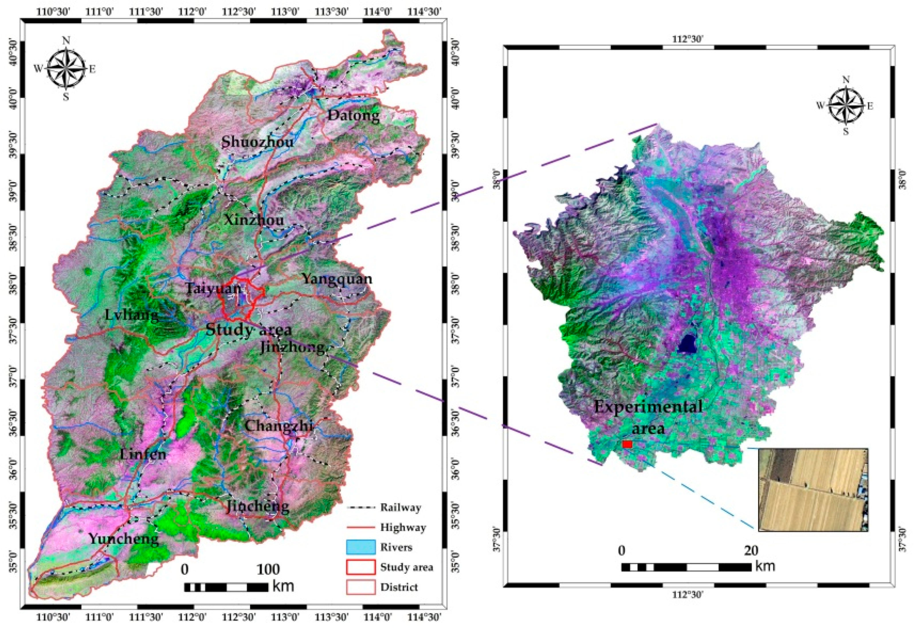
2.1. Study Area

The study area is located in Taiyuan City, Shanxi Province, China, specifically including Xiaodian District, Yingze District, Xinghualing District, Jiancaoping District, Wanbailin District, and Jinyuan District, with a total area of 1416 km² (Figure 1). It is the alluvial plain formed by Fenhe River, with a wide and flat terrain. Surrounded by mountains in the north, east, and west side, the elevation gradually decreases from north to south, with an average altitude of 800 m. It belongs to the semi-arid continental climate in the warm temperate zone, with the average annual temperature of 9.5 °C, the average annual wind speed of 2.5 m/s, the average annual precipitation of 483.5 mm, and the average annual evaporation of 1709.7 mm. A lot of cultivated lands are widely distributed in the study area. Three adjacent cultivated lands in the piedmont plain area of Jinyuan District were selected as the primary experimental area to extract cultivated land boundaries. Its geographical coordinates are located between 112°24′3.708″E and 112°24′20.198″E, 37°37′16.185″N and 37°37′25.723″N, with a coverage area of 0.12 km².

2.2. Data Sources

A GF-2 remote sensing image was used as the experimental data (

Table 1. Technical parameters of the GF-2 satellite.

Parameter	1 m Resolution Panchromatic/4 m Resolution Multispectral Camera
Spectral range	panchromatic	0.45–0.90 μm
	multispectral	0.45–0.52 μm
		0.52–0.59 μm
		0.63–0.69 μm
		0.77–0.89 μm
Spatial resolution	panchromatic	1 m
	multispectral	4 m
Width	45 km (Two cameras combined)
Revisit period	5 days

). It was obtained on 24 August 2015, with a spatial resolution of 1 m. A small subset of 400 × 300 pixels was randomly selected to extract cultivated land boundaries (Figure 2a). The image contrast enhancement was performed to show the edges of cultivated lands more clearly (Figure 2b). A larger GF-2 image acquired on 16 June 2015, with a subset size of 1000 × 1000 pixels, was used to validate the transferability of the proposed algorithm (Figure 2c). There were primary land cover types including cultivated land, village road, built-up area, and uncultivated land. The cultivated lands were fallow without the coverage of crops after harvesting the winter wheat. The data preprocessing procedures were first carried out including geometric correction, image fusion, and image cropping.

3. Methodology

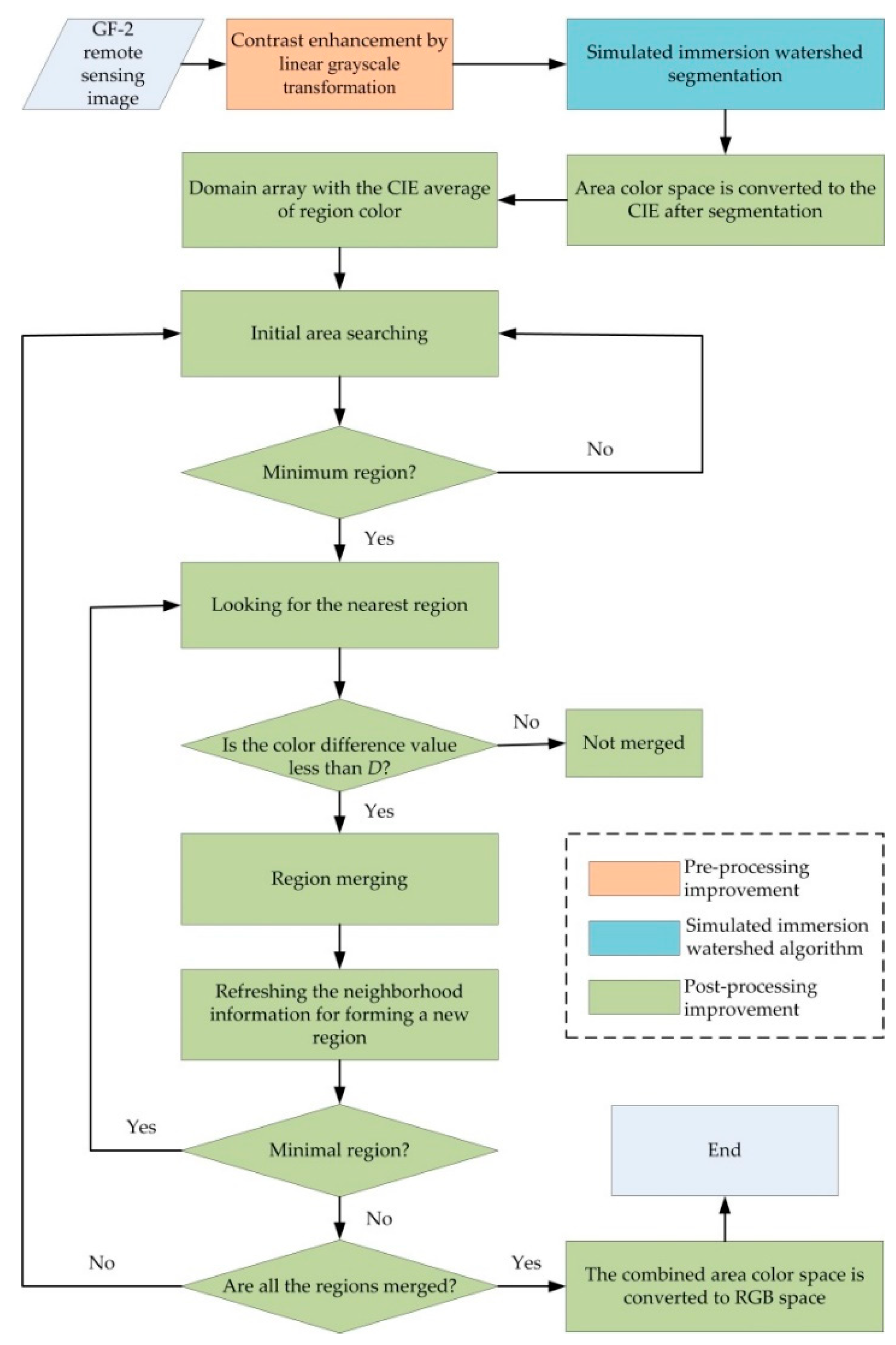
3.1. Technical Procedure

In comparison with RGB color space, the CIE color space is independent of the device, which is a better improvement for the color distance measurement. At present, some studies have adopted the Euclidean distance between two regions of CIE color space as the color difference to measure the color similarity. Better segmentation results are obtained by improving the regional similarity measure after finishing the watershed segmentation [34,35].

The improved algorithm was compared with the RGB color space-based algorithm. It involved in three major processes based on a combination of pre- and post-improvement procedures (Figure 3): (1) Pre-processing improvement module, which is image contrast enhancement; (2) post-processing improvement means that the color difference of CIE color space is used as the evaluation criterion for region merging; (3) evaluating the segmentation accuracy module, which include the δ_A, δ_P, and K_hat.

The image segmentation and merging experiments were performed on the CIE color space-based region merging watershed image segmentation system (hereafter referred to as CIE-WS). The system was developed based on the VC++, including three methods of RGB-RMWS, Lab-RMWS, and Luv-RMWS). The running time of image segmentation and merging experiments were respectively recorded using the CIE-WS’s built-in timing variable. All the experiments were operated by an Acer S40-51 computer with a 64-bit operating system, an Intel(R) Core(TM) i5-10210U CPU, a main frequency of 1.60 GHz, and an 8.00 GB memory.

3.2. Contrast Enhancement

Contrast enhancement is a kind of point operation on an image. The pixel value of the input image is converted to a new value through mapping transformation. The operation result will not change the spatial relationship between the pixels in the image, but can increase the contrast of the image and highlight the cultivated land information, which can improve the segmentation effect of the watershed algorithm based on spectral differences [34,35].

Linear grayscale transformation is one of the methods for contrast enhancement. This method assumes that the gray transformation range of the original image $f(x,y)$ is $[a,b]$, and that the gray transformation range of the processed image $g(x,y)$ is $[c,d]$. Linear expansion is carried out for the lowest and highest intensity data in the input image data. It can increase the dynamic range of the image, as well as can improve the image contrast of the clarity and features [36].

The $g(x,y)$ functions are shown in Equation (1):

$$g(x,y)=\{\begin{array}{c}d\\ \frac{d-c}{b-a}[f(x,y)-a]+c\\ c\end{array}\begin{array}{cc}& \begin{array}{ccc}& & \begin{array}{c}f(x,y)>b\\ a\le f(x,y)\le b\\ f(x,y)<a\end{array}\end{array}\end{array}$$

(1)

where a and b represent the gray transformation range of original image; c and d represent the gray transformation range of processed image.

After performing a set of trial-and-error experiments, [0.1, 0.9] is the optimal grayscale range for original image. The default value [0, 1] was used for processed image.

3.3. CIE Color Space and Transformation

3.3.1. Conversion between RGB and XYZ

CIE1976 specifies the RGB color space can be converted to the XYZ color space, and XYZ color space can be converted to the Lab or Luv color space. The color value of L, a, and b or L, u, and v can be obtained through the color space conversion from each channel of the image [37].

$$\left[\begin{array}{c}X\\ Y\\ Z\end{array}\right]=\left[\begin{array}{ccc}0.430& 0.342& 0.178\\ 0.222& 0.707& 0.071\\ 0.020& 0.130& 0.939\end{array}\right]\left[\begin{array}{c}R\\ G\\ B\end{array}\right]$$

(2)

$$L=\{\begin{array}{c}166\ast {(Y/Y_n)}^{1/3}-16\\ 903.3\ast \left(Y/Y_n\right)\end{array}\begin{array}{c}If\left(Y/Y_n\right)>0.008856\\ If\left(Y/Y_n\right)\le 0.008856\end{array}$$

(3)

where L is the brightness; X_n and Y_n are the tristimulus values of standard light source D65.

3.3.2. Color Space Conversion between XYZ and Lab

$$a=500\ast \left(f\left({X/X}_n\right)-f\left({Y/Y}_n\right)\right)$$

(4)

$$b=200\ast \left(f\left({Y/Y}_n\right)-f\left({Z/Z}_n\right)\right)$$

(5)

where a and b represent the chromaticity coordinates; Z_n is the tristimulus value of standard light source D65. X_n = 95.04, Y_n = 100.00, and Z_n = 208.88 [34].

The $f\left(t\right)$ functions in Equations (4) and (5) are shown in Equation (6):

$$f\left(t\right)=\{\begin{array}{c}{t}^{\frac{1}{3}} If t>0.008856\\ 7.787t+\frac{16}{116} If t\le 0.008856\end{array}$$

(6)

3.3.3. Color Space Conversion between XYZ and Luv

$$\{\begin{array}{c}u=13L\left(u^{\prime }-{u_n}^{\prime }\right)\\ v=13L\left(v^{\prime }-{v_n}^{\prime }\right)\end{array}$$

(7)

where u and v represent the chromaticity coordinates; ${u_n}^{\prime }$ and ${v_n}^{\prime }$ are the coordinates of the CIE standard light source and the tristimulus values given by [35]:

$$u^{\prime }=4X/\left(X+15Y+3Z\right)$$

(8)

$$v^{\prime }=9Y/\left(X+15Y+3Z\right)$$

(9)

$${u_n}^{\prime }=4X_n/\left(X_n+15Y_n+3Z_n\right)$$

(10)

$${v_n}^{\prime }=9Y_n/\left(X_n+15Y_n+3Z_n\right)$$

(11)

In the case of 2° observer and C light source, ${u_n}^{\prime }=0.2009$ and ${v_n}^{\prime }=0.4610$ [35]. 2° observer is the spectral tristimulus set by the CIE in 1931, also known as 1931 Standard Chroma Observer. CIE standard light sources include A, C, D50, D65, etc., and the C light source represents average daylight.

3.4. Watershed Segmentation Algorithm Based on CIE Color Space Region Merging

At present, the most widely used watershed algorithm is the simulated immersion algorithm, which was proposed by Vincent and Soille [38]. The steps of simulated immersion watershed algorithm are shown as follows [34]:

(1)

An image is converted from the color to corresponding grayscale.

(2)

The gradient of each pixel in the image is calculated. To sort the gradient values from smallest to largest, and the same gradient is located at the same gradient level.

(3)

To process all the pixels of the first gradient level and check the neighborhoods of a certain pixel. If the neighborhoods have already been identified as a certain area or watershed, add the pixel to a first-in first-out (FIFO) queue.

(4)

The first pixel would be picked up when the FIFO queue is not empty. To scan the pixel neighborhoods, the identification of pixel is refreshed according to the neighborhood pixel, when the gradient of its neighboring pixels belongs to the same layer. The loop will be continued just the same until the queue is empty.

(5)

To scan the pixel of current gradient level again, it will be a new minimal area if there are unidentified pixels. Continue to perform step (4) from this pixel until there is no new minimal region.

(6)

Return to step (3) to continue processing the next gradient level until all levels of pixels have been processed.

Many scholars have proposed different improved watershed segmentation algorithms according to their own research [34,35,39,40,41]. According to the watershed segmentation algorithm, these improved algorithms can be summarized as pre- and post- improvement, as well a combination of pre- and post-improvement for a traditional watershed segmentation algorithm.

In this study, on the basis of a simulated immersion algorithm, a combination of pre- and post-improvement procedures was used to improve the region merging watershed algorithm in CIE color space. More specifically, the contrast enhancement by linear grayscale transformation was used as the pre-improvement procedure, while the CIE color space region merging was used as the post-improvement procedure. The specific flowchart of the proposed algorithm can be found in Figure 4.

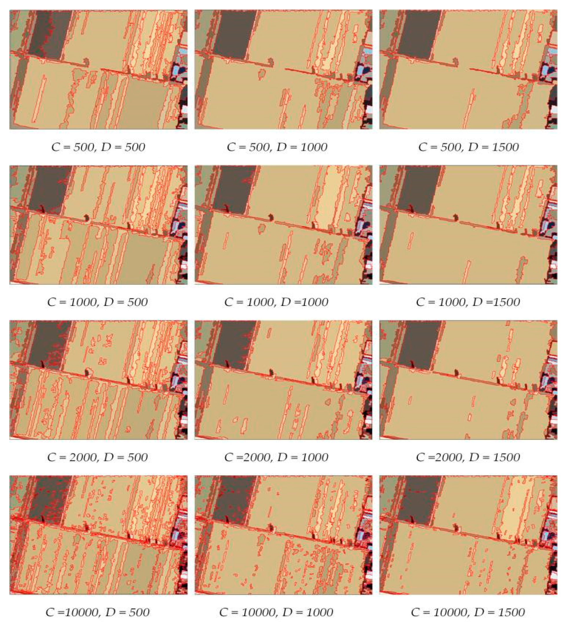
3.4.1. Segmentation Scale Parameter

The segmentation scale parameter by the watershed segmentation algorithm is the threshold value (A_min) of the minimal region. It is calculated by the following Equation [35]:

$$A_{\min }=(M\times N)/C$$

(12)

where M is the row of image; N is the column of image; C is a given constant. If a region is less than the A_min, it is a minimal region, otherwise it is not. The A_min depends on the value of C. Therefore, C value can be represented the segmentation scale parameters.

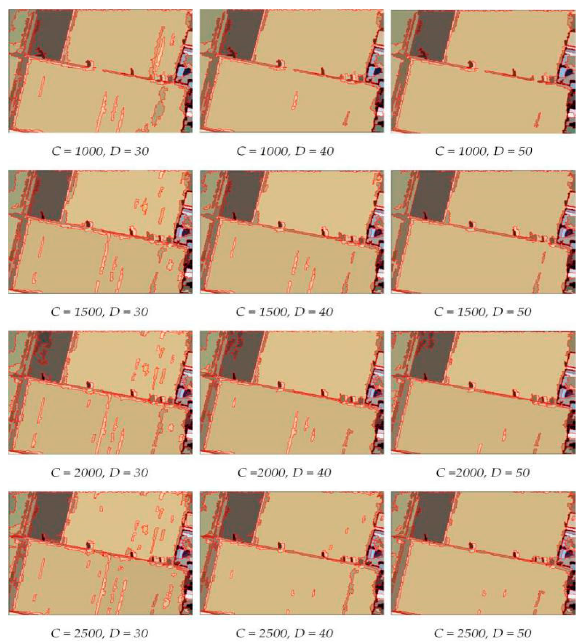
3.4.2. Merging Scale Parameters

In region merging after the watershed segmentation, how to determine the color similarity between two adjacent regions is the key problem. Here, the Euclidean distance ($d_i$) of two regions in the CIE color space was used as the color difference to measure the color similarity of two regions. It is calculated by the following Equation [35]:

$$d_i=\frac{\left|R_i\right|\cdot \left|R_j\right|}{\left|R_i\right|+\left|R_j\right|}\sqrt{{\displaystyle \sum _{\begin{array}{l}c=L,a,b\\ c=L,u,v\end{array}}{(F_c(R_i)-F_c(R_j))}^2}}\begin{array}{cc}& \end{array}i=1,2,3\cdot \cdot \cdot ,n;\begin{array}{cc}& \end{array}j=1,2,3\cdot \cdot \cdot ,n$$

(13)

where |R_i| and |R_j| are the pixel numbers contained in the image areas R_i and R_j, respectively; F_c(R_i) and F_c(R_j) are the average colors of image areas R_i and R_j; and n is the number of adjacent areas.

Let the merging threshold be D where $D={(d_i)}^2$. When $d_i\le \sqrt{D}$, the regions are merged; otherwise, the regions do not merge. Therefore, D can be used to represent the merging scale parameters. A smaller D corresponds to greater similarity between the colors, and vice versa.

As observed in Figure 4, the most critical technical problem of the watershed algorithm for region merging is to determine the minimum region and to merge similar regions, which are controlled by the segmentation threshold C values and the merging threshold D values, respectively [35]. At present, it is difficult to adaptively determine the C and D values. The trial-and-error procedure is usually used to conduct repetitive tests to find the optimal C and D values of the image information extraction.

4. Accuracy Evaluation of Image Segmentation

The segmentation quality of remote sensing image is a guarantee of the reliability of subsequent information analysis [42,43]. The way in which to evaluate the image segmentation results objectively and quantitatively is an important part of the image segmentation algorithm [44,45]. For the evaluation of image segmentation accuracy, many researchers have carried out qualitative and quantitative methods from different perspectives [46,47,48,49], and many evaluation methods and indicator systems have been proposed [50,51,52,53,54,55,56,57,58]. By comparing the evaluation, the segmentation accuracy of remote sensing images is indicated. On the basis of previous studies [34,35], the area relative error criterion (δ_A), the pixel quantity error criterion (δ_P), and the consistency criterion (K_hat) were selected to evaluate the segmentation accuracies. The reference data were obtained by visual interpretation or land use maps, and the segmentation results were obtained by the proposed method.

4.1. Area Relative Error Criterion (δ_A)

δ_A is the area relative error accuracy indicator. A₀ is the true area value of the target region in the benchmark image, and A_S is the area value of the target region in the segmentation result. It is calculated by the following equation [35]:

$${\delta }_A=\frac{|A_s-A_0|}{A_0}\times 100\%$$

(14)

A smaller δ_A corresponds to higher segmentation accuracy, and vice versa.

4.2. Pixel Quantity Error Criterion (δ_P)

δ_P is the pixel quantity error accuracy indicator. Let P_t is the correct number of pixels of the target region in the segmentation result, and P_w is the incorrect number. δ_P is calculated by the following equation [35]:

$${\delta }_P=\frac{P_w}{P_t+P_w}\times 100\%$$

(15)

A smaller δ_P corresponds to higher segmentation accuracy, and vice versa.

4.3. Consistency Criterion (K_hat)

K_hat is mainly used for accuracy evaluation and image consistency judgment. In this paper, K_hat was selected as the accuracy evaluation criterion for the consistency between the segmentation results and the benchmark data. Respectively, then, the K_hat is given by [59,60]:

$$K_{hat}=\frac{N{\displaystyle {\sum }_{i=1}^r{x}_{ii}-{\displaystyle {\sum }_{i=1}^r(x_{i+}{x}_{+i})}}}{N^2-{\displaystyle {\sum }_{i=1}^r(x_{i+}{x}_{+i})}}$$

(16)

where r represents the total number of columns in the error matrix; X_ii is the number of pixels in the row i and column i in the error matrix; x_i+ and x_+i are the total number of pixels in row i and column I, respectively; N is the total number of pixels used for accuracy evaluation.

The higher segmentation accuracy is indicated by a higher $K_{hat}$, and vice versa.

5. Results

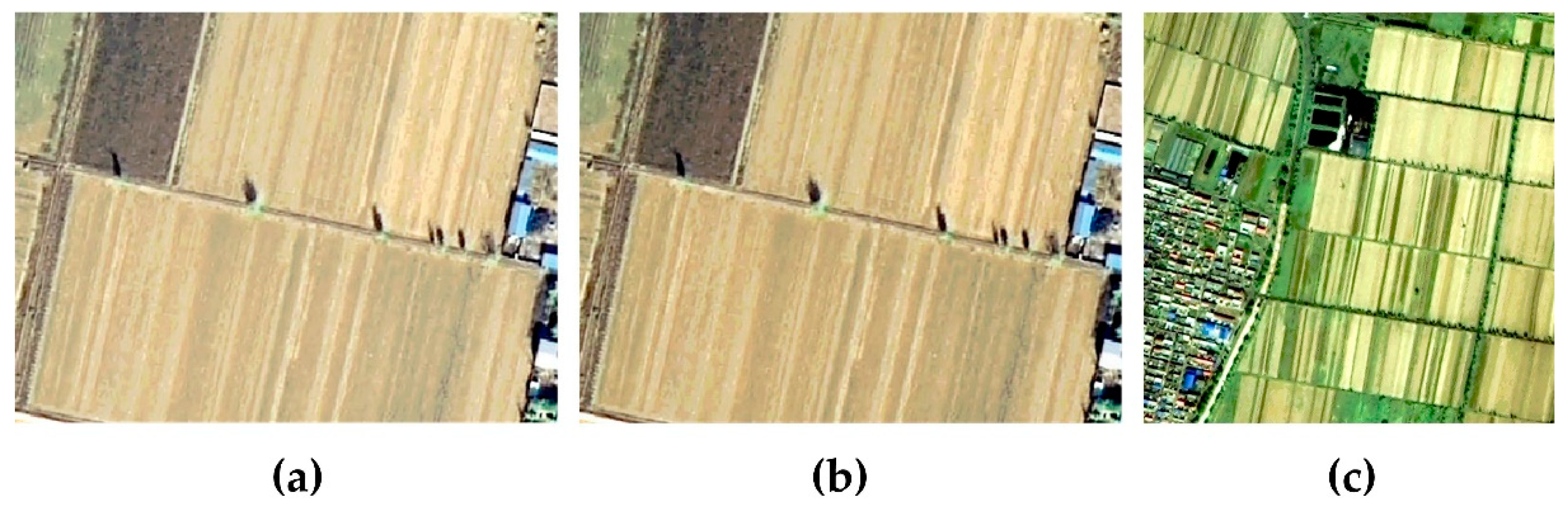
5.1. Image Segmentation before and after Contrast Enhancement

The segmented images were, respectively, obtained based on the pre- and post-contrast-enhanced image (Figure 5). To increase the comparability, the same C and D values were adopted in the experiments. The statistical results of the comparative experiments are provided in

Table 2. Statistical features derived from the three methods. RGB: Red–Green–Blue; RMWS: Region merging watershed segmentation.

Method	Experiment Image	Patch number of Simulated Immersion Algorithm	Time of Watershed Segmentation (s)	Number of Patches after Region Merging	Time of Area Merging (s)	C	D
RGB-RMWS	Original	14,389	0.063	133	4.578	2000	1000
	Contrast-enhanced	14,760	0.062	139	2.734	2000	1000
Lab-RMWS	Original	14,389	0.062	76	4.375	1900	40
	Contrast-enhanced	14,760	0.063	92	1.750	1900	40
Luv-RMWS	Original	14,389	0.062	91	2.125	2000	40
	Contrast-enhanced	14,760	0.063	117	1.906	2000	40

.

As observed in Figure 5, the blue boxes showed that the middle road of the cultivated land failed to maintain a continuous position in the segmentation results of Figure 5(a0,b0,c0). The corresponding positions remained continuous in Figure 5a–c. Meanwhile, Table 2 shows that the number of image spots in the contrast-enhanced image after segmentation and merging was higher than that in the original image. This can be also found by comparing the improvement of the road segmentation results in Figure 5. The contrast-enhanced image effectively avoided under-segmentation of the original image to the road. The results showed that contrast enhancement could improve the quality of image segmentation.

Table 2 shows that the initial image segmentation time was consistent. However, the time of the region merging varied greatly. The region merging time of the three methods was greatly reduced compared to that of the original image. The time efficiency of the contrast-enhanced image segmentation and merging in the Lab-RMWS method was 60.00% higher than that of original images. The Luv-RMWS and RGB-RMWS methods were improved by 10.31% and 40.28%, respectively. Therefore, contrast enhancement could improve the time efficiency of region merging watershed segmentation.

5.2. The Optimal Scale Parameters in the Three Methods

The optimal segmentation and merging scale parameters are the C and D values in the three watershed segmentation methods. The trial-and-error multiscale segmentation experiments were performed on the test contrast-enhanced images with the combinations of different C and D values.

(1) Multiscale segmentation experiments of RGB-RMWS

The C and D values varied between 100 and 15,000 at intervals of 50. Some important segmentation results are shown in Figure 6.

(2) Multiscale segmentation experiments of Lab-RMWS

The C value varied between 100 and 5000 at intervals of 50, and the D value varied between 10 and 500 at intervals of 10. Some important segmentation results are shown in Figure 7.

(3) Multiscale segmentation experiments of Luv-RMWS

The C value varied between 100 and 5000 at intervals of 50, and the D value varied between 10 and 500 at intervals of 10. Some important segmentation results are shown in Figure 8.

The statistical results of the combinations of different C and D values are provided in

Table 3. Statistical features derived from the combinations of different C and D values.

Experiment Image	Method	Number of Sliver Polygons after Region Merging	C	D
Contrast-enhanced	RGB-RMWS	38	100	100
		3	100	15,000
		2421	15,000	100
		44	15,000	15,000
	Lab-RMWS	20	100	10
		4	100	500
		524	5000	10
		58	5000	500
	Luv-RMWS	26	100	10
		4	100	500
		655	5000	10
		56	5000	500

.

As observed from Figure 6, Figure 7 and Figure 8 and Table 3, with the gradual increase in C values, the number of sliver polygons in the image segmentation results increased, and the image tended to be over-segmented. As the D values gradually increased, the number of sliver polygons decreased and the image tended to be under-segmented. Thus, a bivariate orthogonal scale parameter space was formed. The image to be segmented achieved the optimal segmentation result when the C and D values obtained a certain scale. The multiscale segmentation experiments show that the optimal C values are equal to 2000 and the D values are equal to 1000 in the RGB-RMWS method, while the optimal C values are equal to 1900 and the D values are equal to 40 in the Lab-RMWS method, and the optimal C values are equal to 2000 and the D values are equal to 40 in the Luv-RMWS method.

5.3. Extraction of Cultivated Land Boundaries

The reference data of the cultivated land boundaries in the experimental area were obtained by visual interpretation, and the optimal C and D values of the three methods were obtained by experiment. The segmentation results were taken as the results of the cultivated land boundary extraction. To compare the extraction effect derived from the three methods, the optimal experimental results, benchmark data, and experimental images are overlaid and displayed (Figure 9).

As shown in Figure 9, there are some sliver polygons on the edge of and in the cultivated lands, and they are 28, 9, and 14, respectively, for the three methods. Therefore, the Lab-RMWS method was the best of the three methods. Its cultivated land boundary provided the best result. On the contrary, the RGB-RMWS method results were worst. It is obvious that there were many sliver polygons in cultivated lands. The post-processing was implemented by manual intervention. Some additional time was required to merge them. It is observed from Figure 9b,c that the Lab-RMWS and Luv-RMWS methods not only extract better cultivated land boundaries, but also merge sliver polygons in the cultivated land. Both the cultivated land boundaries and road in the cultivated land are continuous and complete. The extracted cultivated land boundaries are rarely affected by vegetation, trees, roads, bare areas, and constructions. The segmentation results are better than the RGB-RMWS method. However, as shown in Figure 9b,c, some over- and under-segmentation phenomena still exist. There were still segmented patches all around and inside the cultivated land, and the patches of trees along the middle road were attached and mis-divided, affecting the overall extraction effect.

5.4. Running Time of Segmentation Experiments

To compare the running time of the three methods during segmentation experiments, the statistical results are provided in

Table 4. Comparison of the running time of the segmentation experiments.

Method	Running Time (s)	C	D	Note
RGB-RMWS	2.796	2000	1000	All the three methods can perform automatic image segmentation and merging.
Lab-RMWS	1.813	1900	40
Luv-RMWS	1.969	2000	40

.

Table 4 shows that the RGB-RMWS, Lab-RMWS, and Luv-RMWS methods all had higher time efficiencies. Among them, the RGB-RMWS method used the most time of 2.796 s. Meanwhile, the Lab-RMWS and Luv-RMWS methods had similar time efficiencies, which were 1.813 s and 1.969 s, respectively. These results are better than those of the RGB-RMWS method without improving the color space. Meanwhile, the time efficiency of the Lab-RMWS and Luv-RMWS methods were improved by 35.16% and 29.58%, respectively, compared to the RGB-RMWS method.

5.5. Extraction Accuracy

The proposed method was compared with the RGB-RMWS. For fair comparison, the same accuracy evaluation factors were adopted by all comparison methods. For each method, the result of δ_A, δ_P, and K_hat can be found in

Table 5. Evaluation of the accuracy of the cultivated land extraction from the experimental images.

Criterion	Indicator	RGB-RMWS	Lab-RMWS	Luv-RMWS
Area relative error	δA	10.27%	2.37%	4.54%
Pixel quantity error	δP	9.16%	3.48%	4.61%
Consistency	Khat	77.86%	90.96%	88.31%

.

Table 5 shows that both the Lab-RMWS and Luv-RMWS methods had higher image segmentation precision. All the δ_A, δ_P, and K_hat were superior to the RGB-RMWS method without improving the color space. The δ_A, δ_P, and K_hat of the Lab-RMWS method were 2.37%, 3.48%, and 90.96%, respectively, which are superior to those of the Luv-RMWS method. The Lab-RMWS method was the most accurate segmentation method among the three methods. The δ_A, δ_P, and K_hat of the Lab-RMWS method were 76.92%, 62.01%, and 16.83%, respectively, higher than those of the RGB-RMWS method. The δ_A, δ_P, and K_hat of the Luv-RMWS method were 55.79%, 49.67%, and 13.42%, respectively, higher than those of the RGB-RMWS method.

5.6. Comparison Experiment with a Larger Image

To test the transferability of the proposed method to another type of parcel, a larger image was used to perform the comparison experiment. To increase the comparability, the same optimal C and D values were adopted in the experiments. The segmented images were obtained based on the contrast-enhanced image of Figure 2c. The reference data of cultivated land boundaries were derived from visual interpretation (Figure 10). The statistics of the comparison experiments are provided in

Table 6. Statistics of the comparison experiment derived from the three methods.

Method	Number of Sliver Polygons Using the Simulated Immersion Algorithm	Time of Watershed Segmentation (s)	Number of Sliver Polygons after Region Merging	Time of Region Merging (s)	C	D
RGB-RMWS	53,710	0.687	318	14.961	2000	1000
Lab-RMWS	53,710	0.687	316	8.252	1900	40
Luv-RMWS	53,710	0.687	378	8.908	2000	40

.

It could be found that the segmentation results of 7, 8, 11, and 12 cultivated lands were better, with higher integrity, continuous boundaries, and less silver polygons. Conversely, they were bad for other cultivated lands with a lot of sliver polygons. In comparison with Figure 2c, it can be seen that the internal homogeneity of 7, 8, 11, and 12 cultivated lands are higher, while the internal heterogeneity of other cultivated lands is higher. It is obvious that the segmentation effect is significantly affected by the internal homogeneity and heterogeneity of cultivated lands. As shown in Figure 10 and Table 6, Lab-RMWS had the best performance among the three methods. On the contrary, RGB-RMWS-based segmentation results were the worst. There were some sliver polygons in cultivated lands by the three methods to a certain degree. The post-processing was implemented by manual intervention, so additional time was required to merge them.

For each method, the quantitative evaluation indicators could be found in

Table 7. Evaluation of the accuracies using the three methods.

Criterion	Indicator	RGB-RMWS	Lab-RMWS	Luv-RMWS
Area relative error	δA	14.09%	5.15%	7.55%
Pixel quantity error	δP	9.71%	4.44%	6.20%
Consistency	Khat	80.12%	90.62%	86.99%

. It showed that both the Lab-RMWS and Luv-RMWS methods had higher image segmentation precision, and all the δ_A, δ_P, and K_hat were superior to the RGB-RMWS method. The improved algorithm based on the Lab color space performed better than the improved algorithm based on the Luv color space.

6. Discussion

6.1. Analysis of the Contrast Enhancement Image Segmentation

As shown in Figure 5 and Table 2, contrast enhancement could improve the image segmentation quality and the image segmentation time efficiency. It is an effective technique to improve the pre-processing of the watershed algorithm. At present, there are many methods for image enhancement [61,62]. In the future, comparative experiments on various image enhancement methods should be carried out. The best image enhancement method should be selected to assist the improvement of the CIE color space region merging watershed algorithm in order to improve the image segmentation quality and time efficiency.

6.2. Analysis of the Optimal Scale Parameters

The optimal scale parameter selection of the region merging watershed algorithm mainly refers to the selection of the C value and D value [35]. In this paper, a GF-2 remote sensing image has been used to conduct the optimal scale parameter selection trial-and-error experiment on the improved algorithm. The performed experiments showed that the optimal C values of the RGB-RMWS, Lab-RMWS, and Luv-RMWS methods were 2000, 1900, and 2000, while the optimal D values were 1000, 40, and 40, respectively. However, the optimal scale parameters of the three color space region merging watershed algorithms obtained in this study were mainly based on the experiment to obtain the empirical optimal values. It was subjective to a certain extent, and was greatly affected by the image texture, tone, time phase, image contrast enhancement method, etc. Subsequent studies still need to continue to explore the objective acquisition method of the optimal scale parameters.

6.3. Analysis of the Extraction Effect

Optimal segmentation results should satisfy the following conditions: (1) The cultivated land boundary is continuous and complete; (2) the road in the cultivated land is continuous and complete; (3) the cultivated land map’s internal sliver polygons are as little as possible. Nowadays, the subjective evaluation method is still the most commonly used for evaluation of the segmentation effect [45]. Compared to the original RGB color space, the improved CIE color space watershed algorithm obviously improved the visual comparison of the segmentation results. At the same time, the cultivated land boundaries were divided completely, and less sliver polygons remained in the cultivated land. The basic principle of greater homogeneity in the image spot after segmentation was achieved. A comparison of the accuracy evaluation showed that the improved watershed algorithm of the CIE color space was more accurate than that of the RGB color space. At the same time, Table 5 and Table 7 shows that the evaluation indicators of δ_A, δ_P, and K_hat had better consistency in the accuracy evaluation of the three methods. These evaluation indicators are an effective combination of precision evaluation indicators of the watershed segmentation algorithm.

6.4. Analysis of the Proposed Method

At present, there is much research on extracting cultivated land boundaries based on remote sensing images [7]. The types of data used for research are varied. The extraction method has gradually transformed from unsupervised [20] and supervised classification [21] with poor effects to support vector machines [19], object-oriented classification [23], random forests [27], neural networks [28], and deep learning [31] with good effects. However, these methods, inevitably, have problems such as complex rules and inadequate applicability. The principle of the watershed algorithm is simple, and the processing process is highly automated, and some attempts have been made in the field of boundary extraction [13,32]. Based on Lab, the Luv color space watershed algorithm is an improved algorithm for region merging in the CIE color space. This improved algorithm has achieved better results in slope hazard boundary extraction [34,35].

In this study, a GF-2 remote sensing image from China was selected. The pre-processing was improved by the enhancement of linear gray scale transformation, while the CIE color space region merging improved the post-processing. The simulated immersion algorithm was improved by combining the "pre + post" improvements. Compared to the original RGB color space region merging watershed algorithm, cultivated land boundary extraction was studied and tested. The δ_A, δ_P, and K_hat was used to construct the segmentation accuracy evaluation indicators combined as evaluation indicators. The comparison experiments showed that the improved algorithm in this study is superior to the unimproved algorithm in terms of the visual comparison, time efficiency, and extraction precision of cultivated land boundaries. The improved algorithm based on the Lab color space performed better than the improved algorithm based on the Luv color space. At the same time, the indicators of δ_A, δ_P, and K_hat had high consistency in the accuracy evaluation. The accuracy evaluation results were completely consistent with that of visual results of accuracy evaluation. The study provides an objective and reliable combination of indicators for improving the accuracy evaluation of the watershed segmentation algorithm.

7. Conclusions

An improved watershed algorithm system based on "pre + post" processing was proposed for cultivated land boundary extraction. Its includes image contrast enhancement, CIE color space region merging, and segmentation accuracy evaluation criteria based on the area relative error criterion, the pixel quantity error criterion, and the consistency criterion. The experimental results showed that the improved CIE color space region merging watershed algorithm is superior to the unimproved RGB color space region merging watershed algorithm in terms of visual effect, time efficiency, and extraction accuracy. The time efficiency has been improved in the Lab and Luv color spaces by 35.16% and 29.58%, respectively. The δ_A, δ_P, and K_hat indicators were improved by 76.92%, 62.01%, and 16.83% in the Lab color space, respectively, and 55.79%, 49.67%, and 13.42% in the Luv color space. The evaluation results of the three accuracy indicators were consistent. The comparison experiments based on a larger image are still consistent with the small image, showing that the proposed method has satisfying segmentation performance and transferability. The proposed method is easier to be understood than other methods, and the image processing of segmentation and region merging is simple. Its time efficiency and result accuracy perform well, and the degree of automation is higher. It has a certain reference value for the selection of a cultivated land boundary extraction method of high-resolution remote sensing images. Furthermore, it extends the application field of the watershed segmentation algorithm.

References

1. Useya, J.; Chen, S.B. Exploring the potential of mapping patterns on small holder scale croplands using Sentinel-1 SAR Data. Chin. Geogr. Sci. 2019, 29, 626–639. [Google Scholar] [CrossRef] [Green Version]
2. Chen, G.; Sui, X.; Kamruzzaman, M.M. Agricultural Remote Sensing Image Cultivated Land Extraction Technology Based on Deep Learning. Rev. Tecn. Fac. Ingr. Univ. Zulia. 2019, 36, 2199–2209. [Google Scholar]
3. Ma, E.P.; Cai, J.M.; Lin, J.; Guo, H.; Han, Y.; Liao, L.W. Spatio-temporal evolution of global food security pattern and its influencing factors in 2000–2014. Acta Geol. Sin. 2020, 75, 332–347. [Google Scholar]
4. Deng, J.S.; Wang, K.; Shen, Z.Q.; Xu, H.W. Decision tree algorithm for automatically extracting farmland information from SPOT-5 images based on characteristic bands. Trans. CSAET 2004, 20, 145–148. [Google Scholar]
5. Fritz, S.; See, L.; Mccallum, I.; Bun, A.; Moltchanova, E.; Duerauer, M.; Perger, C.; Havlik, P.; Mosnier, A.; Schepaschenko, D. Mapping global cropland and field size. Glob. Chang. Biol. 2015, 21, 1980–1992. [Google Scholar] [CrossRef]
6. Dimov, D.; Low, F.; Ibrakhimov, M.; Schonbrodt-Stitt, S.; Conradl, C. Feature extraction and machine learning for the classification of active cropland in the Aral Sea Basin. In Proceedings of the 2017 IEEE International Geoscience and Remote Sensing Symposium (IGARSS), Fort Worth, TX, USA, 23–28 July 2017; pp. 1804–1807. [Google Scholar]
7. Xiong, X.L.; Hu, Y.M.; Wen, N.; Liu, L.; Xie, J.W.; Lei, F.; Xiao, L.; Tang, T. Progress and prospect of cultivated land extraction research using remote sensing. J. Agric. Resour. Environ. 2020, 37, 856–865. [Google Scholar]
8. Zhao, G.X.; Dou, Y.X.; Tian, W.X.; Zhang, Y.H. Study on automatic abstraction methods of cultivated land information from satellite remote sensing images. Geographic Sinica 2001, 21, 224–229. [Google Scholar]
9. Tan, C.P.; Ewe, H.T.; Chuah, H.T. Agricultural crop-type classification of multi-polarization SAR images using a hybrid entropy decomposition and support vector machine technique. Int. J. Remote Sens. 2011, 32, 7057–7071. [Google Scholar] [CrossRef]
10. Xu, P.; Xu, W.C.; Luo, Y.F.; Zhao, Z.X. Precise classification of cultivated land based on visible remote sensing image of UAV. J. Agric. Sci. Technol. 2019, 21, 79–86. [Google Scholar]
11. Inglada, J.; Michel, J. Qualitative spatial reasoning for high resolution remote sensing image analysis. IEEE Trans. Geosci. Remote Sens. 2009, 47, 599–612. [Google Scholar] [CrossRef]
12. Blaschke, T.; Hay, G.J.; Kelly, M.; Lang, S.; Hofmann, P.; Addink, E.; Feitosa, R.Q.; Van der Meer, F.; Van der Werff, H.; Van Coillie, F.; et al. Geographic Object-Based Image Analysis-Towards a new paradigm. ISPRS J. Photogramm. 2014, 87, 180–191. [Google Scholar] [CrossRef] [PubMed] [Green Version]
13. Zhou, W.; Ming, D.P.; Yan, P.F. Cultivated Land Extraction Based on Image Region Division and Scale Estimation. J. Geo-Inf. Sci. 2018, 20, 1014–1025. [Google Scholar]
14. Wu, Z.T.; Thenkabail, P.S.; Mueller, R.; Zakzeski, A.; Melton, F.; Johnson, L.; Rosevelt, C.; Dwyer, J.; Jones, J.; Verdin, J.P. Seasonal cultivated and fallow cropland mapping using the MODIS-based automated cropland classification algorithm. J. Appl. Remote Sens. 2014, 8, 397–398. [Google Scholar] [CrossRef] [Green Version]
15. Xiong, J.; Thenkabail, P.S.; Gumma, M.K.; Teluguntla, P.; Poehnelt, J.; Congalton, R.G.; Yadav, K.; Thau, D. Automated cropland mapping of continental Africa using Google Earth Engine cloud computing. ISPRS J. Photogramm. 2017, 126, 225–244. [Google Scholar] [CrossRef] [Green Version]
16. Graesser, J.; Ramankutty, N. Detection of cropland field parcels from Landsat imagery. Remote Sens. Environ. 2017, 201, 165–180. [Google Scholar] [CrossRef] [Green Version]
17. Belgiu, M.; Csillik, O. Sentinel-2 cropland mapping using pixel-based and object-based time-weighted dynamic time warping analysis. Remote Sens. Environ. 2018, 204, 509–523. [Google Scholar] [CrossRef]
18. Li, S.H.; Jin, B.X.; Zhou, J.S.; Wang, J.L.; Peng, S.Y. Analysis of the spatiotemporal land-use/land-cover change and its driving forces in Fuxian Lake Watershed, 1974 to 2014. Pol. J. Environ. Stud. 2017, 26, 671–681. [Google Scholar] [CrossRef]
19. Li, C.J.; Huang, H.; Li, W. Research on agricultural remote sensing image cultivated land extraction technology based on support vector. Instrum. Technol. 2018, 11, 5-8+48. [Google Scholar]
20. Zhang, Y.H.; Zhao, G.X. The Research on Farm Land Information Secondary Planet Remote Sensing Computer Automatic Extraction Techniques Using the ENVI Software. J. Sichuan Agric. Univ. 2000, 18, 170–172. [Google Scholar]
21. NNiu, L.Y.; Zhang, X.Y.; Zheng, J.Y.; Cao, S.D.; Ruan, H.J. Extraction of Cultivated Land Information in Shandong Province Based on Landsat8 OLI Data. Chin. Agric. Sci. Bull. 2014, 30, 264–269. [Google Scholar]
22. Xiao, G.F.; Zhu, X.F.; Hou, C.Y.; Xia, X.S. Extraction and analysis of abandoned farmland: A case study of Qingyun and Wudi counties in Shandong Province. Acta Geogr. Sin. 2018, 73, 1658–1673. [Google Scholar] [CrossRef] [Green Version]
23. Mu, Y.X.; Wu, M.Q.; Niu, Z.; Huang, W.J.; Yang, J. Method of remote sensing extraction of cultivated land area under complex conditions in southern region. Remote Sens. Technol. Appl. 2020, 35, 1127–1135. [Google Scholar]
24. Bouziani, M.; Goita, K.; He, D.C. Rule-based classification of a very high resolution image in an urban environment using multispectral segmentation guided by cartographic data. IEEE Trans. Geosci. Remote 2010, 48, 3198–3211. [Google Scholar] [CrossRef]
25. Chen, J.; Chen, T.Q.; Liu, H.M.; Mei, X.M.; Shao, Q.B.; Deng, M. Hierarchical extraction of farmland from high-resolution remote sensing imagery. Trans. Chin. Soc. Agric. Eng. 2015, 31, 190–198. [Google Scholar]
26. Li, P.; Yu, H.; Wang, P.; Li, K.Y. Comparison and analysis of agricultural information extraction methods based on GF2 satellite images. Bull. Surv. Mapp. 2017, 1, 48–52. [Google Scholar]
27. Teluguntla, P.; Thenkabail, P.S.; Oliphant, A.; Xiong, J.; Gumma, M.K.; Congalton, R.G.; Yadav, K.; Huete, A. A 30-m landsat-derived cropland extent product of Australia and China using a random forest machine learning algorithm on Google Earth Engine cloud computing platform. ISPRS J. Photogramm. 2018, 144, 325–340. [Google Scholar] [CrossRef]
28. Yang, Z.J.; Chen, X.; Yang, L.; Wang, W.S.; Cao, Q. Extraction method of cultivated land information based on remote sensing time series spectral reconstruction. Sci. Surv. Mapp. 2020, 45, 59–67. [Google Scholar]
29. Zhou, X.; Wang, Y.B.; Liu, S.H.; Yu, P.X.; Wang, X.K. A machine learning algorithm for automatic identification of cultivated land in remote sensing images. Remote Sens. Land Res. 2018, 30, 68–73. [Google Scholar]
30. Tian, L.J.; Song, W.L.; Lu, Y.Z.; Lü, J.; Li, H.X.; Chen, J. Rapid monitoring and classification of land use in agricultural areas by UAV based on the deep learning method. J. China Ins. W. Res. Hydropower Res. 2019, 17, 312–320. [Google Scholar]
31. Li, S.; Peng, L.; Hu, Y.; Chi, T.H. FD-RCF -based boundary delineation of agricultural fields in high resolution remote sensing images. J. Univ. Chin. Acad. Sci. 2020, 37, 483–489. [Google Scholar]
32. Hu, T.G.; Zhu, W.Q.; Yang, X.Q.; Pan, Y.Z.; Zhang, J.S. Farmland Parcel Extraction Based on High Resolution Remote Sensing Image. Spectrosc. Spect. Anal. 2009, 29, 2703–2707. [Google Scholar]
33. Hu, X.; Li, X.J. Comparison of subsided cultivated land extraction methods in high-ground water-level coal mines based on unmanned aerial vehicle. J. China Coal Soc. 2019, 44, 3547–3555. [Google Scholar]
34. Zhang, M.M.; Ge, Y.H.; Xue, Y.A.; Zhao, J.L. Identification of geomorphological hazards in an underground coal mining area based on an improved region merging watershed algorithm. Arab. J. Geosci. 2020, 13, 339. [Google Scholar] [CrossRef]
35. Zhang, M.M.; Xue, Y.A.; Ge, Y.H.; Zhao, J.L. Watershed segmentation algorithm based on Luv color space region merging for extracting slope hazard boundaries. ISPRS Int. J. Geo-Inf. 2020, 9, 246. [Google Scholar] [CrossRef]
36. Gai, J.D.; Ding, J.X.; Wang, D.; Xiao, Q.; Deng, J. Study on Extracting the Gearing Mesh Mark and Tooth Profile of Hypoid Gear based on Linear Gray Scale Transformation. J. Mech. Tx. 2011, 35, 27–30. [Google Scholar]
37. Lin, F.Z. Foundation of Multimedia Technology, 3rd ed.; Tsinghua University Press: Beijing, China, 2009; pp. 104–106. [Google Scholar]
38. Vincent, L.; Soille, P. Watersheds in digital spaces: An efficient algorithm based on immersion simulations. Comput. Archit. Lett. 1991, 13, 583–598. [Google Scholar] [CrossRef] [Green Version]
39. Li, B.; Pan, M.; Wu, Z.X. An improved segmentation of high spatial resolution remote sensing image using marker-based watershed algorithm. In Proceedings of the 20th International Conference on Geoinformatics, Hong Kong, China, 15–17 June 2012. [Google Scholar]
40. Wang, Y. Adaptive marked watershed segmentation algorithm for red blood cell images. J. Image Graph. 2018, 22, 1779–1787. [Google Scholar]
41. Jia, X.Y.; Jia, Z.H.; Wei, Y.M.; Liu, L.Z. Watershed segmentation by gradient hierarchical reconstruction under opponent color space. Comput. Sci. 2018, 45, 212–217. [Google Scholar]
42. Yasnoff, W.A.; Mui, J.K.; Bacus, J.W. Error measures for scene segmentation. Pattern Recogn. 1977, 9, 217–231. [Google Scholar] [CrossRef]
43. Dorren, L.K.A.; Maier, B.; Seijmonsbergen, A.C. Improved Landsat-based forest mapping in steep mountainous terrain using object-based classification. For. Ecol. Manag. 2003, 183, 31–46. [Google Scholar] [CrossRef]
44. Ming, D.P.; Luo, J.C.; Zhou, C.H.; Wang, J. Research on high resolution remote sensing image segmentation methods based on features and evaluation of algorithms. Geo-Inform. Sci. 2006, 8, 107–113. [Google Scholar]
45. Chen, Y.Y.; Ming, D.P.; Xu, L.; Zhao, L. An overview of quantitative experimental methods for segmentation evaluation of high spatial remote sensing images. J. Geo-Inform. Sci. 2017, 19, 818–830. [Google Scholar]
46. Huang, Q.; Dom, B. Quantitative methods of evaluating image segmentation. In Proceedings of the International Conference on Image Processing, Washington, DC, USA, 23–26 October 1995. [Google Scholar]
47. Jozdani, S.; Chen, D.M. On the versatility of popular and recently proposed supervised evaluation metrics for segmentation quality of remotely sensed images: An experimental case study of building extraction. ISPRS J. Photogramm. 2020, 160, 275–290. [Google Scholar] [CrossRef]
48. Debelee, T.G.; Schwenker, F.; Rahimeto, S.; Yohannes, D. Evaluation of modified adaptive k-means segmentation algorithm. Comput. Vis. Media 2019, 5, 347–361. [Google Scholar] [CrossRef] [Green Version]
49. Zhang, H.; Fritts, J.E.; Goldman, S.A. Image segmentation evaluation: A survey of unsupervised methods. Comput. Vis. Image Underst. 2008, 110, 260–280. [Google Scholar] [CrossRef] [Green Version]
50. Zhu, C.J.; Yang, S.Z.; Cui, S.C.; Cheng, W.; Cheng, C. Accuracy evaluating method for object-based segmentation of high resolution remote sensing image. High. Power Laser Part Beams 2015, 27, 37–43. [Google Scholar]
51. Hoover, A.; Jean-Baptiste, G.; Jiang, X.Y.; Flynn, P.J.; Bunke, H.; Goldgof, D.; Bowyer, K.; Eggert, D.W.; Fitzgibbon, A.; Fisher, R. An experimental comparison of range image segmentation algorithms. IEEE Trans. Pattern Anal. Mach. Intell. 1996, 18, 673–689. [Google Scholar] [CrossRef] [Green Version]
52. Chen, H.C.; Wang, S.J. The use of visible color difference in the quantitative evaluation of color image segmentation. In Proceedings of the IEEE International Conference on Acoustics, Speech, and Signal Processing, Montreal, QC, Canada, 17–21 May 2004. [Google Scholar]
53. Hay, G.J.; Castilla, G.; Wulder, M.A.; Ruiz, J.R. An automated object-based approach for the multiscale image segmentation of forest scenes. Int. J. Appl. Earth Observ. 2005, 7, 339–359. [Google Scholar] [CrossRef]
54. Cardoso, J.S.; Corte-Real, L. Toward a generic evaluation of image segmentation. IEEE Trans. Image Process. 2005, 14, 1773–1782. [Google Scholar] [CrossRef] [PubMed] [Green Version]
55. Hofmann, P.; Lettmayer, P.; Blaschke, T.; Belgiu, M.; Wegenkittl, S.; Graf, R.; Lampoltshammer, T.J.; Andrejchenko, V. Towards a framework for agent-based image analysis of remote-sensing data. Int. J. Image Data Fusion 2015, 6, 115–137. [Google Scholar] [CrossRef] [Green Version]
56. Zhang, X.L.; Feng, X.Z.; Xiao, P.F.; He, G.J.; Zhu, L.J. Segmentation quality evaluation using region-based precision and recall measures for remote sensing images. ISPRS J. Photogramm. 2015, 102, 73–84. [Google Scholar] [CrossRef]
57. Wei, X.W.; Zhang, X.F.; Xue, Y. Remote sensing image segmentation quality assessment based on spectrum and shape. J. Geo-Inform. Sci. 2018, 20, 1489–1499. [Google Scholar]
58. Li, Z.Y.; Ming, D.P.; Fan, Y.L.; Zhao, L.F.; Liu, S.M. Comparison of evaluation indexes for supervised segmentation of remote sensing imagery. J. Geo-Inform. Sci. 2019, 21, 1265–1274. [Google Scholar]
59. Huang, T.; Bai, X.F.; Zhuang, Q.F.; Xu, J.H. Research on Landslides Extraction Based on the Wenchuan Earthquake in GF-1 Remote Sensing Image. Bull. Surv. Mapp. 2018, 2, 67–71. [Google Scholar]
60. Li, Q.; Zhang, J.F.; Luo, Y.; Jiao, Q.S. Recognition of earthquake-induced landslide and spatial distribution patterns triggered by the Jiuzhaigou earthquake in August 8, 2017. J. Remote Sens. 2019, 23, 785–795. [Google Scholar]
61. Samarasinha, N.H.; Larson, S.M. Image enhancement techniques for quantitative investigations of morphological features in cometary comae: A comparative study. Icarus 2014, 239, 168–185. [Google Scholar] [CrossRef] [Green Version]
62. Alberto, L.C.; Erik, C.; Marco, P.C.; Fernando, F.; Arturo, V.G.; Ram, S. Moth Swarm Algorithm for Image Contrast Enhancement. Knowl-Based Syst. 2020, 212, 106607. [Google Scholar]
Figure 1. Geographical location of the study area.
Remotesensing 13 00939 g001
Figure 2. A subset of Gaofen-2 (GF-2) remote sensing images: (a) Original small image, (b) contrast-enhanced small image, and (c) larger image.
Remotesensing 13 00939 g002
Figure 3. The flowchart of the improved method in this study.
Remotesensing 13 00939 g003
Figure 4. Flowchart of the watershed segmentation algorithm based on Commission Internationale de l´Eclairage (CIE) color space region merging.
Remotesensing 13 00939 g004
Figure 5. Comparison of segmentation results between the pre- and post-contrast-enhanced images.
Remotesensing 13 00939 g005
Figure 6. Some important segmentation results of cultivated land boundaries using the RGB-RMWS.
Remotesensing 13 00939 g006
Figure 7. Some important segmentation results of cultivated land boundaries using the Lab-RMWS.
Remotesensing 13 00939 g007
Figure 8. Some important segmentation results of cultivated land boundaries using the Luv-RMWS.
Remotesensing 13 00939 g008
Figure 9. Comparison of the optimal extracted cultivated land boundary using the three methods: (a) RGB-RMWS; (b) Lab-RMWS; (c) Luv-RMWS.
Remotesensing 13 00939 g009
Figure 10. Comparison of the extracted cultivated land boundaries using (a) RGB-RMWS, (b) Lab-RMWS, and (c) Luv-RMWS with the reference data.
Remotesensing 13 00939 g010