Article

On the Impact and Mitigation of Signal Crosstalk in Ground-Based and Low Altitude Airborne GNSS-R

1
Telecommunication for Space and Aeronautics (TéSA) Laboratory, 31500 Toulouse, France
2
ISAE-SUPAERO, University of Toulouse, 31400 Toulouse, France
3
CNES, 31400 Toulouse, France
*
Author to whom correspondence should be addressed.
Remote Sens. 2021, 13(6), 1085; https://doi.org/10.3390/rs13061085
Submission received: 11 February 2021 / Revised: 5 March 2021 / Accepted: 9 March 2021 / Published: 12 March 2021

Abstract

:
Global Navigation Satellite System Reflectometry (GNSS-R) is a powerful way to retrieve information from a reflecting surface by exploiting GNSS as signals of opportunity. In dual antenna conventional GNSS-R architectures, the reflected signal is correlated with a clean replica to obtain the specular reflection point delay and Doppler estimates, which are further processed to obtain the GNSS-R product of interest. An important problem that may appear for low elevation satellites is signal crosstalk, that is the direct line-of-sight signal leaks into the antenna dedicated to the reflected signal. Such crosstalk may degrade the overall system performance if both signals are very close in time, similar to multipath in standard GNSS receivers, the reason why mitigation strategies must be accounted for. In this article: (i) we first provide a geometrical analysis to justify that the estimation performance is only affected for low height receivers; (ii) then, we analyze the impact of crosstalk if not taken into account, by comparing the single source conditional maximum likelihood estimator (CMLE) performance in a dual source context with the corresponding Cramér–Rao bound (CRB); (iii) we discuss dual source estimators as a possible mitigation strategy; and (iv) we investigate the performance of the so-called variance estimator, which is designed to eliminate the coherent signal part, compared to both the CRB and non-coherent dual source estimators. Simulation results are provided for representative GNSS signals to support the discussion. From this analysis, it is found that: (i) for low enough reflected-to-direct signal amplitude ratios (RDR), the crosstalk has no impact on standard single source CMLEs; (ii) for high enough signal-to-noise ratios (SNR), the dual source estimators are efficient irrespective of the RDR, then being a promising solution for any reflected signal scenario; (iii) non-coherent dual source estimators are also efficient at high SNR; and (iv) the variance estimator is efficient as long as the non-coherent part of the signal is dominant.

Graphical Abstract

1. Introduction

The use of Global Navigation Satellite System (GNSS) signals spans over a plethora of applications, from its original navigation purposes [1], to precise time synchronization, remote sensing of the ionosphere, radio occultation for atmospheric sounding, or reflectometry (GNSS-R) for Earth observation [2,3], to name a few. The concept of GNSS-R of interest in this contribution is roughly 30 years old [4]. Instead of considering reflected signals (i.e., multipath) as a nuisance or interference that the receiver must eliminate to obtain the best positioning solution (which is the case in standard GNSS), reflected signals are used as an additional source of information (i.e., signals of opportunity) for a different purpose. As stated in [2], by correctly exploiting the scattered signal, the receiver can be used as an altimeter or a scatterometer, able to estimate height, roughness, or other properties of the reflecting surface, as well as the corresponding surface wind, soil moisture, sea-ice salinity or snow water content, to name a few. Then, the goal of GNSS-R receivers is to exploit reflected GNSS signals to obtain either altimetric information or the reflecting surface characterization.
We can distinguish three main GNSS-R approaches: (i) dual antenna interferometric GNSS-R (iGNSS-R), where the direct and reflected signals are cross-correlated [4], (ii) dual antenna conventional GNSS-R (cGNSS-R), where the reflected signal is correlated with a clean replica of the direct signal [5] (as done in conventional GNSS to recover the signal delay and Doppler), and (iii) the GNSS Interferometric Reflectometry (GNSS-IR) [6] and in particular the single antenna interference pattern technique (IPT), where the antenna points towards the horizon and collects the combined direct and reflected signals [7,8,9]. From a signal processing perspective, it seems reasonable to think that cGNSS-R, of interest in this contribution, may provide the best performance, mainly because the receiver uses a clean replica instead of the noisy signal in the iGNSS-R approach, and the user has full control of the signal processing techniques applied to both direct and reflected signal branches. A key point of GNSS-R is the receiver height, which defines three use cases: ground-based (or close to the ground), airborne, and spaceborne. The receiver height, as well as the type of surface have a strong impact on the reflected signal delay-Doppler map (DDM) and the corresponding processing needed to obtain the GNSS-R product. Regarding the surface, even though it strongly depends on the specific scenario (wind condition, soil rugosity, etc), three categories can be sketched: (i) over the ice, the scattered signal is almost a specular reflection with a strong coherent signal component; (ii) over the ocean, the so-called glistening zone [2] is significantly increased, and the incoherent signal component is much more important than the coherent one; and (iii) over land, both coherent and non-coherent components appear [10]. Obviously, a third point clearly impacting the reflected signal signature is the signal itself, that is the type of modulation. Because the goal is to obtain the reflected signal correlation, as in standard GNSS, the shape of the DDM is directly linked to the pseudorandom noise (PRN) code and signal subcarrier (i.e., binary phase-shift keying (BPSK)- vs. binary offset carrier (BOC)-type modulations). Regarding the signal exploited for reflectometry applications, the main advantage of iGNSS-R with respect to (w.r.t.) cGNSS-R is that the receiver may use the whole considered band, whether it contains military or regulated signals. These codes are not known for civil use, so they cannot be used in cGNSS-R. Because altimetry applications require very narrow correlation functions to achieve the needed delay estimation precision, using iGNSS-R was the only option in the past, but the Galileo E5 auto-correlation function (ACF), being even narrower than either the Galileo E1 PRSor the GPS M code ACF, one can find open-access codes that fulfill the delay estimation requirement. This further supports the increasing interest in cGNSS architectures.
It is worth pointing out that since the seminal GNSS-R works [4,11,12,13,14,15,16,17], a significant number of contributions have been made in the field over the last decade, leading to a non-negligible amount of results for both iGNSS-R and cGNSS-R. For completeness, we summarize some of the main contributions in the sequel: (i) a well-accepted model for the reflected waveform is the one derived in [18], which can be computed very efficiently using the methodology in [19]; (ii) the specular point delay can be computed as the maximum derivative of the reflected waveform [20,21], by fitting a model to the observed waveform [22] or taking the maximum as in standard GNSS receivers (i.e., the maximum likelihood solution) if the waveform is not deformed by the surface; (iii) the impact of different processing and system errors on the DDM were analyzed in [23,24,25,26]; (iv) the system performance and noise characterization were studied in [27,28,29] and the statistics of the GNSS-R waveforms in [30,31] and crosstalk in [22]; and (v) several results with real data are reported in the literature [32,33,34,35,36,37,38,39].
Regardless of the signals considered and the receiver architecture, an important problem of interest is the possible crosstalk, that is, in our study, when the direct line-of-sight (LOS) signal leaks into the antenna pointing downwards, which is dedicated to the reflected signal. Crosstalk depends on the satellite elevation, receiver height, antenna pattern, antenna cross-polarization, and receiver geometry. Because the GNSS-R product is obtained from the resulting DDM, crosstalk may significantly degrade the system performance as the reflected signal may be distorted (i.e., similar to multipath in GNSS receivers), and therefore, it is fundamental to have a theoretical analysis of such performance loss and solutions to counteract its impact. This is a problem that was already pointed out in [40], where the authors proposed an estimation technique, the so-called variance estimator (VE), which aims to cancel the coherent part of the signal. This approach may have some limitations; for instance, it may not be suitable for reflected signals with a strong coherent part such as specular reflections over ice. In addition, to the best of the authors’ knowledge, such a VE has not been properly characterized in the literature from an estimation point of view. The correct analysis is obtained by comparing the estimator performance with the corresponding Cramér–Rao bound (CRB).
Considering the crosstalk problem in cGNSS-R architectures, this article provides the following contributions:
  • From an estimation point of view, we assess the impact that a possible crosstalk may have on the reflected signal time-delay estimation performance, if not correctly accounted for. This is done by comparing the single source conditional maximum likelihood estimator (CMLE) performance in a dual source context with the corresponding single source CRB.
  • By resorting to dual source estimators, we show the optimal time-delay estimation performance in a dual source crosstalk context, as a function of path separation and the reflected-to-direct signal amplitude ratio (RDR), compared to the corresponding dual source CRBs.
  • As a complementary analysis of practical importance, we assess the robustness of such dual source estimators under a misspecified number of sources, i.e., when two sources are estimated, but crosstalk is not present in the signal.
  • The performance of the VE, proposed in [40] for crosstalk mitigation, is compared to the CRB and non-coherent dual source estimators, which to the best of the authors’ knowledge is an important missing estimation performance analysis in the literature.

2. Theoretical Background

2.1. Preliminaries: A Geometrical Analysis

First, we provide a geometrical analysis of the realistic time difference between reflected and direct paths: Δ τ = | τ 1 τ 0 | (where τ 0 is the delay for the reflected path and τ 1 the delay for the crosstalk LOS signal) for different receiver heights and satellite local elevations (h and e in the simplified geometry presented in Figure 1). We compute such that Δ τ using the geometrical model in [4], and the corresponding results are depicted in Figure 2 (i.e., the right-hand side plot is a zoom in of the left-hand side plot, to clearly see the low receiver height cases). Notice that these plots are given w.r.t. the local elevation at the specular point. We also show in Figure 2 the values equivalent to Δ τ = 1 , 1 / 2 , 1 / 4 and 1 / 8 L1 C/A chips, Δ τ = 1 and 1 / 2 L5-I chips (i.e., the same for the Galileo E5a or E5b), and the Δ τ corresponding to the first zero-crossing of the E5 ACF, i.e., refer to the table in Figure 3 (left) for the corresponding zero-crossing values. For completeness, we show the ACF for representative GNSS signals in Figure 3 (right).
Notice that the widest ACF function is the one obtained for the legacy GPS L1 C/A signal, potentially leading to the worst case (i.e., the largest range of scenarios where a crosstalk may induce an estimation performance degradation). Therefore, we must take into account that (i) only values below Δ τ = 1 L1 C/A chip are of interest (i.e., otherwise, there is almost no intersection of the reflected and direct ACFs), and (ii) only satellite local elevations that are relatively low may induce a crosstalk (i.e., for high satellite local elevations, this is very unlikely if using a standard antenna geometry). From the results in Figure 2, we can conclude that the estimation performance analysis under crosstalk conditions makes sense only for low height receivers ( h < 1 km). In addition, if large bandwidth signals such as GPS L5-I or Galileo E5a are used, then this restricts the impact to ground-based receivers ( h < 100 m). In the case of exploiting a Galileo Alternative BOC (AltBOC) E5 signal [41,42], the first zero of the ACF is at ≈0.017 L1 C/A chips, and therefore, the geometrical analysis suggests that a possible parameter estimation performance degradation induced by crosstalk is very unlikely, which is a first interesting result for crosstalk mitigation.

2.2. Single and Dual Source GNSS Signal Model

We consider that a transmitter T and a receiver R (see Figure 1) have uniform linear motions such that the positions can be described as p T ( t ) = p T + v T t and p R ( t ) = p R + v R t , where p and v are the position and velocity vectors, respectively. Under such conditions, the distance between T and R at instant t can be approximated by a first order distance-velocity model:
p T R ( t ) p R ( t ) p T ( t τ ˜ ( t ) ) = c τ ˜ ( t ) d + v t , τ ˜ ( t ) τ + b t , τ = d c , b = v c ,
where d is the T-to-R absolute distance when t = 0 , v is the T-to-R radial velocity, τ is the time-delay due to the propagation path, ( 1 b ) is the dilatation induced by the Doppler effect, and c is the speed of light in a vacuum. A band-limited signal s ( t ) , with bandwidth B, is transmitted by T over a carrier frequency f c ( λ c = c / f c ). Notice that this signal model encompasses any GNSS signal. Using (1), the single source complex analytic signal at the output of the receiver’s antenna is:
x R ( t ) = d R ( t ; η i , ρ i , ϕ R , i ) + w R ( t ) ,
d R ( t ; η i , ρ i , ϕ R , i ) = ρ i e j ϕ R , i s ( ( 1 b i ) ( t τ i ) ) e j ω c ( 1 b i ) t e j ω c τ i ,
with i = 0 for the reflected signal, of interest in this study, and i = 1 for the crosstalk signal, which is the LOS signal in this study. w R ( t ) is a zero-mean white complex circular Gaussian noise, ω c = 2 π f c , η i T = [ τ i , b i ] , ρ i [ 0 , + [ . ρ i and ϕ R , i are the amplitude and phase of the complex coefficients induced by the propagation characteristics, polarization mismatches, antenna gains, and the reflecting surface for the reflected signal. Under the narrowband signal hypothesis, i.e., the time-frequency product B · T c (with T c the coherent integration time) is smaller than the inverse Doppler term c / v , the Doppler effect on the band-limited baseband signal s ( t ) is usually neglected, s ( ( 1 b ) ( t τ ) ) s ( t τ ) . Therefore, the baseband output of the receiver’s Hilbert filter with bandwidth F s containing one signal (i.e., direct or reflected) is:
x ( t ) x R ( t ) e j ω c t = d ( t ; θ i ) + w ( t ) ,
d ( t ; θ i ) ρ i e j ϕ i s ( t τ i ) e j ω c b i ( t τ i ) ,
where θ i T = [ η i T , ρ i , ϕ i ] and ϕ i = ϕ R , i ω c ( 1 + b i ) τ i . Considering the acquisition of N = N 2 N 1 + 1 samples at a sampling rate T s = 1 / F s , the discrete single source conditional signal model (CSM) is,
x = a ( η i ) ρ i e j ϕ i + w , w CN ( 0 , σ n 2 I N ) ,
with a T ( η i ) = , s ( n T s τ i ) e j ω c b i ( n T s τ i ) , , x T = , x ( n T s ) , , and w T = , w ( n T s ) , , n N 1 , N 2 .
Similarly, the dual source complex baseband output of the receiver’s Hilbert filter with bandwidth F s containing a single specular reflection and a direct signal (e.g., when the antenna pointing downwards also receives the LOS signal) is:
x ( t ) d ( t ; θ 0 ) + d ( t ; θ 1 ) + w ( t ) ,
and the corresponding discrete dual source CSM is,
x = A ( η 0 , η 1 ) α + w , w CN ( 0 , σ n 2 I N ) ,
with A ( η 0 , η 1 ) = a ( η 0 ) , a ( η 1 ) and α T = ρ 0 e j ϕ 0 , ρ 1 e j ϕ 1 .

2.3. Single and Dual Source CRBs

Considering the optimal single source scenario or the dual source crosstalk case, the user must estimate the parameters of the signal of interest θ i . Therefore, it is fundamental to know the achievable estimation performance limits by computing the corresponding single and dual source CRBs, as well as to assess the estimators’ performance w.r.t. such CRBs.
The CRB is given by the inverse of the Fisher information matrix (FIM). If we define ϵ i T = [ σ n 2 , θ i T ] , the single source CSM FIM of interest, F θ i | ϵ i ( ϵ i ) , was recently derived in [43] (i.e., and given in [44] for the general wideband signal case). The inversion of F θ i | ϵ i ( ϵ i ) proposed in [43] leads to a closed-form CRB expression for the delay, Doppler, phase, and amplitude estimation, where a noteworthy feature is that the CRBs are expressed w.r.t. the baseband signal samples, therefore being valid and easy to compute for any GNSS signal. Such CRBs were studied for different GNSS signals in [41,42].
In the dual source case, the parameters to be estimated are ϵ T = [ σ n 2 , θ 0 T , θ 1 T ] . The dual source FIM is:
F ϵ | ϵ ( ϵ ) = F σ n 2 | ϵ ( ϵ ) 0 0 0 F θ 0 | ϵ ( ϵ ) F θ 0 , θ 1 | ϵ ( ϵ ) 0 F θ 1 , θ 0 | ϵ ( ϵ ) F θ 1 | ϵ ( ϵ ) ,
where: (i) F θ 0 | ϵ ( ϵ ) and F θ 1 | ϵ ( ϵ ) correspond to the FIMs of the signals when they are totally decoupled, derived in [43]; and (ii) F θ 0 , θ 1 | ϵ ( ϵ ) = F θ 1 , θ 0 | ϵ ( ϵ ) T characterizes the interference between both signals. A compact closed-form expression of F ϵ | ϵ ( ϵ ) , which depends only on the baseband signal samples, in the vein of [43], was very recently derived in [45].

3. Single/Dual Source Delay/Doppler/Phase Estimators

3.1. Single and Dual Source CMLEs

In the single source case, the CMLEs of delay, Doppler, and phase (1S-CMLE) for each individual satellite are expressed as:
η i ^ = arg max η i ( a i H η i a i η i ) 1 a i H η i x 2 ,
ϕ i ^ = arg ( a i H η i ^ a i η i ^ ) 1 a i H η i ^ x .
Notice that the phase CMLE is given by the argument of the cross-ambiguity function evaluated at the delay and Doppler CMLEs. Then, if the delay Doppler CMLE reaches its asymptotic performance, then so does the phase estimate.
The dual source CMLE (2S-CMLE) ϵ ^ that maximizes the likelihood is such that ( η 0 ^ , η 1 ^ ) maximizes the projection of the received signal onto the subspace defined by the mixing matrix A [46]. As a consequence, the estimated parameters ( ρ 0 ^ , ρ 1 ^ , ϕ 0 ^ , ϕ 1 ^ ) depend on the delay/Doppler estimates,
η 0 ^ , η 1 ^ = arg max η 0 , η 1 P A ( η 0 , η 1 ) x 2
ρ i ^ = A H ( η 0 ^ , η 1 ^ ) A ( η 0 ^ , η 1 ^ ) 1 A H ( η 0 ^ , η 1 ^ ) x i
ϕ i ^ = arg A H ( η 0 ^ , η 1 ^ ) A ( η 0 ^ , η 1 ^ ) 1 A H ( η 0 ^ , η 1 ^ ) x i
where the projectors are defined as P A = A A H A 1 A H . Even if the 2S-CMLE is known to be computationally complex, it is asymptotically efficient for the dual source Gaussian CSM (i.e., in the large sample and/or high SNR regimes [47,48]).

3.2. CLEAN-RELAX Estimator

In order to deal with the 2S-CMLE heavy computational load, alternative estimators can be used. A possible solution is the RELAX version of the so-called CLEAN estimator algorithm (CRE) [49]. This estimator assumes that the two signals are decoupled. The method first estimates the parameters ( τ 0 ^ , b 0 ^ , ρ 0 ^ , ϕ 0 ^ ) of the strongest signal, and it subtracts this estimated signal from the measured input, then estimates the secondary signal parameters ( τ 1 ^ , b 1 ^ , ρ 1 ^ , ϕ 1 ^ ) . These two estimation steps are iterated until the cost function, which is the resulting likelihood, is stabilized. In GNSS, the same algorithm is called the multipath estimating delay lock loop (MEDLL) and is typically used to mitigate multipath [50]. The CRE can be seen as a sub-optimal estimator because it works only under certain assumptions. Indeed, considering that the two signals can be decoupled stands only when Δ τ is large enough compared to the sharpness of the ACF. This estimator is not expected to perform well when the two signals are very close in time. On the other hand, when the signals are clearly apart, the CRE asymptotically behaves as the 2S-CMLE.

3.3. Non-Coherent and Variance Estimators

It is common practice in GNSS-R to perform the non-coherent integration of individual coherent 1S-CMLEs up to some tens of seconds [40]. Indeed, the non-coherent approach is useful to deal with long integration times and when the signal itself is non-coherent, which is typically the case when dealing with complex reflecting surfaces. Considering a total signal duration T = N n c T c with T c the individual CMLE coherent observation time in (10), we can express both estimators as follows (superscripts ( · ) C and ( · ) N C for coherent and non-coherent). First, let us define y k η i = a i H η i x k a i H η i a i η i , the output of the coherent matched filter at k t h time slot for a coherent observation time T c , then:
η i ^ C = arg max η i k = 1 N n c y k η i 2 ,
η i ^ N C = arg max η i k = 1 N n c y k η i 2 .
The same applies for the dual source CMLEs, which can be formulated both in a coherent and non-coherent manner, as well as their approximation using a CRE approach. Regarding the non-coherent VE derived in [40], it is formulated as:
η i ^ V E = arg max η i k = 1 N n c y k η i 2 k = 1 N n c y k η i 2 ,
where the coherent part of the signal is subtracted from the non-coherently averaged one.

4. Results and Discussions on Coherent Estimation

In this section, the crosstalk impact on coherent estimation is investigated. To do this, a prior study on the 1S-CMLE is used to estimate the reflected path in the presence of crosstalk; this aims at asserting the need for a mitigation technique based on either 2S-CMLE or CRE. Such estimators’ performances are then presented in a properly specified scenario (presence of crosstalk) and then in a misspecified one (no crosstalk).

4.1. Crosstalk Impact on GNSS-R Time-Delay Estimation

Exploiting the single and dual source CRBs introduced in Section 2.3, we can properly characterize the impact that two sources (crosstalk) may have on the reflected or direct signal parameter estimation w.r.t. the single source case. We consider in this section a specular reflection and a receiver height that lead to crosstalk interference (i.e., this is the case for low height receivers, of interest in this article). The two parameters investigated in this study are the reflected vs. direct signal delay difference, Δ τ , and the ratio between signal amplitudes | Γ | where Γ is a complex number such that Γ = ρ 1 e j ϕ 1 / ρ 0 e j ϕ 0 . The first parameter, Δ τ , is determined by the system geometry, that is receiver height and satellite elevation (refer to Section 2.1). The second parameter, | Γ | , depends on the antenna radiation pattern, the polarization mismatch between the leaking signal and the antenna, and the incidence angle (again via the system geometry). Given the fact that we consider a system with two antennas, we assume that the modulus | Γ | is smaller than one, that is the reflected signal has more energy than the crosstalk signal from the LOS. The other parameters in the signal definition (7) are set to a fixed value for the rest of this study: the Doppler frequency of the reflected signal F d , 0 = f c · b 0 = 30 Hz, the Doppler frequency of the LOS signal F d , 1 = f c · b 1 = 50 Hz, the phase of the reflected complex amplitude ϕ 0 = π / 3 , and the phase of the LOS complex amplitude ϕ 1 = π / 4 .

4.1.1. Analysis Setup

As representative case studies, we consider | Γ | = { 0.01 , 0.1 , 0.3 , 0.5 } , Δ τ = { 1 / 8 , 1 / 4 , 1 / 2 , 1 } L1 C/A chips for a GPS L1 C/A signal, and Δ τ = { 1 / 2 , 1 } L5-I chips for a GPS L5-I signal, covering a wide range of possible values. For each pair { Δ τ , | Γ | } , we obtain the estimation performance for the GPS L1 C/A signal scenario, as well as for a GPS L5-I signal (equivalent to Galileo E5a or E5b). Notice that the L1 C/A chip is 10 times larger than the E5a/L5-I chip (i.e., BPSK(1) vs. BPSK(10)). For illustrative purposes, we show the squared modulus of the cross-correlation function (CCF) of a BPSK signal for different Δ τ and | Γ | = 0.5 in Figure 4.
In this section, two scenarios are of interest:
  • Case (1): suboptimal single source estimation, that is two sources are present, but the corresponding estimator considers only one source.
  • Case (2): optimal dual source estimation, that is it is known that two sources are present, and the corresponding estimator is matched to this.
In the sequel, we show the root mean squared error (RMSE) results for the time-delay estimation of the stronger signal, being for instance the main parameter of interest for GNSS-R altimetry, with respect to the signal-to-noise ratio (SNR) at the output of the matched filter.

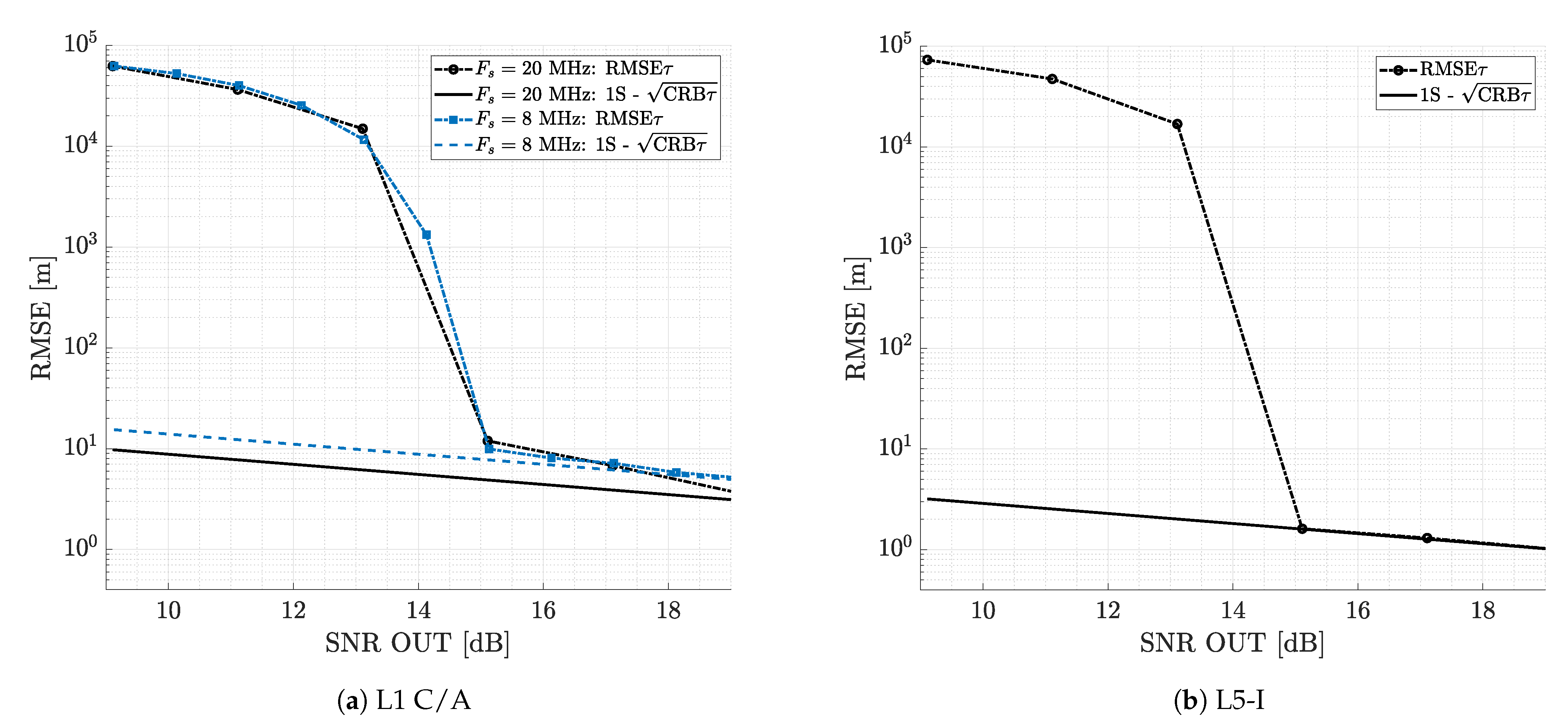
4.1.2. Suboptimal Single Source Estimation

This analysis provides insights into the performance loss when the possible crosstalk is not taken into account. We compare the RMSE results obtained with the 1S-CMLE introduced Section 3.1 with the single source CRB given in Section 2.3. Notice that Δ τ = 1 / 2 L5-I chips = 0.05 L1 C/A chips and Δ τ = 1 L5-I chips = 0.1 L1 C/A chips. The results are shown in Figure 5.
In the sequel, in all the figures presented, the CMLE/CRE behavior can be divided into three distinct regions: (i) in the a priori region, at a low SNR, the estimate behaves as a random variable uniformly distributed on the search area and leads to a very large RMSE; in this case, the estimate is useless for the user; (ii) the threshold region (i.e., where the estimator RMSE drops significantly) is useful to know the minimum SNR at the output of the matched filter to be in optimal operation conditions; and (iii) the asymptotic region is where the estimator behaves correctly, given that the estimator is asymptotically efficient (i.e., convergence to the CRB).
From the GPS L1 C/A results, we can draw three main conclusions: (i) In a dual source context, the single source estimators only converge to the bound for very low values of | Γ | (i.e., 0.01 and 0.1 in the Δ τ = 1 , 1 / 2 , 1 / 4 L1 C/A chips results or only 0.01 in the case of Δ τ = 1 / 8 L1 C/A chips);. In this case, there is no impact of a possible crosstalk. (ii) For higher values of | Γ | , the 1S-CMLE never converges to the 1S-CRB, and therefore, the crosstalk induces a performance degradation. This significantly impacts the receiver performance for | Γ | = 0.5 and for Δ τ = 1 / 8 L1 C/A chips. It is worth pointing out that in such conditions, the estimator RMSE reaches a constant floor, which is typical of a biased estimator (easy to spot in Figure 5d–f). This is due to the fact that for a significant value of | Γ | , the crosstalk distorts the CCF and shifts its maximum. Consequently, even if, for larger | Γ | , the threshold seems to be earlier, the estimated value turns out to be biased. (iii) These results justify the need for dual source estimators or other robust solutions if a possible strong crosstalk is expected. For the GPS L5-I case, we can see the same behavior for Δ τ = 1 L5-I chips and a performance saturation for Δ τ = 1 / 2 L5-I chips (even for | Γ | = 0.1 ). This is because the achievable RMSE with an L5-I signal is far below the corresponding one with the L1 C/A signal (i.e., the L5-I CCF is sharper than the L1 C/A CCF); therefore, small deviations on the CCF have a larger impact on the final performance.

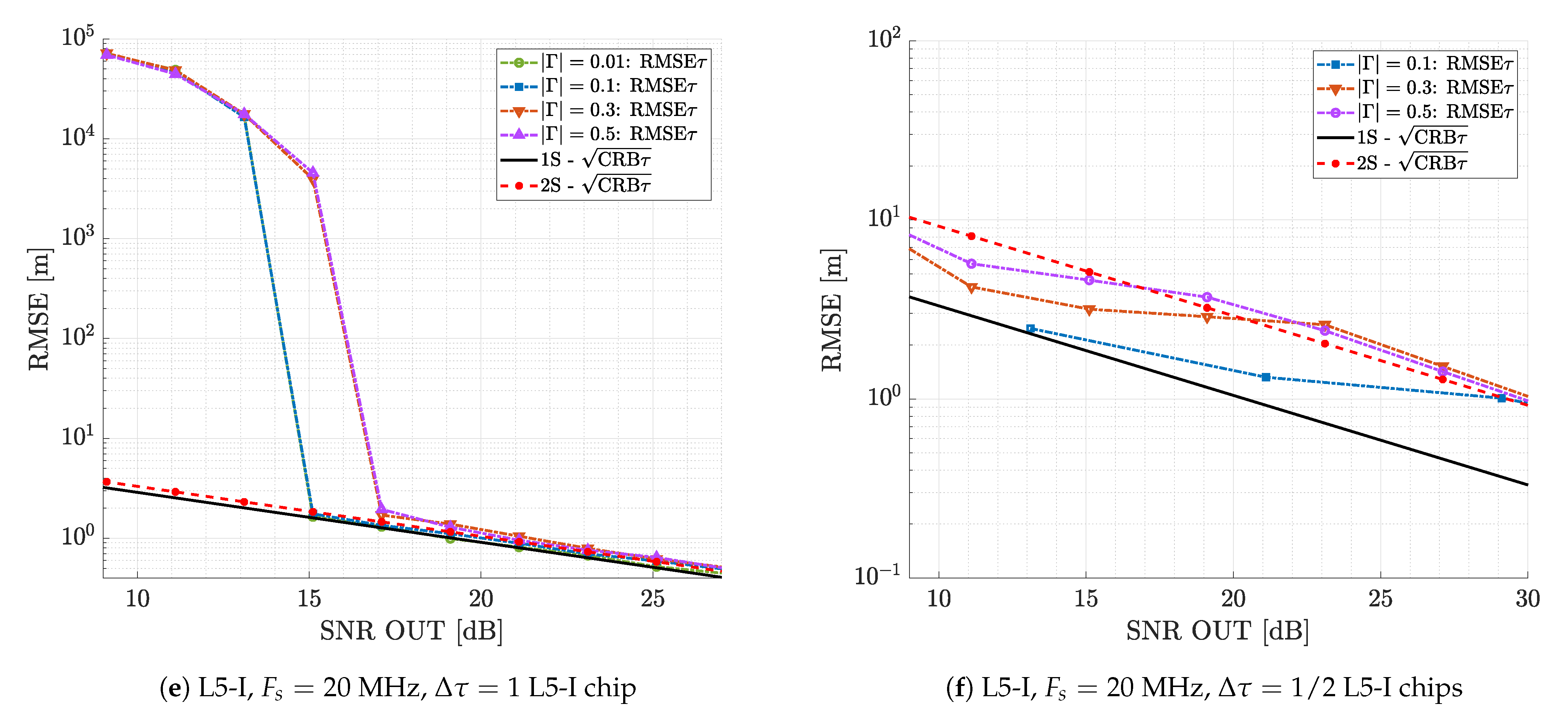
4.2. Optimal Dual Source Estimation

This analysis provides insights into the optimal achievable performance with respect to the single source case. Recall that with respect to the previous case, we know that two sources are present, and the parameters associated with both sources are estimated, either with a CRE or a 2S-CMLE when the CRE does not converge because both sources are too close in time. We compare these dual source estimators with the single and dual source CRBs. Results are shown in Figure 6.
From the results shown in Figure 6, we can draw different conclusions: (i) First, we notice that at a sufficiently high SNR, the estimators converge to the CRB, irrespective of the values of Δ τ and | Γ | , which is a known result for CMLE [48]. This implies that using a dual source estimator and under certain conditions, we can mitigate the impact of any possible crosstalk. (ii) It is also worth pointing out the difference between the 1S-CRB and 2S-CRB, which is limited for most of the range of Δ τ considered in this study. This implies that once the estimator converges to the bound, the crosstalk impact on the estimation performance is limited as well (with respect to the optimal single source case). (iii) The third point is the ability of the CRE to converge to the bound for values as low as Δ τ = 1 / 4 chips ( F s = 8 MHz) for the GPS L1 C/A or 0.1 L1 C/A chips ( F s = 20 MHz) for the GPS L5-I. For the GPS L1 C/A case with Δ τ = 1 / 8 chips or the GPS L5-I case with Δ τ = 0.05 L1 C/A chips, the CRE did not converge, the reason why the results were obtained with the 2S-CMLE. Notice that this threshold can be increased with a better resolution, that is a higher signal bandwidth. (iv) Notice also the strong impact that | Γ | has on the convergence threshold. While for low values such as | Γ | = 0.01 or 0.1 , the convergence is very fast, for larger values, this may imply several dB of difference on the optimal operation point. (v) Lastly, notice that the CMLE performance cannot be below the CRB, as is the case in the plots. This is because of a reduced parameter space search in the implementation, to avoid a huge computational burden.
In any case, we can conclude that (i) for low values of | Γ | and using a dual source estimator, crosstalk has almost no impact, and (ii) for large values of | Γ | , we need a higher SNR in order to mitigate the crosstalk.

4.3. On the Dual Source Estimators’ Robustness: Misspecified Number of Sources

In the previous Section 4.1.2 and Section 4.2, we provided a time-delay estimation performance analysis in a dual source context. First, we considered a single source estimator, in order to assess the impact of a possible crosstalk (i.e., not taken into account) w.r.t. the optimal single source case, and then, we considered dual source estimators to assess the impact w.r.t. the single source case in an optimal setup. A fundamental question of practical interest is: what is the performance of dual source estimators when only one source is present? In other words, what is the robustness of dual source estimators when the number of sources is misspecified? In practice, this is the case of interest, because the crosstalk is not always present.
We assess the performance obtained with a CRE considering two sources, but a single source is present in the signal. For the simulation, we used the same parameters of Doppler frequency and phase as before for the reflected signal, and we simply set the modulus | Γ | to zero. Results for both GPS L1 C/A and GPS L5-I signals are shown in Figure 7, where it is clear that the CRE is robust in the case of a misspecified number of sources. Indeed, it properly estimates the reflected signal parameters and sees the rest as noise. This implies that the CRE is a promising option to mitigate the possible crosstalk.

5. Results and Discussion on Non-Coherent Estimation

Finally, we want to link the variance method to the previous CRBs and maximum likelihood estimation, that is to the corresponding estimation performance, which, to the best of our knowledge, has not been done in the literature. In addition, we also compare the results with a non-coherent CRE (NC-CRE), which must be used in practice to perform long integration times.

5.1. Analysis Setup

Recall that the VE given in (17) is designed to eliminate the contribution of the coherent part of the signal. Therefore, to cover a set of representative case studies, we consider four different scenarios, where for all of them, there are two GPS L1 C/A signals, F s = 8 MHz, Δ τ = 1 / 4 L1 C/A chips, | Γ | = 0.5 , and a total signal duration of 20 ms (i.e., T = 20 ms, T c = 1 ms, and N n c = 20 ; one PRN is 1 ms long). The direct LOS signal is considered to be coherent during the observation time, that is it has the same phase during T. For the reflected signal whose delay we want to estimate in this study and taking into account that we use 20 GPS L1 PRN codes, we consider the following:
  • Scenario #1: 20 PRNs, each one with a different random phase.
  • Scenario #2: four blocks of five PRNs where (i) the first five PRNs have the same phase as the LOS signal and (ii) the other three blocks of five PRNs have three different random phases.
  • Scenario #3: two blocks of 10 PRNs where (i) the first 10 PRNs have the same phase as the LOS signal and (ii) the other two blocks of five PRNs have two different random phases.
  • Scenario #4: four blocks of five PRNs where (i) the first 15 PRNs have the same phase as the LOS signal and (ii) the remaining block of five PRNs has a random phase.
Notice that these four cases cover from the fully non-coherent reflected signal in Scenario #1 to the almost coherent reflected signal in Scenario #4. In these simulations, we arbitrarily set the complex amplitude phase of the reflected path equal to the LOS signal’s one (one could set it to another fixed value without changing the general outputs of this study).

5.2. On the Estimation Performance of the Variance Estimator and Non-Coherent CRE

The RMSE results obtained for the four scenarios with both the VE and NC-CRE are shown in Figure 8. First, notice that the VE performance for a fully non-coherent scenario (#1) reaches the corresponding dual source CRB (i.e., which is almost equivalent to the single source CRB in these scenarios; refer to the middle-left plot of Figure 6) at around 17 dB; then, in this case the estimator is asymptotically efficient and behaves similar to the 1S-CMLE without crosstalk. In contrast, when the coherent part of the reflected signal increases, its performance drastically degrades, and the VE is not a valid approach anymore (i.e., Scenarios #3 and #4), as expected by construction. Therefore, the VE is only useful if considering reflected signals with a dominant non-coherent component such as ocean surfaces, but it is not for specular reflections over ice or for certain land surfaces with a significant coherent signal part. Regarding the NC-CRE, it is asymptotically efficient irrespective of the signal coherency, therefore being a very powerful seamless alternative to the VE. Notice that the NC-CRE for the estimation of the reflected delay does not fully converge to the corresponding 2S-CRB until the convergence of the estimation of the secondary delay (in this case, the LOS delay), at 30 dB, but the performance degradation between the first threshold and 30 dB is minor. Then, both methods have their pros and cons, the VE being easier to implement and the NC-CRE being more robust to the type of surface.

6. Conclusions

In this contribution, we analyzed, from an estimation point of view, the possible crosstalk in ground-based and low altitude airborne GNSS-R. Both the crosstalk impact on standard architectures and possible mitigation strategies were discussed. First, it was found that the single source CMLE performance is not affected by crosstalk if the reflected-to-direct signal amplitude ratio is low enough; otherwise, there is a performance degradation that must be accounted for. Second, it was shown that both CRE and dual source CMLE are asymptotically optimal irrespective of the amplitude ratio, then being a promising crosstalk mitigation strategy. Notice that using the CRE is limited by the time separation among both sources. However, such analysis was performed in a coherent signal context, and in practice, the reflected signal is non-coherently averaged over long integration times. That is the reason why a complementary analysis was provided to assess the performance of an NC-CRE, which was shown to be also asymptotically efficient irrespective of the signal coherency. In contrast, the VE used in the literature was shown to be a valid approach only for non-coherent signals, for which this estimator is asymptotically efficient. Otherwise, for instance in close-to-specular reflections, the VE suffers a significant performance degradation. Then, we can conclude that both the NC-CRE and VE are good ways to mitigate the crosstalk impact, with their pros and cons. Notice that the performance analysis provided in this study investigated the impact of the LOS signal on the reflected one, but the results are also valid to analyze the impact of the reflected signal on the LOS one. The only difference is that the LOS signal is stronger than the reflected signal, or vice versa.
As a side note, the robustness of the CRE for a misspecified number of sources was also discussed. It is also worth pointing out that to avoid the crosstalk, a possible alternative is to exploit large bandwidth Galileo E5 signals, for which a possible parameter estimation performance degradation induced by crosstalk is very unlikely. Finally, another possible way to avoid such crosstalk, not discussed in this contribution, may be to consider antenna arrays with adaptive beamforming capabilities, where a beam can be steered towards the reflection point and a null placed on the direct signal direction of arrival.

Author Contributions

Conceptualization, C.L. and L.O.; formal analysis, C.L. and J.V.-V.; funding acquisition, L.L. and E.C.; methodology, C.L. and L.O.; software, C.L. and L.O.; supervision, J.V.-V. and E.C.; validation, C.L., L.O., J.V.-V., and E.C.; writing—original draft, C.L. and J.V.-V.; writing—review and editing, L.O., L.L., and E.C. All authors read and agreed to the published version of the manuscript.

Funding

This research was partially supported by the CNES and the DGA/AID projects (2019.65.0068. 00.470.75.01, 2018.60.0072.00.470.75.01).

Conflicts of Interest

The authors declare no conflict of interest.

References

  1. Teunissen, P.J.G.; Montenbruck, O. (Eds.) Handbook of Global Navigation Satellite Systems; Springer: Cham, Switzerland, 2017. [Google Scholar]
  2. Zavorotny, V.U.; Gleason, S.; Cardellach, E.; Camps, A. Tutorial on remote sensing using GNSS bistatic radar of opportunity. IEEE Geosci. Remote Sens. Mag. 2014, 2, 8–45. [Google Scholar] [CrossRef] [Green Version]
  3. Jin, S.G.; Cardellach, E.; Xie, F. GNSS Remote Sensing: Theory, Methods and Applications; Springer: Dordrecht, The Netherlands, 2014. [Google Scholar]
  4. Martín-Neira, M. A Passive Reflectometry and Interferometry System (PARIS): Application to Ocean Altimetry. ESA J. 1993, 17, 331–355. [Google Scholar]
  5. Katzberg, S.J.; Garrison, J.L. Utilizing GPS to Determine Ionospheric Delay over the Ocean; NASA Technical Memorandum 4750; 1996. Available online: https://ntrs.nasa.gov/citations/19970005019 (accessed on 11 February 2021).
  6. Anderson, K.D. Determination of Water Level and Tides Using Interferometric Observations of GPS Signals. J. Atmos. Ocean. Technol. 2000, 17, 1118–1127. [Google Scholar] [CrossRef]
  7. Rodriguez-Alvarez, N.; Camps, A.; Vall-llossera, M.; Bosch-Lluis, X.; Monerris, A.; Ramos-Perez, I.; Valencia, E.; Marchan-Hernandez, J.F.; Martinez-Fernandez, J.; Baroncini-Turricchia, G.; et al. Land Geophysical Parameters Retrieval Using the Interference Pattern GNSS-R Technique. IEEE Trans. Geosci. Remote Sens. 2011, 49, 71–84. [Google Scholar] [CrossRef]
  8. Munoz-Martin, J.F.; Perez, A.; Camps, A.; Ribó, S.; Cardellach, E.; Stroeve, J.; Nandan, V.; Itkin, P.; Tonboe, R.; Hendricks, S.; et al. Snow and Ice Thickness Retrievals Using GNSS-R: Preliminary Results of the MOSAiC Experiment. Remote Sens. 2020, 12, 4038. [Google Scholar] [CrossRef]
  9. Roussel, N.; Ramillien, G.; Frappart, F.; Darrozes, J.; Gay, A.; Biancale, R.; Striebig, N.; Hanquiez, V.; Bertin, X.; Allain, D. Sea Level Monitoring and Sea State Estimate Using a Single Geodetic Receiver. Remote Sens. Environ. 2015, 171, 261–277. [Google Scholar] [CrossRef]
  10. Camps, A.; Park, H.; Pablos, M.; Foti, G.; Gommenginger, C.P.; Liu, P.W.; Judge, J. Sensitivity of GNSS-R Spaceborne Observations to Soil Moisture and Vegetation. IEEE J. Sel. Top. Appl. Earth Obs. Remote Sens. 2016, 9, 4730–4742. [Google Scholar] [CrossRef] [Green Version]
  11. Treuhaft, R.N.; Lowe, S.T.; Zuffada, C.; Chao, Y. Two-cm GPS altimetry over Crater Lake. Geophys. Res. Lett. 2001, 28, 4343–4346. [Google Scholar] [CrossRef]
  12. Martín-Neira, M.; Caparrini, M.; Font-Rossello, J.; Lannelongue, S.; Vallmitjana, C.S. The PARIS concept: An experimental demonstration of sea surface altimetry using GPS reflected signals. IEEE Trans. Geosci. Remote Sens. 2001, 39, 142–149. [Google Scholar] [CrossRef] [Green Version]
  13. Martín-Neira, M.; Colmenarejo, P.; Ruffini, G.; Serra, C. Altimetry precision of 1 cm over a pond using the wide-lane carrier phase of GPS reflected signals. Can. J. Remote Sens. 2002, 28, 394–403. [Google Scholar] [CrossRef]
  14. Lowe, S.T.; Zuffada, C.; Chao, Y.; Kroger, P.; Young, L.E.; LaBrecque, J.L. 5-cm precision aircraft ocean altimetry using GPS reflections. Geophys. Res. Lett. 2002, 29, 13-1–13-4. [Google Scholar] [CrossRef] [Green Version]
  15. Lowe, S.T.; Kroger, P.; Franklin, G.; LaBrecque, J.L.; Lerma, J.; Lough, M.; Marcin, M.R.; Muellerschoen, R.J.; Spitzmesser, D.; Young, L.E. A delay/Doppler-mapping receiver system for GPS-reflection remote sensing. IEEE Trans. Geosci. Remote Sens. 2002, 40, 1150–1163. [Google Scholar] [CrossRef]
  16. Rius, A.; Aparicio, J.M.; Cardellach, E.; Martín-Neira, M.; Chapron, B. Sea surface state measured using GPS reflected signals. Geophys. Res. Lett. 2002, 29, 37-1–37-4. [Google Scholar] [CrossRef] [Green Version]
  17. Ruffini, G.; Soulat, F.; Caparrini, M.; Germain, O.; Martín-Neira, M. The eddy experiment: Accurate GNSS-R ocean altimetry from low altitude aircraft. Geophys. Res. Lett. 2004, 31. [Google Scholar] [CrossRef] [Green Version]
  18. Zavorotny, V.U.; Voronovich, A.G. Scattering of GPS Signals from the Ocean with Wind Remote Sensing Application. IEEE Trans. Geosci. Remote Sens. 2000, 38, 951–964. [Google Scholar] [CrossRef] [Green Version]
  19. Marchan-Hernandez, J.F.; Camps, A.; Rodríguez-Álvarez, N.; Valencia, E.; Bosch-Lluis, X.; Ramos-Pérez, I. An efficient algorithm to the simulation of delay—Doppler maps of reflected Global Navigation Satellite System signals. IEEE Trans. Geosci. Remote Sens. 2009, 47, 2733–2740. [Google Scholar] [CrossRef]
  20. Hajj, G.A.; Zuffada, C. Theoretical description of a bistatic system for ocean altimetry using the GPS signal. Radio Sci. 2003, 38. [Google Scholar] [CrossRef]
  21. Rius, A.; Cardellach, E.; Martín-Neira, M. Altimetric analysis of the sea-surface GPS-reflected signals. IEEE Trans. Geosci. Remote Sens. 2010, 48, 2119–2127. [Google Scholar] [CrossRef]
  22. Li, W.; Rius, A.; Fabra, F.; Cardellach, E.; Ribó, S.; Martín-Neira, M. Revisiting the GNSS-R waveform statistics and its impact on altimetric retrievals. IEEE Trans. Geosci. Remote Sens. 2018, 56, 2854–2871. [Google Scholar] [CrossRef]
  23. Park, H.; Pascual, D.; Camps, A.; Martin, F.; Alonso-Arroyo, A.; Carreno-Luengo, H. Analysis of Spaceborne GNSS-R Delay-Doppler Tracking. IEEE J. Sel. Topics Appl. Earth Observ. 2014, 7, 1481–1492. [Google Scholar] [CrossRef]
  24. Martín-Neira, M.; D’Addio, S.; Vitulli, R. Study of Delay Drift in GNSS-R Altimetry. IEEE J. Sel. Topics Appl. Earth Observ. 2014, 7, 1473–1480. [Google Scholar] [CrossRef]
  25. Hu, C.; Benson, C.R.; Rizos, C.; Qiao, L. Impact of Receiver Dynamics on Space-Based GNSS-R Altimetry. IEEE J. Sel. Topics Appl. Earth Observ. 2019, 12, 1974–1980. [Google Scholar] [CrossRef]
  26. Grieco, G.; Stoffelen, A.; Portabella, M. Rationale of GNSS Reflected Delay—Doppler Map (DDM) Distortions Induced by Specular Point Inaccuracies. IEEE J. Sel. Topics Appl. Earth Observ. 2020, 13, 3–13. [Google Scholar] [CrossRef] [Green Version]
  27. Cardellach, E.; Rius, A.; Martín-Neira, M.; Fabra, F.; Nogues-Correig, O.; Ribό, S.; Kainulainen, J.; Camps, A.; D’Addio, S. Consolidating the Precision of Interferometric GNSS-R Ocean Altimetry Using Airborne Experimental Data. IEEE Trans. Geosci. Remote Sens. 2014, 52, 4992–5004. [Google Scholar] [CrossRef]
  28. Martín, F.; Camps, A.; Park, H.; D’Addio, S.; Martín-Neira, M.; Pascual, D. Cross-Correlation Waveform Analysis for Conventional and Interferometric GNSS-R Approaches. IEEE J. Sel. Topics Appl. Earth Observ. 2014, 7, 1560–1572. [Google Scholar] [CrossRef]
  29. Pascual, D.; Camps, A.; Martin, F.; Park, H.; Arroyo, A.A.; Onrubia, R. Precision bounds in GNSS-R ocean altimetry. IEEE J. Select. Topics Appl. Earth Observ. Remote Sens. 2014, 7, 1416–1423. [Google Scholar] [CrossRef]
  30. Martin, F.; D’Addio, S.; Camps, A.; Martín-Neira, M. Modeling and Analysis of GNSS-R Waveforms Sample-to-Sample Correlation. IEEE J. Sel. Topics Appl. Earth Observ. 2014, 7, 1545–1559. [Google Scholar] [CrossRef]
  31. Pascual, D.; Park, H.; Onrubia, R.; Arroyo, A.A.; Querol, J.; Camps, A. Crosstalk Statistics and Impact in Interferometric GNSS-R. IEEE J. Sel. Topics Appl. Earth Observ. 2016, 9, 4621–4630. [Google Scholar] [CrossRef] [Green Version]
  32. Carreno-Luengo, H.; Park, H.; Camps, A.; Fabra, F.; Rius, A. GNSS-R derived centimetric sea topography: An airborne experiment demonstration. IEEE J. Sel. Topics Appl. Earth Observ. 2013, 6, 1468–1478. [Google Scholar] [CrossRef]
  33. Carreno-Luengo, H.; Camps, A.; Ramos-Perez, I.; Rius, A. Experimental Evaluation of GNSS-Reflectometry Altimetric Precision Using the P(Y) and C/A Signals. IEEE J. Sel. Topics Appl. Earth Observ. 2014, 7, 1493–1500. [Google Scholar] [CrossRef]
  34. Li, W.; Cardellach, E.; Fabra, F.; Ribó, S.; Rius, A. Assessment of Spaceborne GNSS-R Ocean Altimetry Performance Using CYGNSS Mission Raw Data. IEEE Trans. Geosci. Remote Sens. 2020, 58, 238–250. [Google Scholar] [CrossRef]
  35. Cardellach, E.; Ao, C.O.; De la Torre, J.M.; Hajj, G.A. Carrier phase delay altimetry with GPS-reflection/occultation interferometry from low earth orbiters. Geophys. Res. Lett. 2004, 31. [Google Scholar] [CrossRef]
  36. Li, W.; Cardellach, E.; Fabra, F.; Rius, A.; Ribó, S.; Martín-Neira, M. First spaceborne phase altimetry over sea ice using TechDemoSat-1 GNSS-R signals. Geophys. Res. Lett. 2017, 44, 8369–8376. [Google Scholar] [CrossRef]
  37. Li, W.; Cardellach, E.; Fabra, F.; Ribo, S.; Rius, A. Lake level and surface topography measured with spaceborne GNSS-reflectometry from CYGNSS Mission: Example for the lake Qinghai. Geophys. Res. Lett. 2018, 45, 13–332. [Google Scholar] [CrossRef]
  38. Lestarquit, L.; Peyrezabes, M.; Darrozes, J.; Motte, E.; Roussel, N.; Wautelet, G.; Frappart, F.; Ramillien, G.; Biancale, R.; Zribi, M. Reflectometry with an Open-Source Software GNSS Receiver: Use Case with Carrier Phase Altimetry. IEEE J. Sel. Topics Appl. Earth Observ. Remote Sens. 2016, 9, 4843–4853. [Google Scholar] [CrossRef]
  39. Cardellach, E.; Li, W.; Rius, A.; Semmling, M.; Wickert, J.; Zus, F.; Ruf, C.S.; Buontempo, C. First Precise Spaceborne Sea Surface Altimetry with GNSS Reflected Signals. IEEE J. Select. Topics Appl. Earth Observ. Remote Sens. 2019, 13, 102–112. [Google Scholar] [CrossRef]
  40. Martin, F.; Camps, A.; Fabra, F.; Rius, A.; Martin-Neira, M.; D’Addio, S.; Alonso, A. Mitigation of Direct Signal Cross-Talk and Study of the Coherent Component in GNSS-R. IEEE Geosci. Remote Sens. Lett. 2015, 12, 279–283. [Google Scholar] [CrossRef]
  41. Das, P.; Ortega, L.; Vilà-Valls, J.; Vincent, F.; Chaumette, E.; Davain, L. Performance Limits of GNSS Code-Based Precise Positioning: GPS, Galileo & Meta-Signals. Sensors 2020, 20, 2196. [Google Scholar]
  42. Ortega, L.; Medina, D.; Vilà-Valls, J.; Vincent, F.; Chaumette, E. Positioning Performance Limits of GNSS Meta-Signals and HO-BOC Signals. Sensors 2020, 20, 3586. [Google Scholar] [CrossRef]
  43. Medina, D.; Ortega, L.; Vilà-Valls, J.; Closas, P.; Vincent, F.; Chaumette, E. Compact CRB for Delay, Doppler and Phase Estimation—Application to GNSS SPP & RTK Performance Characterization. IET Radar Sonar Navig. 2020, 14, 1537–1549. [Google Scholar]
  44. Das, P.; Vilà-Valls, J.; Vincent, F.; Davain, L.; Chaumette, E. A New Compact Delay, Doppler Stretch and Phase Estimation CRB with a Band-Limited Signal for Generic Remote Sensing Applications. Remote Sens. 2020, 12, 2913. [Google Scholar] [CrossRef]
  45. Lubeigt, C.; Ortega, L.; Vilà-Valls, J.; Lestarquit, L.; Chaumette, E. Joint Delay-Doppler Estimation Performance in a Dual Source Context. Remote Sens. 2020, 12, 3894. [Google Scholar] [CrossRef]
  46. Ottersten, B.; Viberg, M.; Stoica, P.; Nehorai, A. Exact and Large Sample Maximum Likelihood Techniques for Parameter Estimation and Detection in Array Processing. In Radar Array Processing; Haykin, S., Litva, J., Shepherd, T.J., Eds.; Springer: Heidelberg, Germany, 1993; Chapter 4; pp. 99–151. [Google Scholar]
  47. Stoica, P.; Nehorai, A. Performances study of conditional and unconditional direction of arrival estimation. IEEE Trans. ASSP 1990, 38, 1783–1795. [Google Scholar] [CrossRef]
  48. Renaux, A.; Forster, P.; Chaumette, E.; Larzabal, P. On the High-SNR Conditional Maximum-Likelihood Estimator Full Statistical Characterization. IEEE Trans. Signal Process. 2006, 54, 4840–4843. [Google Scholar] [CrossRef] [Green Version]
  49. Li, J.; Stoica, P. Efficient mixed-spectrum estimation with applications to target feature extraction. IEEE Trans. Signal Process. 1996, 44, 281–295. [Google Scholar]
  50. Townsend, B.R.; Fenton, P.C.; Van Dierendonck, K.J.; Richard Van Nee, D.J. Performance Evaluation of the Multipath Estimating Delay Lock Loop. Navigation 1995, 42, 502–514. [Google Scholar] [CrossRef]
Figure 1. Typical GNSS-R geometry with the local elevation angle e and the receiver height h.
Remotesensing 13 01085 g001
Figure 2. Geometrical direct to reflected signal time difference Δ τ (ms) for different receiver altitudes. (Right) A zoom in for the small values of receiver height. CCF, cross-correlation function.
Remotesensing 13 01085 g002
Figure 3. (Top) Representative GPS and Galileo signals’ characteristics. ACF peak refers to the first zero-crossing of the ACF. (Bottom) GPS L1 C/A, GPS L5-I, and Galileo E5 ACFs.
Remotesensing 13 01085 g003
Figure 4. Squared modulus of the correlation functions for an L1 C/A signal in the case of crosstalk. In these figures, both signals are in phase ( ϕ 1 = ϕ 0 ), and the amplitude of the LOS crosstalk signal is half of the reflected signal ( | Γ | = 0.5 ).
Remotesensing 13 01085 g004
Figure 5. RMSE for the estimation of the main signal delay τ with 1S-CMLE in the presence of a secondary signal with relative amplitudes | Γ | = 0.01 , 0.1 , 0.3 , 0.5 and different Δ τ and F s , for both GPS L1 C/A and L5-I signals.
Remotesensing 13 01085 g005aRemotesensing 13 01085 g005b
Figure 6. RMSE for the estimation of the main signal delay τ with the relax version of the so-called CLEANestimator algorithm (CRE) (ae) and 2S-CMLE (d,f) in the presence of a secondary signal with relative amplitudes | Γ | = 0.01 , 0.1 , 0.3 , 0.5 and different Δ τ , for both GPS L1 C/A and L5-I signals.
Remotesensing 13 01085 g006aRemotesensing 13 01085 g006b
Figure 7. RMSE for the delay τ estimation considering a GPS L1 C/A signal at F s = 8 MHz in blue and at F s = 20 MHz in black (Left) and a GPS L5-I signal at F s = 20 MHz (right). The case study with a misspecified number of sources: one source is present, but a dual source CRE is used.
Remotesensing 13 01085 g007
Figure 8. RMSE results for the reflected signal delay estimation considering two GPS L1 C/A signals at F s = 8 MHz, Δ τ = 1 / 4 , | Γ | = 0.5 . VE, variance estimator; NC, non-coherent.
Remotesensing 13 01085 g008
Publisher’s Note: MDPI stays neutral with regard to jurisdictional claims in published maps and institutional affiliations.

