Evaluation of Multiple Methods for the Production of Continuous Evapotranspiration Estimates from TIR Remote Sensing

Abstract

Continuous daily estimates of evapotranspiration (ET) spatially distributed at plot scale are required to monitor the water loss and manage crop irrigation needs. Remote sensing approaches in the thermal infrared (TIR) domain are relevant to assess actual ET and soil moisture status but due to lengthy return intervals and cloud cover, data acquisition is not continuous over time. This study aims to assess the performances of 6 commonly used as well as two new reference quantities including rainfall as an index of soil moisture availability to reconstruct seasonal ET from sparse estimates and as a function of the revisit frequency. In a first step, instantaneous in situ eddy-covariance flux tower data collected over multiple ecosystems and climatic areas were used as a proxy for perfect retrievals on satellite overpass dates. In a second step, instantaneous estimations at the time of satellite overpass were produced using the Soil Plant Atmosphere and Remote Sensing Evapotranspiration (SPARSE) energy balance model in order to evaluate the errors concurrent to the use of an energy balance model simulating the instantaneous IRT products from the local surface temperature. Significant variability in the performances from site to site was observed particularly for long revisit frequencies over 8 days, suggesting that the revisit frequency necessary to achieve accurate estimates of ET via temporal upscaling needs to be fewer than 8 days whatever the reference quantity used. For shorter return interval, small differences among the interpolation techniques and reference quantities were found. At the seasonal scale, very simple methods using reference quantities such as the global radiation or clear sky radiation appeared relevant and robust against long revisit frequencies. For infra-seasonal studies targeting stress detection and irrigation management, taking the amount of precipitation into account seemed necessary, especially to avoid the underestimation of ET over cloudy days during a long period without data acquisitions.

1. Introduction

Evapotranspiration (ET) is an important component of the water cycle and its estimation is required to monitor the water loss and manage crop irrigation needs to ensure the efficient use of water in agricultural environments [1]. To reach that goal, spatially distributed and continuous daily estimates of ET at plot scale are needed. These requirements cannot be easily met by existing in situ flux measurements. Remote sensing approaches are then necessary to monitor ET over space and time. Since evapotranspiration is the most efficient way to dissipate energy from the surface, there is a strong coupling between water availability and surface temperature under water stress conditions. Information in the thermal infrared (TIR) domain is commonly used to assess actual evapotranspiration and soil moisture status at relevant space and time scales [2,3]. The revisit intervals of current high spatial resolution TIR missions such as LANDSAT (16 days, 100 m resolution) are insufficient to monitor agricultural water resources management. NASA ECOsystem Spaceborne Thermal Radiometer Experiment on Space Station (ECOSTRESS) was recently deployed to improve temporal sampling of TIR observation (4 days, 40 × 70 m, [4,5]). ESA Copernicus Land Surface Temperature Monitoring (LSTM) has started its preparatory phase and aims to support agricultural water management (3 days, 50 m, [6]). The French Space Agency (CNES) and the Indian Space Research Organization (ISRO) also develop of a new satellite mission called TRISHNA, combining ad hoc features for eco- and especially agro-hydrological applications: a high spatial resolution (50 m) and a high revisit capacity (2 to 3 days) in the thermal infrared domain [7].

Most methods using information in the TIR domain rely on data acquired once-a-day, generally around noon, in late morning or early afternoon. Usually, an instantaneous energy budget is computed at the time of the satellite overpass and provides a single instantaneous latent heat flux estimate (LE), whereas a daily estimation is required for hydrological and agricultural applications, as well as ET sequences over longer periods. Moreover, data availability depends on both the revisit frequency and the presence of cloud cover. To provide temporally continuous ET estimates using remote sensing, instantaneous estimates need to be extrapolated to daily ET with a reconstruction of hourly variations. Moreover, ET dynamic also needs to be reconstructed between two successive available daily ET values, which corresponds to the period between two successive cloud-free images. Interpolation techniques are then commonly used to provide continuous estimates of ET over the season. To do so, ET is usually estimated as the product of a reference quantity to which ET is largely proportional or at least positively correlated (that we call the interpolation reference quantity hereafter) and a scaling factor obtained from the instantaneous ET estimate at the time of the satellite overpass. The scaling factor is usually chosen as the ratio between the instantaneous ET and the instantaneous value of the interpolation reference quantity at the time of the acquisition. The reference quantity must be easy to measure or to estimate every day. The reconstruction of missing ET data between available estimates is then performed by (i) interpolating the scaling factor between remote sensing estimates, (ii) calculating interpolated instantaneous ET from the reference quantity and the interpolated scaling factor, and (iii) extrapolating daily ET each day from the instantaneous value.

The question of extrapolating instantaneous measurements to daily values has received constant attention since thermal infrared remote sensing was proposed to estimate evapotranspiration [8,9]. The main proposed techniques rely on the hypothesis that the scaling factor is preserved during the day [10,11,12]. Components of the radiation budget such as the global radiation R_g [9,13], the extraterrestrial solar radiation R_ext [14,15] have been often used as reference quantities to extrapolate instantaneous measurements to daily ET. The available energy (AE) defined as the difference between the net radiation and the soil heat flux has also been largely used as extrapolation reference quantity and therefore the evaporative fraction (EF), ratio between ET and AE, as the extrapolation reference quantity (e.g., [16,17,18,19,20,21,22]). Reference or potential evapotranspiration have also been used [19,23]. Ref. [24] gave a list of the various scaling factors used in the literature together with the key findings on their performances. However, many studies have underlined that the basic assumption of a preserved scaling factor during the day is not generally met. Ref. [25] underlined that daily self-preservation of the scaling factors is strongly influenced by cloud cover. Sky conditions are then a potential source of error when deriving daily ET [15,23,26]. Refs. [20,27] also showed that the daily course of evaporative fraction is sensitive to soil moisture conditions and vegetation cover and considered the self-preservation as an approximation. Refs. [22,23,24] quantified the divergence between reconstructed daily ET and measured ET, concurrently for various extrapolation reference quantities, showing that most of the reference quantities led to an underestimation of calculated daily ET by 5 to 30% depending on the site and the reference quantity. The lower biases were obtained when using reference quantities directly related to solar radiation.

The interpolation of ET values to fill the gaps between satellite acquisitions has received less attention than the extrapolation to daily values [14,15,19,24,28,29]. Ref. [29] used in situ measurements collected over a variety of land cover types as a proxy for remotely sensed data to evaluate the impact of five interpolation reference quantities and three interpolation techniques. The study focused on daytime mean data to evaluate temporal upscaling at a daily time step. The five interpolation reference quantities ranked among the most commonly used: the incident solar radiation, the available energy, the net radiation, the reference ET described by [30] and the equilibrium evapotranspiration as defined by [31] or [32]. They appeared to be relevant to obtain sequences of daily ET estimates with less than 20% error when considering satellite revisit of 5 days or less. A similar result was obtained by [24]. This precision is sufficient to obtain fairly reliable seasonal ET estimates and to compare inter annual time series. However, [24] showed that it may be too low to monitor rewetting events and water stress for shorter observation periods, as the possibility to capture rapid changes in ET is reduced when satellite revisit period increases. Moreover, most studies regarding ET interpolation assumed perfect retrieval of the flux as no error was introduced into ET data to approximate the uncertainty induced in the estimates of ET from remote sensing data. Since the errors in the remote sensing-based ET estimates propagate into the subsequent reconstruction of the continuous series of daily ET, a degradation of the quality of the retrievals is expected.

A major insight of our study was to deconvolute the respective impacts of remote sensing estimation and interpolation by using, in a first part, in situ data from eddy covariance flux monitoring stations considering no error related to remote sensing estimation, and by using, in a second part, remote sensing estimates of ET which are subject to estimation errors. In situ data were collected over multiple ecosystems and climatic areas. Remote sensing estimations of ET at the time of satellite overpass were obtained using the Soil Plant Atmosphere and Remote Sensing Evapotranspiration (SPARSE) energy balance model ([33,34]). This allowed evaluating the errors concurrent to the use of an energy balance model simulating the instantaneous ET products from the instantaneous surface temperature.

Beyond ET, estimating water stress is important for inferring the surface water status and the root zone soil moisture level [3]. Providing insights into the relative performance of differing temporal upscaling approaches over a large range of various datasets at smaller time scales (i.e., dry-down periods) is crucial (i) to monitor evaporative water loss and determine crop irrigation needs and (ii) to develop the irrigation techniques and management practices necessary to ensure the efficient use of water in agricultural environments. One issue is that under cloudy conditions, the stress is reduced compared to the stress under clear sky conditions, as clouds can sharply reduce evaporative water losses by providing shade or by bringing precipitations. Interpolating ET during a cloudy period without data retrievals between two successive cloud-free days could then lead to underestimate ET over a consequent period and give wrong information about the evaporative water loss. It seems also necessary to have an accurate and easily measurable proxy to highlight actual stress conditions when no instantaneous LE estimates are available because of cloud occurrence. A simple, available, and easily measurable reference quantity that could be introduced into the temporal upscaling to better take the surface water status into account is the precipitation information. Indeed, the amount of rain could be a proxy for the instantaneous water status of the surface and could be used to highlight actual stress conditions. As far as we know, no studies ever used rain information as a reference quantity to reconstruct ET continuous time series.

In this study, the performances of eight different reference quantities were evaluated for different revisit frequencies. They include classical reference quantities already tested on particular sites [29] as well as new ones such as the combination of one classical with a proxy derived from the amount of precipitation in order to constrain the surface water status at the daily time scale. Thus, the objectives of the study are twofold:

• To assess the performances of 8 reference quantities to reconstruct seasonal ET from discontinuous estimates and as a function of the revisit frequency over multiple agricultural ecosystems and climatic areas; an important point within this objective is to test the interest of interpolation reference quantities that introduce information on rain events for resetting the surface water status;
• To estimate the relative importance of the interpolation with respect to the error or uncertainties in the estimates of ET from a remote sensing-based model.

In a first part and as a preamble, we evaluate the reconstruction of daily ET from instantaneous LE estimates on clear sky days in order to quantify the errors induced from the sole extrapolation of instantaneous data to daily ET. In a second part, the reference quantities and the interpolation techniques used in this study are presented and their accuracies are evaluated at seasonal and daily scales. A last section encapsulates a discussion of the results of this study highlighting the efficiency of the temporal interpolation upscaling and giving an overview of the different benefits and disadvantages of the different reference quantities evaluated.

2. Materials and Methods

2.1. Rationale and Outlines of the Method

The reconstruction of continuous evapotranspiration was evaluated over a variety of crop systems including winter, spring and summer arable crops and orchards for two areas in South France, two areas in North Africa, and one area in North Sahel, spanning different water regimes (see Section 2.2). We investigated in detail the different steps affecting the quality of the reconstruction:

Step 1: the estimation of ET at the time of remote sensing measurements, either from in-situ eddy covariance or retrieved at the same locations with the SPARSE energy balance model from surface temperature measurements.

Step 2: interpolation to fill the gaps between days with available instantaneous estimations.

Step 3: extrapolation from instantaneous estimation up to the daily scale.

The aim is to perform a review of the errors concurrent (i) to the chosen reference quantity and method and ii) to the use of the SPARSE energy balance model for simulating the instantaneous evapotranspiration products from the local surface temperatures (see Section 2.3). The impact of the errors in estimating ET was evaluated by comparing the reconstructed time series from the extrapolation and interpolation algorithms to the in situ ET data. In a preliminary step we first evaluated the upscaling of instantaneous observed data under clear sky to the daily scale (so that the extrapolation procedure is evaluated per se). In a second step we evaluated the reconstructed time series of daily ET derived from in situ data (so that the reconstruction procedure combining interpolation and extrapolation is evaluated). In a third step we evaluated the reconstructed time series of daily ET derived from surface temperature at the time of RS measurements (so that the full reconstruction procedure combining interpolation, extrapolation and ET estimation using SPARSE is evaluated). Revisit between 1 and 16 days were tested. Overpass in the morning (10:30), as with Landsat platforms, and sometime after noon (e.g., 13:30), as proposed for possible future missions, were considered. Morning overpass are expected to provide more cloud-free situations (however this may differ from one area and one season to another), while noon overpasses are supposed to provide more adequate information on water stress.

Interpolation between days with available remote sensing data followed simple procedures as proposed by [19,24,29]. ET was estimated as the product of a reference quantity (q), that is easily measured or estimated every day, and a scaling factor (X) obtained from the instantaneous ET estimate at the time of satellite overpass (Figure 1). Usually, X is defined as the ratio between the instantaneous ET (here taken as the instantaneous latent heat flux LE_i) and the instantaneous value of the reference quantity at the time of the acquisition (subscript i):

$${\mathrm{X}}_{\mathrm{i}}=\frac{{\mathrm{LE}}_{\mathrm{i}}}{{\mathrm{q}}_{\mathrm{i}}}$$

(1)

The instantaneous scaling factor X is interpolated between two acquisitions. Thus, for any instant t on a day with no data acquisitions (subscript “interpolated”) with the assumption that X is self-preserved:

$${\mathrm{ET}}_{\mathrm{t}}={\mathrm{q}}_{\mathrm{t}}\times {\mathrm{X}}_{\mathrm{interpolated}}$$

(2)

Several reference quantities were considered including standard reference quantities that were used in previous work related to the amount of incident radiation, the extraterrestrial radiation, the available energy and the potential or the reference ET (see Section 2.4). New reference quantities that were not used in previous studies were introduced in order to account for variation of water status related to precipitation events or evolution of soil moisture in drying events.

Daily estimation of ET is obtained by upscaling the instantaneous estimates (extrapolation). On days with remote sensing data, we used the method developed by [19] which computes the diurnal course of the latent heat flux on the basis of a parametric model of the evaporative fraction with the diurnal courses of solar radiation and relative humidity as inputs [20]: the model is described in Section 2.5. This model accounts for the different behaviors of the evaporative fraction depending on the water status of the surface making it possible to describe non conservative evaporative fraction during the day, in particular in wet conditions. The approach differs from most of the works already presented in the literature which assumed a constant evaporative fraction during the day, leading to a systematic underestimation of the daily evapotranspiration by 10 to 30% that has to be corrected afterwards (e.g., [15,24]).

For days without remote sensing measurements, we had to use another upscaling method since the absence of surface temperature makes it impossible to compute evaporative fraction directly from energy flux estimates. In these situations, the upscaling considered that the ratio between latent heat flux and the reference quantity, in particular for those related to solar radiation, was conservative (which was confirmed for example by the study by [24]).

2.2. In Situ Datasets

Twenty data sets including local meteorological conditions (wind speed, air temperature, humidity, atmospheric pressure, and precipitation), radiation budget (incident and reflected solar radiation, incident and terrestrial longwave radiation and net radiation), surface fluxes (sensible, latent, and soil heat fluxes) collected over 8 different flux tower sites were used to assess the performance of the interpolation methods. They were collected over multiple ecosystems and climatic areas (

Table 1. Main characteristics of the dataset.

Site Name (Country)	Ecosystem	Studied Year	Name Code	Number of Days Studied	ET0 (mm)	Rain (mm)	Maximal Observed LAI (m2 m−2)	Soil Type (%Clay/%Sand)	Irrigation (mm)	Soil Albedo	Energy Balance Closure
Temperate climate
Auradé (FR)	Wheat	2006	Aur W 2006	246	323	369	3.1	32/21	0	0.25	93%
Auradé (FR)	Sunflower	2007	Aur Su 2007	164	394	374	1.7	32/21	0	0.25	88%
Auradé (FR)	Wheat	2008	Aur W 2008	258	307	507	2.4	32/21	0	0.25	89%
Lamasquère (FR)	Wheat	2007	Lam W 2007	269	656	531	4.5	54/12	0	0.25	94%
Lamasquère (FR)	Corn	2008	Lam C 2008	161	416	296	3.8	54/12	50	0.25	83%
Lamasquère (FR)	Wheat	2009	Lam W 2009	237	447	386	1.7	54/12	0	0.25	92%
Lamasquère (FR)	Corn	2010	Lam C 2010	180	452	446	4.1	54/12	130	0.25	79%
Lamasquère (FR)	Corn	2012	Lam C 2012	119	365	342	5.9	54/12	144	0.25	91%
Lamasquère (FR)	Corn	2014	Lam C 2014	126	339	362	5.2	54/12	175	0.25	85%
Lamasquère (FR)	Corn	2015	Lam C 2015	127	384	333	6.6	54/12	140	0.25	98%
Avignon (FR)	Peas	2005	Avi P 2005	160	318	203	2.8	33/14	100	0.25	95%
Avignon (FR)	Wheat	2006	Avi W 2006	246	439	256	5.5	33/14	20	0.25	94%
Avignon (FR)	Sorghum	2007	Avi So 2007	161	501	168	3.0	33/14	80	0.25	95%
Avignon (FR)	Wheat	2008	Avi W 2008	231	415	502	1.9	33/14	20	0.25	95%
Avignon (FR)	Wheat	2012	Avi W 2012	248	460	437	1.1	33/14	0	0.25	96%
Sahelian climate
Wankama-M (NI)	Millet	2009	Wan M 2009	275	867	430	0.4	13/85	0	0.30	91%
Wankama-F (NI)	Savannah	2009	Wan S 2009	262	793	442	0.3	13/85	0	0.30	91%
Semi-arid climate
Kairouan (TU)	Wheat	2012	Kai W 2012	167	381	161	2.1	31/40	0	0.25	60%
Kairouan (TU)	Olive	2012–2015	Kai Or 2012/15	241 365 365 281	141 330 225 223	640 653 626 502	0.2	8/88	0	0.29	55%
Haouz (MO)	Wheat	2004	Hao W 2004	148	338	192	4.1	34/20	170	0.20	93%

). For the detailed description of sites and datasets, see Appendix A. Half-hourly observations of meteorological conditions as well as the components of the energy budget (R_n, H, G, LE) were continuously monitored above the ground or the canopy from complete micro-meteorological eddy-covariance (EC) stations. For sites with an energy balance closure of less than 80%, the closure was forced using the residual method and the corrected LE was computed as R_n − H − G. For other sites, the half-hourly closure was achieved with the conservation of the Bowen ratio H/LE; thus, the corrected LE was computed as (R_n − G)/(1 + H/LE) [35] (Table 1).

2.3. Remote Sensing Estimates of ET—SPARSE Model

The two-source model named Soil Plant Atmosphere and Remote Sensing Evapotranspiration (SPARSE) solves the surface energy balance equations for the soil and the canopy [33]. It was used in the present study for calculating instantaneous evapotranspiration from surface temperature following the methodology described earlier by [34]. Other required inputs were the main meteorological data (solar irradiance R_g, atmospheric irradiance R_a, air temperature T_a, wind speed u_a and air vapor pressure e_a) and information on vegetation height, Leaf Area Index, and fraction cover. The performances of SPARSE for retrieving LE from remotely-sensed surface temperatures were assessed over different datasets including most of the datasets used in the previous study by [34]. Results were satisfactory with RMSE ranging between 40 and 80 W.m⁻², which is in the range of published results [36].

2.4. Reconstruction of Seasonal ET from Instantaneous Latent Heat Flux on Clear Sky Days—Reference Quantities

Temporal upscaling was applied at each site using all combinations of reference quantity and interpolation algorithms. Specifically, it was conducted with data simulating a satellite revisit frequency of 1, 3, 8, and 16 days corresponding to what can be obtained by large field-of-view sensors (MODIS) or well-known high spatial resolution missions (LANDSAT, ASTER) that provide data and estimates of ET from TIR. Three days is in the range of the targeted revisit by projected high spatial resolution TIR missions (TRISHNA, LSTM). In this study, we assume that a day is cloud-free if the observed solar radiation is higher than 85% of the theoretical clear sky radiation; the latter is being computed using a simple radiation model at a specific time corresponding to the choice of the time of the satellite overpass. The theoretical clear sky solar radiation was estimated as the product of the extraterrestrial solar radiation calculated following [37] and a clearness index from [38]. This threshold was selected according to preliminary analyses comparing the model results with observations on known clear-sky days. In order to avoid artifacts or non-representativeness depending on the arbitrarily chosen starting day, all starting days before the first revisit were selected and the resulting output was taken as the average of all configurations.

The height different reference quantities tested are listed in

Table 2. Reference quantities (q) used to reconstruct evapotranspiration (ET).

Symbol Reference Quantities		Main Inputs	Availability
AE	Available Energy	Rn, G	clear sky day at the time of satellite overpass
Rcs	Clear Sky Radiation	Day, time, lat, lon	30 min
Rg	Global Radiation	-	30 min
Rn_FAO	Net Radiation (FAO)	Relative Humidity, Air Temperature, Rg, Rcs, albedo	30 min
LEpot	Potential latent heat flux		30 min
ET0	Reference Evapotranspiration	Relative Humidity, Air Temperature, Rn, G, wind speed	30 min
API	Antecedent Precipitation Index	Day, rain	30 min
Rain	Rain	-	30 min

. For the first six reference quantities, the observed instantaneous ratios (X in Equation (1)) LE_i/AE_i, LE_i/R_gi, LE_i/R_{n_FAO,i}, LE_i/R_cs,i, LE_i/ET_0,i and LE_i/LE_pot,i were respectively interpolated between two dates simulating an acquisition constrained by the absence of clouds (Figure 1). Each of them was then multiplied by their respective reference quantity q and upscaled to reconstruct daily ET on days with no data acquisition (Equation (2)). The daily courses of the different reference quantities were measured (R_g,t) or calculated (R_{n_FAO,t}, R_cs,t, AEt, and LE_pot,t). R_{n_FAO,t} and R_cs,t are calculated according to Appendix B. AEt is computed from Rg as in Equation (9). LE_pot,t is simulated with SPARSE.

Two additional and original approaches that take the rain into account were also developed and tested. The first approach consists in simulating a maximum evaporative fraction (i.e., EF = 1) when a rainfall intensity greater than 2 mm is measured locally. The EF ratio is then interpolated as before between two dates simulating a satellite overpass constrained by the absence of cloud, considering into the series of observed EF the dates for which EF is forced to 1. A threshold value of 2 mm is taken for a rain event, in order to consider only significant wetting (this method is labeled “AE + rain” in what follows). As this assumption may be strong, an alternative approach was also tested: EF is weighted with the Antecedent Precipitation Index of the day (API). The API on day j + 1, in mm, is calculated from that of the previous day j, as follows:

$${\mathrm{API}}_{\mathrm{j}+1}={\mathrm{API}}_{\mathrm{j}}\times 0.85+{\mathrm{rain}}_{\mathrm{j}}$$

(3)

In fact, when a rain greater than 2 mm appears on day j, EF_j+1 is calculated as:

$${\mathrm{EF}}_{\mathrm{j}+1}=\frac{{\mathrm{API}}_{\mathrm{j}+1}}{{\mathrm{API}}_{\max }}$$

(4)

where API_max is the maximum index calculated over the season. The EF ratio is then interpolated between two dates simulating a satellite overpass considering into the series of observed EF the dates for which EF is forced to the ratio between API and API_max (Equation (4); this method is labeled “AE + API” in what follows). This means that the number of observations used for interpolation is increased by the number of rainfall events greater than 2 mm. The decrease in API from Equation (3) is not used to interpolate ET during the dry down, but rather to provide a more realistic estimate of the soil moisture status before each rainfall event, and therefore EF after the rainfall event. As a consequence, an unrealistic increase of EF is probable before the first rainfall of any given period between two successive satellite observations. This effect might be limited when the revisit frequency is large enough, since the occurrence of important dry downs usually coincides with clear sky conditions.

To perform the interpolation of the scaling factor X, we chose a linear technique. Preliminary tests, not described in this article, showed that cubic spline interpolation exhibited periods of very large discrepancies, especially when the revisit frequency was high, consistent with the result of [24,29].

2.5. Reconstruction of Daily ET from Instantaneous Latent Heat Flux

The daily extrapolation approach proposed by [19] was used to build daily ET from an instantaneous estimate of LE derived from instantaneous data over a clear sky day (Figure 2). The approach is based on the reconstruction of the diurnal dynamic of the evaporative fraction. The latter depends on both atmospheric forcing and surface conditions [27]. Ref. [20] introduced an empirical parameterization of the EF diurnal cycle which produces a rather flat EF diurnal cycle under dry conditions but depicts a pronounced concave up shape under wet conditions. Then, for any instant t:

$${\mathrm{EF}}_{\mathrm{t}}=\left[1.2-\left(0.4\times \frac{{\mathrm{R}}_{\mathrm{g},\mathrm{t}}}{{\mathrm{R}}_{\mathrm{g},\max }}+0.5\times \frac{{\mathrm{RH}}_{\mathrm{t}}}{100}\right)\right]\times \frac{{\mathrm{EF}}_{\mathrm{i},\mathrm{obs}}}{{\mathrm{EF}}_{\mathrm{i},\mathrm{sim}}}$$

(5)

$${\mathrm{EF}}_{\mathrm{i},\mathrm{obs}}=\frac{{\mathrm{LE}}_{\mathrm{i}}}{{\mathrm{AE}}_{\mathrm{i}}}$$

(6)

$${\mathrm{AE}}_{\mathrm{i}}={\mathrm{R}}_{\mathrm{n},\mathrm{i}}-{\mathrm{G}}_{\mathrm{i}}$$

(7)

where R_g is the observed global radiation, EF_i,obs is the observed evaporative fraction at the time of the data acquisition, EF_i,sim is the evaporative fraction calculated at the time of the data acquisition using the expression $1.2-\left(0.4\times \frac{{\mathrm{R}}_{\mathrm{g},\mathrm{i}}}{{\mathrm{R}}_{\mathrm{g},\max }}+0.5\times \frac{{\mathrm{RH}}_{\mathrm{i}}}{100}\right)$ and RH is the relative humidity. R_g,max is set to 1000 W.m⁻².

AE_i is the available energy at the time of the data acquisition.

Then:

$${\mathrm{LE}}_{\mathrm{t}}={\mathrm{EF}}_{\mathrm{t}}\times {\mathrm{AE}}_{\mathrm{t}}$$

(8)

With LE_t, the latent heat flux at the instant t and AE_t, the available energy at the same instant reconstructed from:

$${\mathrm{AE}}_{\mathrm{t}}={\mathrm{R}}_{\mathrm{g},\mathrm{t}}\times \frac{{\mathrm{AE}}_{\mathrm{i}}}{{\mathrm{R}}_{\mathrm{g},\mathrm{i}}}$$

(9)

Thus:

$${\mathrm{ET}}_{\mathrm{d}}={{\displaystyle \sum }}^{}{\mathrm{ET}}_{\mathrm{t}}$$

(10)

with ET_t, the evapotranspiration at the instant t (ET_t = LE_t/λ, λ being the latent heat of vaporization) and with ET_d, the daily evapotranspiration. During nighttime, ET_t is set to 0.

LE, R_n and G are available at the time of the satellite overpass. R_g is available at any instant t.

When R_n,i and G_i are not available, thus every day without satellite overpass, the upscaling procedure cannot rely on Equation (4) as in the above method, and ET_d is more simply computed from the sum of ET calculated at each instant t from Equation (2) (${\mathrm{ET}}_{\mathrm{t}}={\mathrm{s}}_{\mathrm{t}}\times {\mathrm{X}}_{\mathrm{interpolated}}$).

2.6. Evaluation of the Results and Statistical Metrics

The algorithms were qualitatively evaluated by comparing the reconstructed ET_d time series and ET_d in situ measurements. The performance scores were quantified using the root mean square error (RMSE), the bias (Bias) and the Nash-Sutcliff Index (NI). In a first part, the performances of the method used to reconstruct daily ET from instantaneous in situ measurements at 13:30 will be evaluated, then the accuracy of the reconstructed ET cumulated over each season will be discussed. In a third part, the reconstruction statistics at the daily time scale separately for cloudy and for clear days will be analyzed.

3. Results

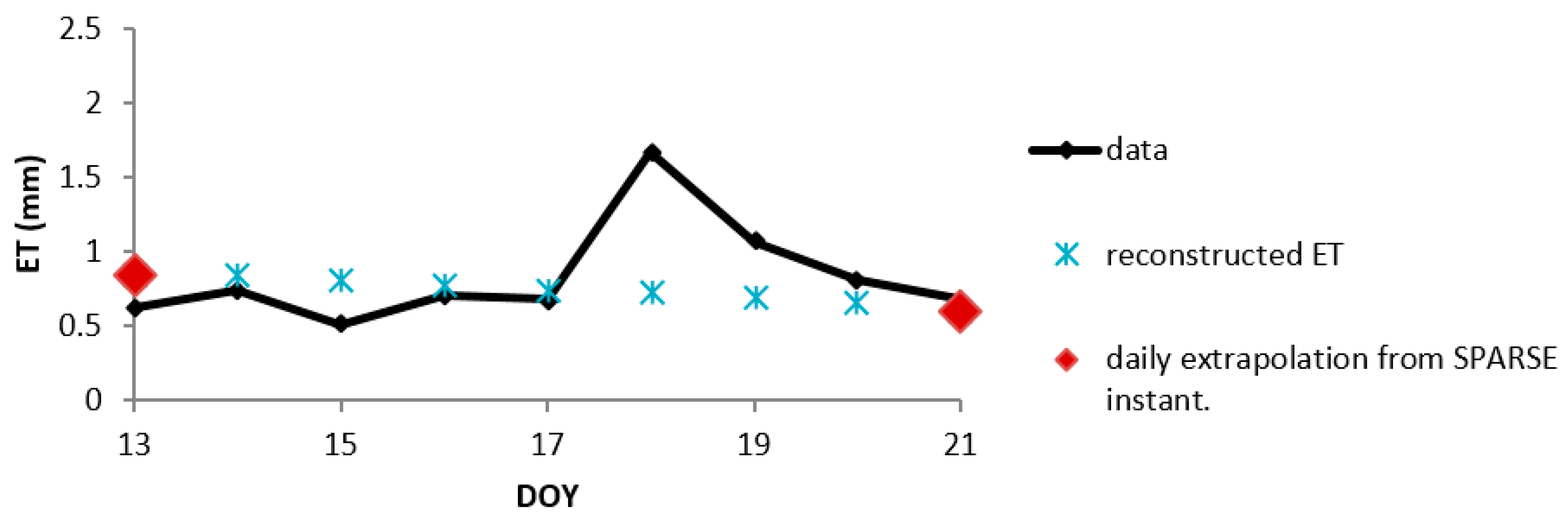
3.1. Reconstruction of Daily ET from Instantaneous Latent Heat Flux on All Clear Sky Days

Performances of the method described in Section 2.5 to reconstruct daily ET from instantaneous in situ measurements at 13:30 are summarized in

Table 3. Statistics of the reconstruction of daily ET from instantaneous in situ latent heat flux and instantaneous remotely-sensed derived latent heat flux on clear sky days at 13:30.

	In Situ Dataset			RS Derived Dataset
	RMSE (mm)	Bias (mm)	NI	RMSE (mm)	Bias (mm)	NI
Aur W 2006	0.94	0.05	0.62	1.14	−0.12	0.48
Aur Su 2007	0.92	0.13	0.26	0.49	0.15	0.79
Aur W 2008	0.76	−0.19	0.49	0.43	−0.29	0.92
Lam W 2007	0.41	0.02	0.83	1.01	−0.67	0.68
Lam C 2008	0.19	0.12	0.71	1.08	−0.45	0.46
Lam W 2009	0.53	0.05	0.79	1.42	−1.08	0.44
Lam C 2010	0.92	0.78	0.72	0.50	−0.23	0.86
Lam C 2012	0.98	0.65	0.33	0.54	0.50	0.71
Lam C 2014	0.88	0.61	0.41	0.64	0.51	0.69
Lam C 2015	0.81	0.25	0.23	0.71	0.35	0.75
Avi P 2005	0.49	0.13	0.92	1.14	−0.46	0.41
Avi W 2006	0.75	0.13	0.79	0.67	0.01	0.83
Avi So 2007	0.74	0.20	0.86	0.52	0.12	0.89
Avi W 2008	0.64	0.26	0.80	0.88	0.33	0.48
Avi W 2012	0.40	0.12	0.88	0.93	−0.35	0.42
Wan M 2009	0.56	0.21	0.70	0.90	−0.18	0.39
Wan S 2009	0.55	0.20	0.82	0.83	0.04	0.30
Kai W 2012	0.64	−0.26	0.38	0.66	0.04	0.60
Kai Or 2012/15	0.60	−0.17	0.75	0.91	−0.07	0.35
Hao W 2004	0.41	0.02	0.83	0.83	0.20	0.54

. Results indicate that, for ground measurements, RMSE vary between 0.19 mm day⁻¹ and 0.98 mm day⁻¹ with 9/20 sites showing RMSE ≤ 0.60 mm day⁻¹ and 6/20 sites showing RMSE > 0.80 mm day⁻¹. These values are within the range of other studies (e.g., [15]) and they confirm the results we obtained in a previous study [19]. For most sites the method showed a small positive bias, lower than 0.20 mm day⁻¹, and a relatively good Nash Index with values greater than 0.70 for 12/20 sites. At 10:30, lower NI were obtained (data not shown). When considering the remote sensing dataset, RMSE ranged between 0.42 and 1.42 mm day⁻¹, which is also in the range of published evaluation of remote sensing estimates of ET (e.x., [36,39]). The use of remote-sensing based instantaneous estimates to reconstruct daily ET increased RMSE for 12/20 sites, in average by 0.45 mm day⁻¹. For most of the other datasets, especially for the summer crops (corn, sorghum, and sunflowers), RMSE improved by 0.28 mm day⁻¹ in average. The results are rather satisfactory: for 10 sites out of 20, NI was beyond 0.6 and for 17 sites, NI was beyond 0.4 (Table 3). On average remote sensing estimates were usually lower than in situ estimates with an average decrease of bias of 0.25 mm day⁻¹.

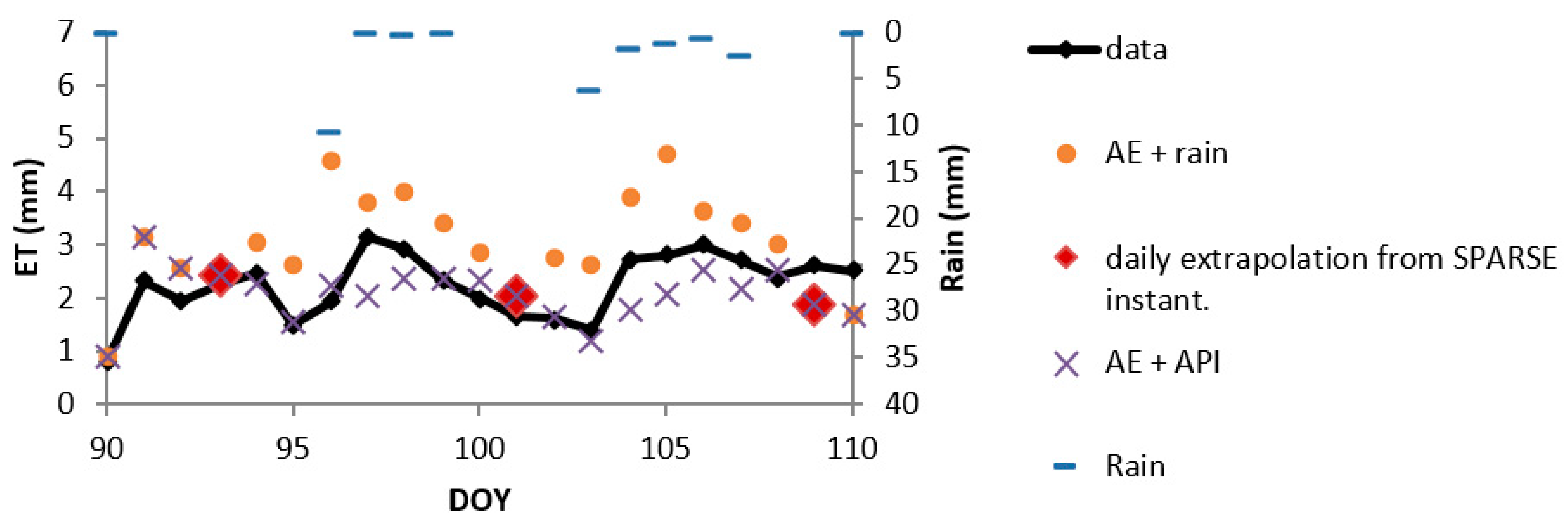
3.2. Accuracy of the Different Reference Quantities at Seasonal Scale

The evaluation of the reconstructed ET cumulated over each season against observed ET is presented in Figure 3 and in

Table A1. Cumulative seasonal evapotranspiration observed (ET_obs, mm) and reconstructed (mm) with the different reference quantitiesand error associated (relative bias in %) for the in situ dataset for a revisit frequency of 1 day. The best reference quantityfor each site is highlighted.

	ETobs	ETAE	ETAE+API	ETAE+rain	ETRcs	ETRg	ETRn_FAO	ETLEpot	ETET0
Aur W 2006	375	344 (−8)	333 (−11)	366 (−2)	401 (+7)	339 (−10)	388 (+4)	498 (+33)	400 (+7)
Aur Su 2007	268	216 (−19)	220 (−18)	274 (+2)	289 (+8)	217 (−19)	273 (+2)	274 (+2)	254 (−5)
Aur W 2008	218	258 (+18)	262 (+20)	297 (+36)	319 (+46)	257 (+18)	242 (+11)	283 (+19)	266 (+22)
Lam W 2007	340	394 (+16)	382 (+12)	440 (+29)	477 (+40)	390 (+15)	389 (+14)	444 (+31)	413 (+22)
Lam C 2008	427	270 (−37)	260 (−39)	309 (−28)	334 (−22)	271 (−37)	270 (−37)	263 (−39)	268 (−37)
Lam W 2009	251	220 (−13)	224 (−11)	285 (+13)	306 (+22)	219 (−13)	270 (+7)	300 (+19)	245 (−3)
Lam C 2010	361	204 (−43)	209 (−42)	260 (−28)	261 (−28)	204 (−43)	204 (−43)	197 (−45)	200 (−45)
Lam C 2012	416	321 (−23)	299 (−28)	357 (−14)	387 (−7)	322 (−23)	303 (−27)	319 (−23)	322 (−23)
Lam C 2014	389	308 (−21)	304 (−22)	352 (−10)	344 (−12)	314 (−19)	312 (−20)	286 (−27)	276 (−29)
Lam C 2015	531	408 (−23)	415 (−22)	390 (−27)	476 (−10)	408 (−23)	408 (−23)	400 (−25)	656 (+24)
Avi P 2005	233	209 (−10)	209 (−10)	209 (−10)	233 (0)	209 (−10)	246 (+6)	266 (+14)	225 (−3)
Avi W 2006	375	337 (−10)	337 (−10)	337 (−10)	393 (+5)	337 (−10)	366 (−3)	424 (+13)	393 (+5)
Avi So 2007	386	338 (−12)	338 (−12)	338 (−12)	372 (−4)	338 (−12)	356 (−8)	352 (−9)	351 (−9)
Avi W 2008	424	351 (−17)	351 (−17)	351 (−17)	427 (+1)	352 (−17)	394 (−7)	482 (+14)	402 (−5)
Avi W 2012	303	278 (−8)	253 (−16)	311 (+3)	326 (+8)	278 (−8)	277 (−8)	309 (+2)	305 (+1)
Wan M 2009	339	257 (−24)	258 (−24)	279 (−18)	278 (−18)	257 (−24)	296 (−13)	265 (−22)	274 (−19)
Wan S 2009	335	262 (−22)	260 (−22)	276 (−18)	285 (−15)	263 (−22)	267 (−20)	264 (−21)	270 (−19)
Kai W 2012	265	280 (+6)	274 (+3)	287 (+9)	308 (+16)	280 (+6)	291 (+10)	279 (+5)	277 (+5)
Kai Or 2012/15	558	510 (−9)	451 (−19)	568 (+2)	524 (−6)	485 (−13)	579 (+4)	551 (−1)	552 (−1)
Hao W 2004	288	279 (−3)	274 (−5)	304 (+6)	318 (+10)	279 (−3)	280 (−3)	284 (−2)	282 (−2)
overall cumul	7082	6044	5913	6590	7058	6019	6411	6740	6631
overall relative bias (%)		−15	−17	−7	−0	−15	−9	−5	−6

and

Table A2. Cumulative seasonal evapotranspiration observed (ETobs, mm) and reconstructed (mm) with the different reference quantitiesand error associated (relative bias in %) for the remotely-sensed derived dataset for a revisit frequency of 1 day. The best reference quantity for each site is highlighted.

	ETobs	ETsparse	ETAE	ETAE+API	ETAE+rain	ETRcs	ETRg	ETRn_FAO	ETLEpot	ETET0
Aur W 2006	375	299	349 (−7)	335 (−11)	365 (−3)	425 (+13)	349 (−7)	362 (−3)	338 (−10)	332 (−11)
Aur Su 2007	268	368	329 (+23)	301 (+12)	343 (+28)	451 (+69)	329 (+23)	335 (+25)	318 (+19)	303 (+13)
Aur W 2008	218	202	261 (+19)	244 (+12)	283 (+29)	382 (+75)	261 (+19)	274 (+26)	241 (+10)	230 (+5)
Lam W 2007	340	533	431 (+27)	409 (+20)	456 (+34)	575 (+69)	431 (+27)	447 (+32)	398 (+17)	393 (+16)
Lam C 2008	427	396	424 (−1)	396 (−7)	435 (+2)	518 (+21)	423 (−1)	434 (+2)	420 (−2)	395 (−8)
Lam W 2009	251	340	370 (+47)	350 (+40)	384 (+53)	393 (+56)	370 (+47)	385 (+53)	353 (+41)	346 (+38)
Lam C 2010	361	401	446 (+24)	430 (+19)	473 (+31)	565 (+57)	447 (+24)	443 (+23)	432 (+20)	425 (+18)
Lam C 2012	416	364	407 (−2)	376 (−10)	432 (+4)	483 (+16)	399 (−4)	385 (−8)	326 (−22)	328 (−22)
Lam C 2014	389	319	367 (−6)	350 (−10)	404 (+4)	400 (+3)	372 (−5)	363 (−7)	342 (−12)	323 (−17)
Lam C 2015	531	371	402 (−24)	388 (−27)	423 (−20)	473 (−11)	402 (−24)	393 (−26)	392 (−26)	384 (−28)
Avi P 2005	233	286	286 (+23)	286 (+23)	286 (+23)	319 (+37)	286 (+23)	293 (+26)	278 (+20)	277 (+19)
Avi W 2006	375	409	429 (+14)	429 (+14)	429 (+14)	481 (+28)	430 (+14)	455 (+21)	413 (+10)	407 (+8)
Avi So 2007	386	404	390 (+1)	390 (+1)	390 (+1)	425 (+10)	391 (+1)	398 (+3)	386 (0)	380 (−1)
Avi W 2008	424	342	368 (−13)	368 (−13)	368 (−13)	440 (+4)	369 (−13)	391 (−8)	344 (−19)	341 (−19)
Avi W 2012	303	357	370 (+22)	343 (+13)	375 (+24)	422 (+39)	370 (+22)	391 (+29)	351 (+16)	349 (+15)
Wan M 2009	339	417	428 (+26)	418 (+23)	434 (+28)	458 (+35)	428 (+26)	438 (+29)	429 (+27)	430 (+27)
Wan S 2009	335	448	285 (−15)	282 (−16)	294 (−12)	304 (−9)	285 (−15)	291 (−13)	288 (−14)	283 (−15)
Kai W 2012	265	297	252 (−5)	239 (−10)	254 (−4)	285 (+7)	252 (−5)	259 (−2)	249 (−6)	243 (−8)
Kai Or 2013	558	484	484 (−13)	448 (−20)	598 (+7)	529 (−5)	484 (−13)	517 (−7)	530 (−5)	482 (−14)
Hao W 2004	288	271	252 (−13)	248 (−14)	273 (−5)	284 (−1)	252 (−13)	255 (−12)	257 (−11)	243 (−16)
overall cumul	7082	7308	7330	7030	7699	8612	7330	7509	7085	6894
overall relative bias vs. measurements (%)	-	3	4	−1	9	22	4	6	0	−3
overall relative bias vs. SPARSE (%)	−3	-	0	−4	5	18	0	3	−3	−6

in Appendix C. Figure 3 presents a summary of the results reference quantity by reference quantity for all sites and the different revisit scenarios. Detailed results for the daily revisit scenario are presented in Table A1 (in-situ dataset) and Table A2 (remote sensing dataset) in Appendix C: cumulated values and error associated for the different reference quantities and the different sites.

When considering the in situ dataset with a daily revisit (Figure 3a and Table A1), overall results showed a consistent tendency to underestimate ET at seasonal scales for all reference quantities with relative biases between 0 and −17%. Relative bias ranged from 0% per season (which correspond to a cumulative difference of 0 mm) to 45% (cumulative difference of 160 mm). Overestimations whatever the reference quantity were obtained only for three datasets (Aur W 2008, Lam W 2007, Kai W 2012, Table A1). Overestimations were observed for 52 cases over 160 (all datasets and all reference quantities considered). Considering only the error induced while evaluating ET cumulated over the entire season, R_cs appeared as the best reference quantity to reconstruct ET for the daily revisit. R_{n_FAO}, ET₀, LE_pot, and AE + rain were also identified as good reference quantities on average, but results were more contrasted from one site to another than with R_cs. In general Rcs provided estimations larger than the other reference quantities.

When considering the interpolation of remote sensing estimates of ET with a daily revisit (Figure 3a and Table A2), the overall results were significantly improved on average for most reference quantities with significant decreases in bias, resulting mostly in slight overestimations (Table A2 in Appendix C). However, when looking at the results of each reference quantity for each seasonal dataset, we noticed a larger scattering of the performances with an increase of high error occurrences (see Figure 3a). Unfortunately, R_cs that was performing the best when considering the in situ dataset provided here a large overestimation and the worse results among all the other reference quantities. The most robust results were obtained with LEpot, but all other reference quantities, except Rcs and at a lesser extent AE + rain, provided acceptable results. It should be noticed that the use of the model to compute instantaneous remotely-sensed fluxes as the base of the ET reconstruction led to overestimate the seasonal ET for most of the sites.

Figure 3b–d present the evaluation of cumulated ET estimated for longer revisits (3, 8 and 16 days). The different reference quantities are fairly robust when the revisit frequency increases to a 3 day return interval, with only a slight degradation of the results compared to the 1 day revisit. From 8 days on, the performances of the interpolation were greatly decreased except for R_cs which allowed the best seasonal ET retrievals for a revisit frequency beyond 8 days. There is a large underestimation for the 16 days revisit frequency, mostly because acquisitions often occur during late stages of dry downs with low ET values and miss many rainfall events (dry down tails are more often sampled at this revisit frequency). This should be corrected by both interpolation methods accounting for rainfall, but only one of them (AE + rain) provide a significant correction. It is probable that for the second method (AE + API) the APImax value is not correctly estimated with such a low revisit and should be decreased to a common “significant rainfall” order of magnitude instead of the maximum API which depends on the maximum rainfall over the season. Large overestimations by the Rcs method are compensated with the overall underestimation at 16 days revisit, therefore leading to a correct estimate at that revisit frequency. Rcs, because it does not account for the decrease in incoming radiation during cloudy periods (i.e., all days with no acquisition when the revisit is daily) tend to overestimate the seasonal ET, resulting in a good bias correction for the in-situ data set.

3.3. Clear Sky vs. Cloudy Days

Since the lack of data between two ET values could result chiefly from either a satellite blank day (clear day but no satellite overpass) or cloud occurrence (satellite overpass but overcast conditions), we analyzed the reconstruction statistics at the daily time scale separately for cloudy and for clear days. Actually, if cloudy days prevent data acquisitions, the revisit frequency of the sensor may also induce clear days without data acquisitions. Seventy-seven percent of the reconstructed chronicles, for an 8-days revisit frequency, showed poorer reconstructions statistics for cloudy days than for clear days where there would be no data because no satellite acquisition. Figure 4 shows the ranking of the reference quantities according to the Nash Index calculated over clear sky days and cloudy days for an everyday and an 8-day revisit frequencies. For example, AE + API was 4 times the best reference quantity (i.e., on 4 datasets), 1 time the second best, etc. to reconstruct ET for cloudy days over a 8-day revisit frequency. For a daily revisit frequency, AE appeared as the best reference quantity to reconstruct ET. For an 8-day revisit frequency, R_cs appeared as the best estimator relatively to others to reconstruct ET for cloudy days, while AE + API is the best reference quantity to reconstruct ET for clear days. Moreover, both were also better than the others except for R_cs to reconstruct ET for cloudy days. Using the information given by the amount of precipitation via API seemed necessary to reconstruct ET.

4. Discussion

4.1. Extrapolation Errors

The self-preservation hypothesis of EF during the day is, according to [22], one of the major sources of bias in extrapolation algorithms. They suggested that improvement in accuracy might also be obtained by a better modelling of available energy. The empirical parameterization of the EF diurnal cycle from [20] used to reconstruct the daily ET from instantaneous measurement on clear sky days (Equation (5)) is consistent with the consensus amongst authors on the observed concave-up shape of most EF diurnal fluctuations. The parameterization originally built for an olive orchard was applied over multiple crops and led to reasonable daily ET estimations for all sites and the large number of climatologic conditions sampled in our datasets (Table 3). Using this shape of EF to reconstruct daily ET appeared as a good method for agricultural applications and performed well as evidenced by a robust bias correction at seasonal timescales compared to a simpler conservative EF assumption [19]. On days with no data acquisitions, the reconstruction of daily ET depends on the reference quantities (Equation (2)). The errors generated from the daily extrapolation of ET on these days with no data are however not significant compared to the errors relevant to the interpolation between available remote sensing estimates itself (not shown).

4.2. Accuracy of the Temporal Upscaling via Interpolation

The use of an interpolation based on the self-preservation of the ratio between LE and the reference quantity are not relevant for long revisit frequency. That result is consistent with the previous studies of [29,40,41]. Interpolated values of the ratio between LE and the reference quantity could then be a source of error and not reflect actual values of ET between image retrievals, especially for long winters without acquisitions or during monsoon periods. The poorer reconstructions statistics for cloudy days than for clear days could explain the tendency to systematically underestimate ET when reconstructing the series. Indeed, when ET is interpolated on a cloudy day, the evaporative demand is reduced, the stress is also lower compared to values predicted with the linear interpolation. The actual ET values are thus more or less strongly underestimated (Figure 5).

There was significant variability in the performances from site to site particularly for long revisit frequencies (over 8 days). Although the specific causes of these differences are not fully understood, this result suggests that the revisit frequency necessary to achieve accurate estimates of ET via temporal upscaling need to be fewer than 8 days whatever the reference quantity used. Dry regions (as Kairouan and Haouz sites) with low ET fluxes seemed to be less affected by the degradation of the revisit frequency than other regions where ET is higher (Table A1 and Table A2), which is quite logical when considering that the variability of ET are lower.

It should be noted that interpolation at the time of satellite acquisition considers sun-synchronous satellite such as Landsat platform, and that it would not be fully adapted to other space systems such as MODIS on Terra and Aqua with variable acquisition time from day to day (see [39]). In these cases, it would be required to interpolate integrated daily value of ET rather than instantaneous values (e.x., [28,29,42]). However, as operations are almost fully linear, this is not supposed to affect significantly our results.

4.3. Choice of the Reference Quantity Depends on the Objectives

The choice of a reference quantity cannot be solved simply: it strongly depends on the objective pursued. At the seasonal scale, for the evaluation of the annual hydrologic budget or inter-annual comparison, we can rely on very simple methods using reference quantities which are available, and which appeared robust against long revisit frequencies, such as R_g or R_cs. While cumulative ET is important for the seasonal water budget, it is also important for agronomical or hydrological applications to look also at the dry down scale, i.e., the day to day variations, during a water stress event for instance. The best reference quantities to reconstruct seasonal ET are not necessarily the ones that perform best when one looks at the dynamics of ET at the event scale. At the event scale, the most efficient reference quantities over all sites are not the same as for the seasonal ET. For infra-seasonal studies aiming at stress detection and irrigation management, accounting for the amount of precipitation at least via API seemed necessary, especially to reduce the underestimation of ET over cloudy days during a long period without data acquisitions.

Figure 6 showed that API is a more relevant index than the method using a threshold value for rain to simulate a maximum EF. However, an overestimation of ET during a dry down period could occur while using API to model EF after a rain event. Actually, two arguments allowed to minimize that possible issue: (i) during cloudy days with no data, the stress is lower and strong dry downs are less likely and (ii) with a high revisit frequency, the risk of missing a dry down is low as the chance of cloud free situation increases. For low revisit frequencies (>8 days), missing dry downs before or after a rain event is a real issue and the use of a surface water balance model providing a better guess of the evolution of water status would be a useful tool to complete the method.

Reference quantities to favor as AE + API are quite complex to implement. Indeed, AE is available only on clear days with acquisitions and involved R_g. Moreover, it seemed valuable to engage a combination of the different reference quantities to minimize underestimation induced on cloudy days for long periods without data.

5. Conclusions

Very strong uncertainties on ET arise from the choice of the reference quantity and only a few studies based on a majority of natural ecosystems (forests and savannahs) have been published on this specific issue of ET interpolation [29]. Our study is based on agricultural ecosystems and the methods developed should be tested and transferred to other ecosystems. This study strongly underlines that the choice of the reference quantity is dependent on the objective: very simple reference quantities such as solar radiation quantities as R_g or R_cs allows relevant reconstructed ET chronicles at the seasonal scale. For stress detection and irrigation management studies, the use of a reference quantity accounting for the amount of precipitation appeared necessary, especially during a long period without data acquisitions.

Other uncertainties are also related to the vector chosen for the production of ET estimations from remote-sensing data (SVAT models or energy balance models in this study). There is little doubt about the possibility of providing a reliable continuous product at low spatial resolution, although the lack of data especially during winter or monsoon periods cause very high uncertainties when rebuilding ET. The question is more complex for the high spatial resolution because of the low availability of thermal information that require looking at more specific interpolation methods which can extend over several weeks.

Today, many datasets from different infra-red sensors are available at different frequencies and spatial resolutions. Some authors have developed another methodological path by proposing interpolation schemes to take advantage of the complementarities between different sensors to combine products from different spatial resolutions. These studies remain few in number and were mainly performed at low resolution [43] and are even rarer at the plot scale ([23,44]).

Few studies have focused on product development at the spatial (plot) and temporal (daily) scales adapted for monitoring the water stress. Actually, a strong decrease in the reconstruction performances appears over 5 to 8 days without ET estimation. Only soil water balance or SVAT model which relies on the spatial distribution of water inputs (irrigation or rain) and soil properties can compensate the lack of TIR data. In the future, producing continuous ET estimations at the plot scale will probably rely not only on remote sensing data acquired at different wavelengths and/or resolutions, but also on their combination with local water balance models constrained at regular intervals by estimates from the TIR domain. Several key directions for further study rely on merging different methods such as the application of data assimilation and fusion techniques in order to producing robust ET estimates to enhance capabilities for monitoring water availability and ecosystem responses.

References

1. Anderson, M.C.; Allen, R.G.; Morse, A.; Kustas, W.P. Use of Landsat thermal imagery in monitoring evapotranspiration and managing water resources. Remote Sens. Environ. 2012, 122, 50–65. [Google Scholar] [CrossRef]
2. Boulet, G.; Olioso, A.; Ceschia, E.; Marloie, O.; Coudert, B.; Rivalland, V.; Chirouze, J.; Chehbouni, G. An empirical expression to relate aerodynamic and surface temperatures for use within single-source energy balance models. Agric. For. Meteorol. 2012, 161, 148–155. [Google Scholar] [CrossRef] [Green Version]
3. Hain, C.R.; Mecikalski, J.R.; Anderson, M.C. Retrieval of an Available Water-Based Soil Moisture Proxy from Thermal Infrared Remote Sensing. Part I: Methodology and Validation. J. Hydrometeorol. 2009, 10, 665–683. [Google Scholar] [CrossRef]
4. Fisher, J.B.; Lee, B.; Purdy, A.J.; Halverson, G.H.; Dohlen, M.B.; Cawse-Nicholson, K.; Wang, A.; Anderson, R.G.; Aragon, B.; Arain, M.A.; et al. ECOSTRESS: NASA’s Next Generation Mission to Measure Evapotranspiration from the International Space Station. Water Resour. Res. 2020, 56, e2019WR026058. [Google Scholar] [CrossRef]
5. Hulley, G.; Shivers, S.; Wetherley, E.; Cudd, R. New ECOSTRESS and MODIS Land Surface Temperature Data Reveal Fine-Scale Heat Vulnerability in Cities: A Case Study for Los Angeles County, California. Remote Sens. 2019, 11, 2136. [Google Scholar] [CrossRef] [Green Version]
6. Koetz, B.; Bastiaanssen, W.; Berger, M.; Defourny, P. High Spatio-Temporal Resolution Land Surface Temperature Mission—A Copernicus candidate mission in support of agricultural monitoring. In IGARSS 2018–2018 IEEE International Geoscience and Remote Sensing Symposium; IEEE: Piscataway, NY, USA, 2018; Available online: https://dial.uclouvain.be/pr/boreal/object/boreal:201985 (accessed on 19 June 2020).
7. Lagouarde, J.; Bhattacharya, B.K.; Crébassol, P.; Gamet, P.; Babu, S.S.; Boulet, G.; Briottet, X.; Buddhiraju, K.M.; Cherchali, S.; Dadou, I.; et al. The Indian-French Trishna Mission: Earth Observation in the Thermal Infrared with High Spatio-Temporal Resolution. In IGARSS 2018–2018 IEEE International Geoscience and Remote Sensing Symposium; IEEE: Piscataway, NY, USA, 2018; pp. 4078–4081. [Google Scholar]
8. Jackson, R.D.; Reginato, R.J.; Idso, S.B. Wheat canopy temperature: A practical tool for evaluating water requirements. Water Resour. Res. 1977, 13, 651–656. [Google Scholar] [CrossRef]
9. Jackson, R.D.; Hatfield, J.L.; Reginato, R.J.; Idso, S.B.; Pinter, P.J. Estimation of daily evapotranspiration from one time-of-day measurements. Agric. Water Manag. 1983, 7, 351–362. [Google Scholar] [CrossRef]
10. Brutsaert, W.; Sugita, M. Application of self-preservation in the diurnal evolution of the surface energy budget to determine daily evaporation. J. Geophys. Res. Atmos. 1992, 97, 18377–18382. [Google Scholar] [CrossRef]
11. Crago, R.D. Conservation and variability of the evaporative fraction during the daytime. J. Hydrol. 1996, 180, 173–194. [Google Scholar] [CrossRef]
12. Nichols, W.E.; Cuenca, R.H. Evaluation of the evaporative fraction for parameterization of the surface energy balance. Water Resour. Res. 1993, 29, 3681–3690. [Google Scholar] [CrossRef]
13. Zhang, L.; Lemeur, R. Evaluation of daily evapotranspiration estimates from instantaneous measurements. Agric. For. Meteorol. 1995, 74, 139–154. [Google Scholar] [CrossRef]
14. Ryu, Y.; Baldocchi, D.D.; Black, T.A.; Detto, M.; Law, B.E.; Leuning, R.; Miyata, A.; Reichstein, M.; Vargas, R.; Ammann, C.; et al. On the temporal upscaling of evapotranspiration from instantaneous remote sensing measurements to 8-day mean daily-sums. Agric. For. Meteorol. 2012, 152, 212–222. [Google Scholar] [CrossRef] [Green Version]
15. Van Niel, T.G.; McVicar, T.R.; Roderick, M.L.; van Dijk, A.I.J.M.; Beringer, J.; Hutley, L.B.; van Gorsel, E. Upscaling latent heat flux for thermal remote sensing studies: Comparison of alternative approaches and correction of bias. J. Hydrol. 2012, 468–469, 35–46. [Google Scholar] [CrossRef]
16. Bastiaanssen, W.; Menenti, M.; Holtslag, A.A.M. A remote sensing surface energy balance algorithm for land (SEBAL). 1. Formulation. J. Hydrol. 1998, 212–213, 198–212. [Google Scholar] [CrossRef]
17. Colaizzi, P.D.; Evett, S.R.; Howell, T.A.; Tolk, J.A. Comparison of Five Models to Scale Daily Evapotranspiration from One-Time-of-Day Measurements. Trans. ASABE 2006, 49, 10. [Google Scholar] [CrossRef]
18. Crago, R.; Brutsaert, W. Daytime evaporation and the self-preservation of the evaporative fraction and the Bowen ratio. J. Hydrol. 1996, 178, 241–255. [Google Scholar] [CrossRef]
19. Delogu, E.; Boulet, G.; Olioso, A.; Coudert, B.; Chirouze, J.; Ceschia, E.; Le Dantec, V.; Marloie, O.; Chehbouni, G.; Lagouarde, J.-P. Reconstruction of temporal variations of evapotranspiration using instantaneous estimates at the time of satellite overpass. Hydrol. Earth Syst. Sci. 2012, 16, 2995–3010. [Google Scholar] [CrossRef] [Green Version]
20. Hoedjes, J.C.B.; Chehbouni, G.; Jacob, F.; Ezzahar, J.; Boulet, G. Deriving daily evapotranspiration from remotely sensed instantaneous evaporative fraction over olive orchard in semi-arid Morocco. J. Hydrol. 2008, 254, 53–64. [Google Scholar] [CrossRef] [Green Version]
21. Suleiman, A.; Crago, R. Hourly and Daytime Evapotranspiration from Grassland Using Radiometric Surface Temperatures. Agron. J. 2004, 96, 384–390. [Google Scholar] [CrossRef]
22. Van Niel, T.G.; McVicar, T.R.; Roderick, M.L.; van Dijk, A.I.J.M.; Renzullo, L.J.; van Gorsel, E. Correcting for systematic error in satellite-derived latent heat flux due to assumptions in temporal scaling: Assessment from flux tower observations. J. Hydrol. 2011, 409, 140–148. [Google Scholar] [CrossRef]
23. Cammalleri, C.; Anderson, M.C.; Gao, F.; Hain, C.R.; Kustas, W.P. Mapping daily evapotranspiration at field scales over rainfed and irrigated agricultural areas using remote sensing data fusion. Agric. For. Meteorol. 2014, 186, 1–11. [Google Scholar] [CrossRef] [Green Version]
24. Guillevic, P.C.; Olioso, A.; Hook, S.J.; Fisher, J.B.; Lagouarde, J.-P.; Vermote, E.F. Impact of the Revisit of Thermal Infrared Remote Sensing Observations on Evapotranspiration Uncertainty—A Sensitivity Study Using AmeriFlux Data. Remote Sens. 2019, 11, 573. [Google Scholar] [CrossRef] [Green Version]
25. Lhomme, J.-P.; Elguero, E. Examination of evaporative fraction diurnal behaviour using a soil-vegetation model coupled with a mixed-layer model. Hydrol. Earth Syst. Sci. 1999, 3, 259–270. [Google Scholar] [CrossRef]
26. Peng, S.; Piao, S.; Wang, T.; Sun, J.; Shen, Z. Temperature sensitivity of soil respiration in different ecosystems in China. Soil Biol. Biochem. 2009, 41, 1008–1014. [Google Scholar] [CrossRef]
27. Gentine, P.; Entekhabi, D.; Chehbouni, A.; Boulet, G.; Duchemin, B. Analysis of evaporative fraction diurnal behaviour. Agric. For. Meteorol. 2007, 143, 13–29. [Google Scholar] [CrossRef] [Green Version]
28. Allen, R.G.; Tasumi, M.; Trezza, R. Satellite-Based Energy Balance for Mapping Evapotranspiration with Internalized Calibration (METRIC)—Model. J. Irrig. Drain. Eng. 2007, 133, 380–394. [Google Scholar] [CrossRef]
29. Alfieri, J.G.; Anderson, M.C.; Kustas, W.P.; Cammalleri, C. Effect of the revisit interval and temporal upscaling methods on the accuracy of remotely sensed evapotranspiration estimates. Hydrol. Earth Syst. Sci. 2017, 21, 83–98. [Google Scholar] [CrossRef] [Green Version]
30. Allen, R.G.; Pereira, L.S.; Raes, D.; Smith, M. Crop evapotranspiration-Guideline for computing crop water requirements. Irrig. Drain. 1998, 56, 300. [Google Scholar]
31. McNaughton, S.J. Serengeti Migratory Wildebeest: Facilitation of Energy Flow by Grazing. Science 1976, 191, 92–94. [Google Scholar] [CrossRef]
32. Raupach, M.R. Combination theory and equilibrium evaporation. Q. J. R. Meteorol. Soc. 2001, 127, 1149–1181. [Google Scholar] [CrossRef]
33. Boulet, G.; Mougenot, B.; Lhomme, J.-P.; Fanise, P.; Lili-Chabaane, Z.; Olioso, A.; Bahir, M.; Rivalland, V.; Jarlan, L.; Merlin, O.; et al. The SPARSE model for the prediction of water stress and evapotranspiration components from thermal infra-red data and its evaluation over irrigated and rainfed wheat. Hydrol. Earth Syst. Sci. Discuss. 2015, 4653–4672. [Google Scholar] [CrossRef] [Green Version]
34. Delogu, E.; Boulet, G.; Olioso, A.; Garrigues, S.; Brut, A.; Tallec, T.; Demarty, J.; Soudani, K.; Lagouarde, J.-P. Evaluation of the SPARSE Dual-Source Model for Predicting Water Stress and Evapotranspiration from Thermal Infrared Data over Multiple Crops and Climates. Remote Sens. 2018, 10, 1806. [Google Scholar] [CrossRef] [Green Version]
35. Twine, T.E.; Kustas, W.P.; Norman, J.M.; Cook, D.R.; Houser, P.R.; Meyers, T.P.; Prueger, J.H.; Starks, P.J.; Wesely, M.L. Correcting eddy-covariance flux underestimates over a grassland. AgFM 2000, 103, 279–300. [Google Scholar] [CrossRef] [Green Version]
36. Kalma, J.D.; McVicar, T.R.; McCabe, M.F. Estimating Land Surface Evaporation: A Review of Methods Using Remotely Sensed Surface Temperature Data. Surv. Geophys. 2008, 29, 421–469. [Google Scholar] [CrossRef]
37. Duffie, J.A.; Beckman, W.A. Solar Engineering of Thermal Processes; John Wiley & Sons: Hoboken, NJ, USA, 2013; ISBN 978-0-470-87366-3. [Google Scholar]
38. Allen, R.G.; Smith, M.; Perrier, A.; Pereira, L.S. An update for the definition of reference evapotranspiration. ICID Bull. 1994, 43, 1–34. [Google Scholar]
39. Allies, A.; Demarty, J.; Olioso, A.; Bouzou Moussa, I.; Issoufou, H.B.-A.; Velluet, C.; Bahir, M.; Maïnassara, I.; Oï, M.; Chazarin, J.-P.; et al. Evapotranspiration Estimation in the Sahel Using a New Ensemble-Contextual Method. Remote Sens. 2020, 12, 380. [Google Scholar] [CrossRef] [Green Version]
40. Farah, H.O.; Bastiaanssen, W.G.M.; Feddes, R.A. Evaluation of the temporal variability of the evaporative fraction in a tropical watershed. Int. J. Appl. Earth Obs. Geoinf. 2004, 5, 129–140. [Google Scholar] [CrossRef]
41. Lu, J.; Tang, R.; Tang, H.; Li, Z.-L. Derivation of Daily Evaporative Fraction Based on Temporal Variations in Surface Temperature, Air Temperature, and Net Radiation. Remote Sens. 2013, 5, 5369–5396. [Google Scholar] [CrossRef] [Green Version]
42. Gallego-Elvira, B.; Olioso, A.; Mira, M.; Castillo, S.R.-; Boulet, G.; Marloie, O.; Garrigues, S.; Courault, D.; Weiss, M.; Chauvelon, P.; et al. EVASPA (EVapotranspiration Assessment from SPAce) Tool: An overview. Procedia Environ. Sci. 2013, 19, 303–310. [Google Scholar] [CrossRef]
43. Bastiaanssen, W.G.M.; Ahmad, M.; Chemin, Y. Satellite surveillance of evaporative depletion across the Indus Basin. Water Resour. Res. 2002, 38, 9-1–9-9. [Google Scholar] [CrossRef]
44. Cammalleri, C.; Anderson, M.C.; Gao, F.; Hain, C.R.; Kustas, W.P. A data fusion approach for mapping daily evapotranspiration at field scale. Water Resour. Res. 2013, 49, 4672–4686. [Google Scholar] [CrossRef]
45. Béziat, P.; Ceschia, E.; Dedieu, G. Carbon balance of a three crop succession over two cropland sites in South West France. Agric. For. Meteorol. 2009, 149, 1628–1645. [Google Scholar] [CrossRef] [Green Version]
46. Garrigues, S.; Olioso, A.; Calvet, J.C.; Martin, E.; Lafont, S.; Moulin, S.; Chanzy, A.; Marloie, O.; Buis, S.; Desfonds, V.; et al. Evaluation of land surface model simulations of evapotranspiration over a 12-year crop succession: Impact of soil hydraulic and vegetation properties. Hydrol. Earth Syst. Sci. 2015, 19, 3109–3131. [Google Scholar] [CrossRef] [Green Version]
47. Chebbi, W.; Boulet, G.; Le Dantec, V.; Lili Chabaane, Z.; Fanise, P.; Mougenot, B.; Ayari, H. Analysis of evapotranspiration components of a rainfed olive orchard during three contrasting years in a semi-arid climate. Agric. For. Meteorol. 2018, 256–257, 159–178. [Google Scholar] [CrossRef]
48. Velluet, C.; Demarty, J.; Cappelaere, B.; Braud, I.; Issoufou, H.B.A.; Boulain, N.; Ramier, D.; Mainassara, I.; Charvet, G.; Boucher, M.; et al. Building a field- and model-based climatology of surface energy and water cycles for dominant land cover types in the cultivated Sahel. Annual budgets and seasonality. Hydrol. Earth Syst. Sci. 2014, 18, 5001–5024. [Google Scholar] [CrossRef] [Green Version]
Figure 1. Illustration of the method to retrieve ET on days with no data acquisitions.
Remotesensing 13 01086 g001
Figure 2. Extrapolation method to reconstruct daily ET from instantaneous measurements the days with data acquisitions.
Remotesensing 13 01086 g002
Figure 3. Relative bias (%) between observed seasonal ET and reconstructed seasonal ET for each reference quantity and (a) 1-day revisit frequency, (b) 3-days revisit frequency, (c) 8-days revisit frequency and (d) 16-days revisit frequency, using in-situ data (red) and remote sensing estimates (blue). Each boxplot presents the statistical results over the different crop cycles.
Remotesensing 13 01086 g003
Figure 4. Number of performance rank occurrences of each reference quantity for cloudy days for 1 day revisit frequency (upper panel), for cloudy days and clear days for an 8-day revisit (middle and bottom panel, respectively).
Remotesensing 13 01086 g004
Figure 5. Reconstructed ET over a cloudy period for an 8 days revisit frequency in Kairouan 2012, with a cloudy sky without precipitations on Day 18.
Remotesensing 13 01086 g005
Figure 6. Reconstructed ET over a rainy period for 8 days revisit frequency in Kairouan 2012.
Remotesensing 13 01086 g006