Abstract
The Gravity Recovery and Climate Experiment (GRACE) mission has measured total water storage change (TWSC) and interpreted drought patterns in an unparalleled way since 2002. Nevertheless, there are few sources that can be used to understand drought patterns prior to the GRACE era. In this study, we extended the gridded GRACE TWSC to 1993 by combining principal component analysis (PCA), least square (LS) fitting, and multiple linear regression (MLR) methods using climate variables as input drivers. We used the extended (climate-driven) TWSC to interpret drought patterns (1993–2019) over the Amazon basin. Results showed that, in the Amazon area with the resolution of 0.5°, GRACE, GRACE follow on, and Swarm had correlation coefficients of 0.95, 0.92, and 0.77 compared with climate-driven TWSCS, respectively. The drought patterns assessed by the climate-driven TWSC were consistent with those interpreted by the Palmer Drought Severity Index and GRACE TWSC. We also found that the 1998 and 2016 drought events in the Amazon, both induced by strong El Niño events, showed similar drought patterns. This study provides a new perspective for interpreting long-term drought patterns prior to the GRACE period.
1. Introduction
As a result of global changes, hydrological extremes such as drought events are increasing. During drought periods, precipitation and soil moisture are dramatically lower than in non-drought periods, while air temperatures are higher than normal with amplitudes varying by land-cover type [1,2]. The length of recovery days presented an evident gradient of increase in mid-latitude regions and of decrease in low-latitude (tropical area) and high-latitude (boreal area) regions; however, recovery was achieved in 60 days in all cases following hydrological drought termination [2]. It is reported that hydrological drought events occurred frequently during the past decade and had a serious influence on the water demand of humankind, agricultural irrigation, and the stability of ecological systems [2,3]. Therefore, it is of great concern in meteorological and hydrological studies to investigate hydrological droughts [4,5,6].
In March 2002, the Gravity Recovery and Climate Experiment (GRACE) mission was jointly launched by the German Aerospace Center (DLR) and National Aeronautical and Spatial Administration (NASA), and it was dedicated to measuring the Earth’s time-variable gravity field [7]. The time-variable gravity field model, observed by the GRACE mission, collects detailed changes in the Earth’s gravity field and infers the total water storage change (TWSC) over large continental regions with unprecedented precision [8]. The GRACE-derived TWSC interprets all information contained in vertical water contents, such as surface water, soil moisture, and ground water, which are clearly of more value to estimate the total water storage during the drought period [9,10]. Thus, the GRACE TWSC holds unique potential to study hydrological drought events over large-scale river basins. It is documented that the GRACE TWSC has made a great contribution to the detection of hydrological droughts [11,12].
The Amazon river basin (ARB) is the largest fringing floodplain of the world’s major river systems. Its drainage area reaches 6.915 million square kilometers, occupying ~40% of the area of South America, almost equivalent to the entire area of Australia. The river volume of the Amazon reaches 219,000 cubic meters per second, which is several times larger than the sum of the other three major rivers, i.e., the Nile River (Africa), the Yangtze River (China), and the Mississippi River (the United States). It is equivalent to the flow of seven Yangtze rivers, accounting for 20% of the world’s river flow, and the discharge of water from the ARB to the ocean contributes to 20–30% of the world’s total water discharge [13,14,15,16]. Furthermore, the Amazon rainforest impacts regional precipitation, runoff, and evapotranspiration, as well as global moisture air mass fluxes [17]. Water evapotranspiration from the ARB accounts for 15% of the world’s total terrestrial evapotranspiration [18]. The ARB not only plays a significant role in the atmospheric and hydrological transport [19] but is also a vital component of the global hydrological cycle and terrestrial ecosystems [20,21,22]. According to the Intergovernmental Panel on Climate Change (IPCC), the incidence and severity of droughts could increase in this basin due to human-induced climate change. Therefore, the assessment of the impacts of extreme droughts in the ARB is of vital importance to develop appropriate drought mitigation strategies [23]. Prior to this, many scholars have monitored water storage changes in the Amazon basin using gravity satellites. Xavier et al. [24] detected changes in water storage in the Amazon basin from 2003 to 2008 using GRACE, hydrological station data, and precipitation data. Chen et al. [25] revealed the temporal and spatial evolution of both nonseasonal and interannual TWSC in the Amazon basin from April 2002 to August 2009 using GRACE monthly gravity solutions. Feng et al. [26] studied the land water reserve change of this basin from 2002 to 2010 using GRACE data. Ning et al. [14] used datasets derived from the products of the Gravity Recovery and Climate Experiment (GRACE), Tropical Rainfall Measuring Mission (TRMM), and the Global Land Data Assimilation System (GLDAS) to assess the extent, intensity, and dynamics of the 2010–2012 abrupt transition from extreme drought to flood in the Amazon. Jin et al. [27] combined GRACE, meteorological, and hydrological data to study the abnormal change in water storage in the Amazon basin from 2010 to 2016. Vergopolan et al. [17] assessed a decade of patterns in evapotranspiration and precipitation over deforested and forest areas using remote sensing (i.e., Moderate-Resolution Imaging Spectroradiometer (MODIS) and TRMM) from 2000 to 2012. Franklin et al. [23] provided a comprehensive characterization of dry spells and extreme drought events in terms of occurrence, persistence, spatial extent, severity, and impacts on streamflow and vegetation in the ARB during the period 1901–2018. Marengo et al. [28] reviews recent progress in the study and understanding of extreme seasonal events in the Amazon region, focusing on droughts and floods. They found that, in the context of the future climate change, drought might intensify through the 21st century.
Several studies have detected extreme hydrological events in the Amazon basin using GRACE; nevertheless, the GRACE mission has only operated since 2002, and there were no similar satellites to estimate the TWSC before 2002. Moreover, there was also an one year blank period (June 2017 to May 2018) between the GRACE and GRACE follow on missions [29]. Most of the past studies only focused on GRACE-dependent applications within the GRACE period (from April 2004 to June 2017). However, it would be beneficial for the drought studies of GRACE to have a longer and uninterrupted time series of total water storage change. The primary objective of this research was to extrapolate the GRACE TWSC fields (0.5° × 0.5°) outside the GRACE period (i.e., 1993–2019) using climate drivers as inputs and study the drought events and their spatial patterns (i.e., distributions) over the Amazon basin prior to the GRACE period.
In this study, we first derived the climate-driven TWSC from 1993 to 2019 by combining three types of methods, that is, principal component analysis (PCA), least square (LS) fitting, and multiple linear regression (MLR). Then, we identified severe drought events that occurred in the Amazon basin using the climate-driven TWSC. We also studied the drought patterns over the Amazon basin during drought periods as identified by the climate-driven TWSC. We show that four severe drought events (i.e., 1996, 1998, 2011, and 2016) occurred in the Amazon basin from 1993 to 2019. Furthermore, the 1998 and 2016 droughts were both induced by strong El Niño events and showed similar drought patterns over the Amazon basin.
2. Materials and Methods
2.1. Materials
2.1.1. Total Water Storage Change Fields
As discussed in Section 1, the first objective of this research was to extend the GRACE-gridded TWSC beyond the GRACE period using climate inputs. In this case, we employed the RL05 monthly mass concentration blocks (mascons) [30] from April 2002 to June 2017, developed by the Center for Space Research (CSR), as the original TWSC data to be extended. The CSR RL05 mascons, with a spatial resolution of 0.5°, are provided in equivalent water depth (cm). These solutions are derived using only GRACE measurements, such that the model is not influenced by external geophysical models or data. Moreover, the time-variable regularization applied in this model ensures that future solutions are not influenced by measurements of past geophysical signals. This means that we no longer have to apply postprocessing to the GRACE spherical harmonic solutions or empirical scaling factors, and we can use these solutions as is for their applications.
The GRACE follow on (GFO) mission has operated since May 2018. The GFO temporal gravity field model, from May 2018 to June 2019, derived by the CSR, were employed to estimate the GFO TWSC over the Amazon basin.
The Swarm mission provides another alternative to infer the temporal gravity field model [31], which can also be used to assess TWSC in the Amazon basin. In this study, the Swarm gravity field models between December 2013 and June 2019, from the Astronomical Institute, Czech Academy of Sciences, with a maximum degree of 40, derived by [27], were used to estimate the Swarm TWSC. To suppress excessive noise at higher orders of the Swarm gravity field models, we only used them completely to a degree and order of 10. The processing strategy was similar to that of GFO, except that we preferred to use 1000 km Gaussian filtering.
2.1.2. Climate Input Data
According to previous studies (e.g., Humprey et al. [32] and Li et al. [33]), the temporal evolution of total water storage is highly related to climate changes such as variations in precipitation and temperature [32,33]. Thus, we could extend the GRACE-gridded TWSC on the basis of its correlations with climate input data. Here, we included the following climate data between January 1992 and September 2019 to extend the CSR mascons: (1) precipitation [25,34,35] from the Climate Prediction Center (CPC); (2) land surface temperature [36] developed by the Global Historical Climatology Network version 2 and the Climate Anomaly Monitoring System (GHCN CAMS); (3) sea surface temperature data [37] provided by the National Oceanic and Atmospheric Administration (NOAA).
2.1.3. In Situ Observations
The total water storage change is mainly driven by variations in ground water, soil moisture, surface water, etc. Although surface water does not represent all total water storage components, it is highly related to the temporal evolution of TWSC, as reported in past studies [25,35]. The time series of monthly water level between 1992 and 2018, measured by 12 in situ gauge stations distributed over the main Amazon tributaries (Figure 1), were used to evaluate the surface water level changes in the Amazon river basin.
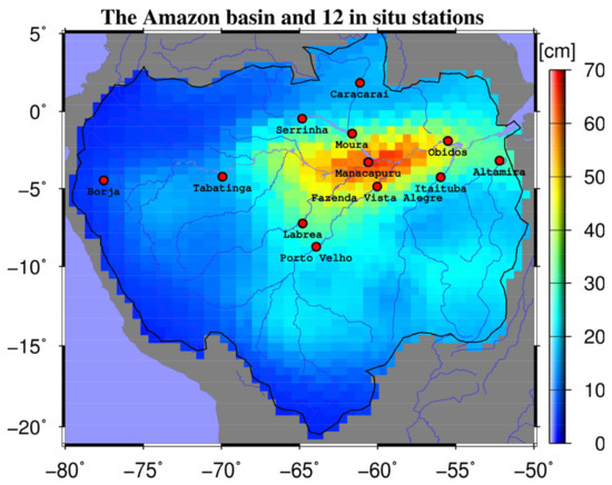
Figure 1.
Location map of 12 in situ gauge stations over the main Amazon tributaries, superimposed by the root mean square (RMS) of Center for Space Research (CSR) mascons.
2.1.4. Palmer Drought Severity Index
In this paper, we employed the monthly Palmer Drought Severity Index (PDSI) over the Amazon basin from June 1992 to December 2014 to verify the reliability of drought patterns estimated by the climate-driven (i.e., extended) total water storage change fields. The PDSI, with a resolution of 2.5°, used in this paper was derived by using the observed surface temperature and precipitation data (Dai [38]).
PDSI is calculated on the basis of a simple two-layer soil water budget model, which takes into account the effects of temperature, precipitation, and underlying surface, in which the effect of temperature is represented by evaporation, and the underlying surface is expressed by available water capacity. The main input parameters of PDSI are precipitation, air temperature, and available water capacity. Table 1 shows the classification of wet and dry grades as a function of the PDSI.

Table 1.
Classification of wet and dry grades.
2.1.5. Data Analysis
More details of the data used in this paper are summarized in Table 2. According to all the above data, the data used in this paper could be roughly divided into four categories: (1) the TWSC from GRACE, Swarm, and GRACE follow on, (2) the climate data including precipitation, land surface temperature, and sea surface temperature, (3) surface water from in situ observation, and (4) the Palmer Drought Severity Index. The GRACE and GRACE follow-on missions are more reliable than Swarm in detecting the TWSC. However, there is a gap of ~1 year between the GRACE and GFO missions, which can be filled by Swarm. Each aspect of the climate data represents the change in a certain factor over the whole process of TWSC. The surface water changes from in situ observation has a high accuracy; however, with just 12 in situ gauge stations, the whole area’s surface water change cannot be adequately represented. The Palmer Drought Severity Index can describe the drought degree of an area (see Table 1); however, as it is just an index, it could not be used to estimate the water deficit during the drought period. Therefore, we used all the above data to comprehensively assess the drought phenomenon in this area.
Table 2.
Data used in this paper.
2.2. Methods
2.2.1. Estimation of the Total Water Storage Changes Using GRACE-FO Gravity Field Models
The specific steps of GFO were as follows: firstly, the C20 term of the GRACE time-variable gravity field models was replaced by the satellite laser ranging (SLR) observation data to improve the accuracy of the second order of the spherical harmonic coefficients [39]. Secondly, the glacial isostatic adjustment (GIA) was removed using the ICE-5G (VM2) model [40]. Thirdly, the north–south strips and high-degree noises [41] in the GFO monthly time-variable gravity field models were removed by de-striping (P5M8) [41] and 300 km Gaussian filtering [42]. Then, the GFO TWSC in the Amazon basin was calculated using the following formula:
where is the average radius of the Earth, is the average density of the Earth, is the density of water, is the longitude of the Earth, is the latitude of the Earth, represents the load Love numbers, is the order of the spherical harmonic coefficient, is the degree of the spherical harmonic coefficient, is the maximum order of the model, is the normalized Legendre function, and and are spherical harmonic coefficients of the residual gravity field, which can be obtained from the following formula:
where and are normalized spherical harmonic coefficients, and are the average values of spherical harmonic coefficients, and is the time in months.
Although some errors of the original model data were eliminated by filtering, the real signal was also weakened. Therefore, the scale method was used to recover the signal attenuation caused by filtering using the following formula:
where is the GLDAS TWSC time variance from the GLDAS model, is the GLDAS TWSC time variance obtained using the spherical harmonic coefficient calculated by GLDAS after different filtering strategies, and is the scale factor of after being calculated from the least square. Thus, the time-varying sequence processed by the same filtering method is multiplied by , resulting in the recovered time variance of TWSC.
2.2.2. Prediction of the Total Water Storage Changes
In this study, the gridded GRACE TWSC over the Amazon basin was extrapolated using three types of methods, i.e., (1) a spatiotemporal decomposition method (principal component analysis, PCA), (2) a time-series separation method (least square, LS), and (3) a machine learning model (multiple linear regression, MLR).
Principal Component Analysis (PCA)
If we forecasted or reconstructed the TWSC at each grid point of a specific region, the calculation would be very large. Therefore, we considered using a spatiotemporal decomposition method (i.e., PCA) to identify the main spatial patterns and the related temporal modes of the GRACE TWSC. PCA allows decomposing the GRACE data into a series of spatial patterns and the related temporal modes [43].
where represents the GRACE data to be decomposed in n-rows and t-columns for each spatial grid and each epoch, respectively. contains n-column spatial patterns, represents n-row temporal modes. The GRACE spatial pattern was assumed to be stable over time [43,44,45]. Moreover, only a few main patterns/modes could interpret almost all the signal variance of the GRACE data; thus, we could extend the GRACE dataset by only extending a few main GRACE temporal modes.
Least Square (LS) Fitting
For deep learning relationships between GRACE data and the potential predictors, the least square (LS) fitting method was employed to decompose the GRACE temporal modes into four components: (1) linear (L), (2) seasonal (S), (3) interannual (I), and (4) residual (R) components [33].
where (i = 1, 2, 3, …, n) represents each main GRACE temporal mode as identified by PCA, and t is the time in epochs. Moreover, the GRACE linear, seasonal, and interannual components were fitted by linear regression, segmented cubic polynomial function, and annual sinewaves, respectively. The residuals were obtained by removing these three components from the GRACE temporal mode. These decomposed components from the GRACE temporal modes are unified as “GRACE components” throughout this paper.
Multiple Linear Regression (MLR)
After decomposing the GRACE temporal modes into four components using Equation (5), we extended all GRACE components, excluding linear trends, using more than three highly correlated climate inputs according to the machine learning method of multiple linear regression (MLR). Here, the GRACE linear trend was usually caused by glacier melts and large human activities; thus, it was hard to predict using climate drivers as inputs. The MLR model allowed extending the GRACE components on the basis of their empirical relationships with the potential input drivers. In this case, the input drivers were the decomposed components from the climate temporal modes. Here, we first estimated the MLR coefficients by training the model using the GRACE components as target variables. Then, we extended the target variables on the basis of the estimated MLR coefficients.
where (i = 1, 2, 3) represents the GRACE seasonal (i = 1), interannual (i = 2), and residual (i = 3) components, respectively, (h = 1, 2, …, n) represents n highly correlated climate inputs, represents the coefficients of MLR which need to be estimated (here, these coefficients were estimated using the least square method) [46], and denotes the error terms. To identify the highly correlated climate inputs for each GRACE component, we firstly decomposed the climate input data (e.g., precipitation and temperature fields) using the same methods as applied to the GRACE data (see Section Principal Component Analysis (PCA) and Section Least Square (LS) Fitting), and then we ranked the components separated from the climate signals (i.e., climate components) on the basis of their correlations as compared with the GRACE component. Lastly, we chose more than three highly correlated climate components as the inputs for extending each GRACE component according to Equation (6).
Signal Compositions
Here, we obtained each extended temporal mode by using the following Equation:
where , , and are the extended components according to Equation (6), and is the decomposed GRACE linear trend.
On account of the stability of GRACE spatial patterns over time [43,45], we could extend the gridded GRACE TWSC as a function of the GRACE spatial patterns (within the GRACE era) and their related temporal modes from the GRACE period (i.e., extended temporal modes). Thus, we obtained the extended TWSC fields/grids as follows:
where represents the extrapolated total water storage change grids (between June 1992 and June 2019 in this study), columns of the matrix are GRACE spatial patterns, rows of are the extended temporal modes, n is the number of spatial grids, and () is the number of selected GRACE patterns/modes (e.g., setting denotes that 100% of the GRACE signals were employed). In this case, we set = 5 because we found that the first five dominant GRACE patterns contributed to almost all (98%) of the GRACE signals over the Amazon basin. The extrapolated TWSC fields were driven by the climate input data as mentioned in Section 2.2.2; thus, we named them “climate-driven TWSC fields” in the context of this paper.
3. Results
3.1. Uncertainty Estimates of the Model Outputs
To test the performance of the models employed in this study, we divided the GRACE period (from April 2002 to June 2017) into two sections, i.e., a training period from April 2002 to March 2012 and a testing period from April 2012 to June 2017. In other words, we used the GRACE TWSC and the climate drivers from April 2002 to March 2012 to train the machine learning model, allowing the machine learning model to derive the climate-driven TWSC for the period of April 2002 to June 2017 using only the climate data as input. The GRACE TWSC between April 2012 and June 2017 was used to test the uncertainties of the climate-driven TWSC in both training and testing periods. As described in Section Multiple Linear Regression (MLR), we predicted each GRACE component and obtained the extended GRACE (climate-driven) TWSC temporal modes by adding together the predicted GRACE seasonal, interannual, and residual components. Appendix A Figure A4 shows the climate-driven TWSC temporal modes in the training and testing periods. Again, these were the sum of the predicted GRACE components, as shown in Appendix A Figure A1, Figure A2 and Figure A3. After obtaining the climate-driven TWSC temporal modes, we finally composed the climate-driven TWSC fields using the leading GRACE spatial patterns (see Appendix A Figure A5) and the climate-driven TWSC temporal modes as described in Section Signal Compositions. Figure 2 shows the correlation coefficients (CCs) and the root-mean-square error (RMSE) of the climate-driven TWSC fields in both training and testing periods, as validated by the GRACE TWSC. The average CCs over the Amazon basin were 0.95 and 0.92 in the training and testing periods, respectively, indicating that our method performed well in both periods. As shown in Figure 2c,d, the RMSE of the climate-driven TWSC fields in the testing period was larger than that in the testing period, which may have been caused by the overfitting problem of the MLR model; that is, the MLR model was overfitted in the training period and, thus, performed worse in the testing period.
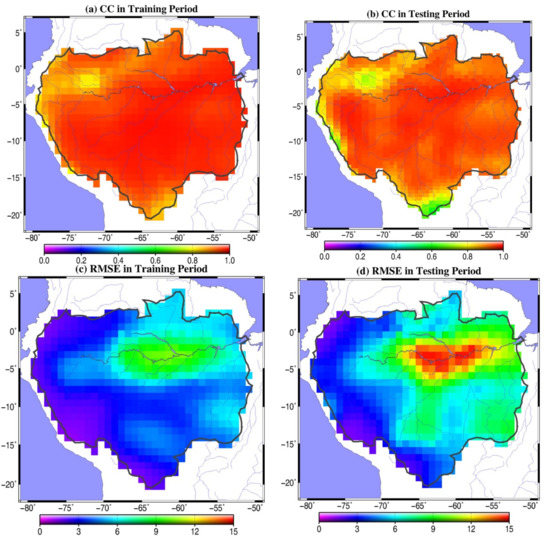
Figure 2.
Correlation coefficients (CCs) of the climate-driven total water storage change (TWSC) fields over the Amazon basin in the (a) training and (b) testing periods compared with the Gravity Recovery and Climate Experiment (GRACE) TWSC. Root-mean-square error (RMSE) of the climate-driven TWSC fields over the Amazon basin in the (c) training and (d) testing periods as evaluated by the GRACE TWSC.
3.2. Climate-Driven Total Water Storage Change Fields
We derived the climate-driven TWSC grids from June 1992 to June 2019 over the Amazon basin using the methods as described in Section 2.2.2. For validation, we calculated the correlations of the climate-driven TWSC as compared to the CSR mascons (R = 0.95), GFO TWSC (R = 0.92), and Swarm TWSC (R = 0.77) at the grid scale (see Figure 3a–c). Figure 3d–f shows the correlations of nonseasonal climate-driven TWSC fields as related to the nonseasonal GRACE, GFO, and Swarm TWSC fields. These TWSC fields at the basin scale were also calculated, as shown in Figure 4a, and we assessed the surface water level in the Amazon basin by averaging the water levels observed at 12 in situ gauge stations (Figure 4b). The correlations (R) of the basin-mean climate-driven TWSC time series as compared to the other TWSCs (i.e., GRACE, GFO, and Swarm) and the surface water level are also shown in Figure 4a. As demonstrated in these pictures, the climate-driven TWSC fields were highly correlated with the CSR mascons, GFO TWSC, and Swarm TWSC at both the grid and the basin scale. Furthermore, the climate-driven TWSC time series were also strongly correlated with the variation in surface water level in the Amazon basin.
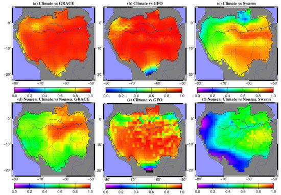
Figure 3.
The correlations of the climate-driven total water storage change fields as compared to the (a) GRACE, (b) GRACE follow-on (GFO), and (c) Swarm TWSC at the grid scale. (d–f) Correlations of the related nonseasonal TWSC fields.
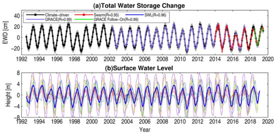
Figure 4.
(a) The climate-driven TWSC time series in the Amazon basin relative to the TWSC from GRACE, GRACE follow-on, and Swarm. (b) The in situ water levels from the 12 in situ gauge stations and the surface water level (blue line) over the Amazon basin. The correlations (R) between the climate-driven TWSC and the other time series are also drawn in the top left of Figure 4a. Note that the surface water level was obtained by averaging all in situ water levels shown in Figure 4b, and the linear trends and mean values of all the time series, for a fair comparison, were removed. The 95% confidence interval for the climate-driven TWSC is drawn in Figure 4a. SWL, surface water level; EWD, equivalent water depth.
3.3. Drought Events Identified from the Basin-Averaged Climate-Driven Total Water Storage Change
Drought events commonly induce strong deficits in the nonseasonal total water storage change [11]. Here, we identified four severe drought events (i.e., 1996, 1998, 2010, and 2016) for the Amazon basin according to the nonseasonal climate-driven TWSC, as shown in Figure 5a. We also, for a comparison, calculated the nonseasonal signals of the GRACE, GFO, Swarm, and SWL time series (see Figure 5a,b), and they all showed large deficits during the four drought periods. Figure 5c shows the basin-averaged PDSI in the Amazon basin, and it also exhibits the minimum values during the identified drought periods, i.e., 1996, 1998, and 2010.
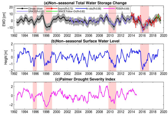
Figure 5.
(a) Nonseasonal signals of the climate-driven, GRACE, GFO, and Swarm TWSC, (b) nonseasonal surface water level, and (c) basin-averaged Palmer Drought Severity Index (PDSI) in the Amazon basin. The red areas represent drought periods identified from the climate-driven TWSC time series. The 95% confidence interval for the nonseasonal climate-driven TWSC is drawn in Figure 5a. EWD, equivalent water depth.
3.4. Drought Patterns Interpreted from the Climate-Driven Total Water Storage Change Fields
Drought/flood patterns can be interpreted from TWSC anomalies [25]. In order to study the drought patterns over the Amazon basin, we derived the yearly climate-driven TWSC anomalies at each grid point (0.5° resolution), as shown in Figure 6. Here, the yearly climate-driven TWSC anomalies were obtained by averaging the nonseasonal TWSC from July of the previous year to June of the current year (e.g., the 1993 climate-driven TWSC anomalies are the mean during July 1992 through June 1993). For verification, we used the same strategy to derive the yearly PDSI and yearly GRACE TWSC anomalies over the Amazon basin (see Figure 7 and Figure 8). The yearly climate-driven TWSC anomalies allowed interpreting that the drought pattern in 1998 was similar to that in 2016, i.e., the droughts mainly occurred in the northeast of the Amazon basin (as shown in Figure 6). These may have been linked to two significant El Niño events (i.e., in 1997/1998 and 2015/2016) reported by Juan et al. (2016). In 1996 and 2011, as interpreted from the yearly climate-driven TWSC anomalies, the central and southwestern regions of the Amazon basin suffered more severe drought events than the northeastern regions (Figure 6). Compared to the climate-driven TWSC anomalies (Figure 6), the yearly GRACE TWSC anomalies showed very close spatial patterns during the drought periods of 2011/2016, and the yearly PDSI exhibited similar drought patterns in 1996/1998 (see Figure 7 and Figure 8), thus verifying the reliability of the drought patterns interpreted from our climate-driven TWSC. Table 3 lists the basin-averaged values of climate-driven TWSC, GRACE TWSC, and PDSI over the Amazon basin. The results suggest that the drought events which occurred in 1998 and 2016 were more severe than those which occurred in 1996 and 2016.
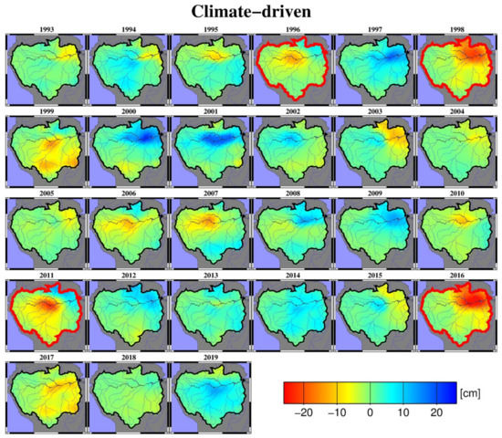
Figure 6.
Yearly drought patterns as interpreted from the climate-driven TWSC. Note that the yearly drought patterns are the mean nonseasonal TWSC from July of the previous year to June of the current year (e.g., the 1993 drought patterns are the mean during July 1992 through June 1993).
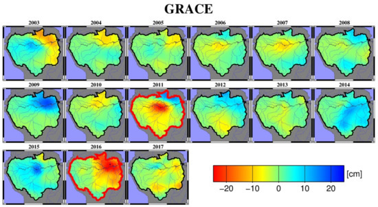
Figure 7.
Yearly drought patterns as interpreted from the GRACE TWSC. Note that the yearly drought patterns are the mean nonseasonal TWSC from July of the previous year to June of the current year (e.g., the 1993 drought patterns are the mean during July 1992 through June 1993).
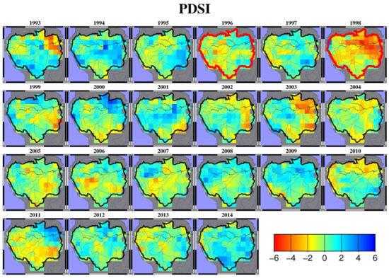
Figure 8.
Yearly drought patterns as interpreted from the Palmer Drought Severity Index (PDSI). Note that the yearly drought patterns are the mean nonseasonal TWSC or PDSI from July of the previous year to June of the current year (e.g., the 1993 drought patterns are the mean during July 1992 through June 1993).
Table 3.
Average climate-driven TWSC, GRACE TWSC, and PDSI over the Amazon basin in the four drought years (i.e., 1996, 1998, 2011, and 2016).
4. Discussions
To estimate the performance of the combination method, we used GRACE data from April 2002 to March 2012 to train the machine learning model (i.e., MLR) and then predicted the climate-driven TWSC for the period of April 2012 to June 2017. The GRACE data from April 2012 to June 2017 were employed to test the uncertainties of the climate-driven TWSC. We found that the climate-driven TWSC fit well with the GRACE data in both training and testing periods (see Figure 2), indicating that our combined method performed well in deriving the climate-driven TWSC for the Amazon basin. We used the GRACE data from April 2002 to June 2017 as the target variable to train the predictive model (i.e., MLR) and to derive the climate-driven TWSC for the period between 1992 and 2019 using climate data (i.e., precipitation, land temperature, and sea surface temperature) as input drivers. We employed GRACE-FO from June 2018 to June 2019 and Swarm TWSC from December 2013 to June 2019 to validate the climate-driven TWSC. The climate-driven (i.e., extended) TWSC grids fit well to the GRACE, GRACE follow on, and Swarm TWSC fields at both the grid and the basin scale (see Figure 3 and Figure 4); furthermore, they were also highly correlated with the evolution of surface water level evaluated at 12 in situ gauge stations in the Amazon basin (see Figure 4b). These results confirmed the reliability of the climate-driven TWSC derived in this study. According to previous studies (e.g., Li et al. [33]), the nonseasonal signal of the TWSC can be used to detect drought events. In this case, we removed the seasonal signal of the climate-driven TWSC and used the nonseasonal climate-driven TWSC time series to detect the drought events which occurred in the Amazon basin between 1992 and 2019. Four severe drought events (i.e., 1996, 1998, 2011, and 2016) were identified using the nonseasonal signal of climate-driven TWSC. During the drought periods, the nonseasonal signals of GRACE TWSC, Swarm TWSC, surface water level, and PDSI in the Amazon also exhibited significant anomalies (i.e., large negative values). We derived the drought patterns from 1993 to 2019 using the climate-driven TWSC fields over the Amazon basin and focused analysis on the four severe drought periods. We found that the 1998 and 2016 droughts, both related to strong El Niño events that occurred in 1997/1998 and 2015/2016, had almost the same drought pattern, while the 1996 and 2011 droughts showed different spatial patterns as compared to 1998/2016. These different patterns in the south and north of the basin could be related to the impact of intense deforestation in the south, potentially leading to reduced infiltration at this location and increased runoff to the floodplain [17]. The drought patterns interpreted from climate-driven TWSC are reliable as validated by the GRACE TWSC and PDSI fields.
5. Conclusions
In this study, we detected the drought events that were occurred in the Amazon basin using the climate driven TWSC (1993–2019) as derived by combining PCA, LS, and MLR methods.
Firstly, we used the GRACE TWSC and the climate drivers from April 2002 to March 2012 to train the machine learning model, which allows the machine learning model for deriving the climate-driven TWSC for the period April 2002 to June 2017 using only the climate data as input. The GRACE TWSC was used to test the uncertainties of the climate-driven TWSC in both training and testing periods. The results show that the average correlation coefficients of the climate driven TWSC as compared to the GRACE TWSC over the Amazon basin were 0.95 and 0.92 in the training and testing periods, respectively, indicating that our method per-formed well.
The climate-driven TWSC grids from June 1992 to June 2019 over the Amazon basin were derived based on the combined method. We found that the climate-driven TWSC fields were highly correlated with the CSR mascons, GFO TWSC, and Swarm TWSC at both grid and basin scales. Furthermore, the basin-averaged climate-driven TWSC time series was strongly correlated with the variation of surface water level in the Amazon basin.
We identified four severe drought events (i.e., 1996, 1998, 2010, and 2016) for the Amazon basin according to the nonseasonal climate-driven TWSC, which coincides with the results as detected by GRACE, GFO, Swarm, SWL, and PDSI. We also found that the drought pattern in 1998 was similar to that in 2016, i.e., droughts were mainly occurred in the northeast of the Amazon basin.
This study provides a new perspective for understanding TWSC-induced drought patterns prior to the GRACE period or during the gap between the GRACE and GRACE-FO missions.
Author Contributions
K.T. conceived the original idea, performed the study, designed the methodology, and wrote the paper. Z.W. contributed to the interpretation of the results. F.L. developed the codes and drawn the figures. C.L., Y.X., and Y.G. revised the paper. All authors have read and agreed to the published version of the manuscript.
Funding
This study is supported by the NSFC (China), under Grants 41274032, 41474018, 41429401, 41774019, and 41704011, 41974007.
Data Availability Statement
CSR MASCON: http://www2.csr.utexas.edu/grace/RL05_mascons.html (accessed on 15 March 2021); GRACE Follow-On: http://isdcftp.gfz-potsdam.de/grace-fo/Level-2/CSR/RL06/ (accessed on 15 March 2021); Swarm data: http://icgem.gfz-potsdam.de/series (accessed on 15 March 2021); Precipitation: https://www.esrl.noaa.gov/psd/data/gridded/tables/precipitation.html (accessed on 15 March 2021); Land surface temperature: https://www.esrl.noaa.gov/psd/data/gridded/tables/temperature.html (accessed on 15 March 2021); Sea surface; temperature: https://www.esrl.noaa.gov/psd/data/gridded/tables/sst.html (accessed on 15 March 2021); Climate indices: https://www.esrl.noaa.gov/psd/data/climateindices/list/ (accessed on 15 March 2021); In situ observations: www.ore-hybam.org; PDSI: https://climatedataguide.ucar.edu/climate-data/palmer-drought-severity-index-pdsi (accessed on 15 March 2021).
Acknowledgments
The authors thank the following data providers CSR, GFZ, NOAA, CPC, SO HYBAM, and NCAR-RDA for making the data available: GRACE mascon; GRACE follow on data; Swarm data; climate data; In situ water levels; and PDSI.
Conflicts of Interest
The authors declare no conflict of interest.
Appendix A

Figure A1.
Seasonal components of the five leading GRACE temporal modes (black lines) relative to the model outputs in the training (red lines) and testing periods (green lines).
Figure A1.
Seasonal components of the five leading GRACE temporal modes (black lines) relative to the model outputs in the training (red lines) and testing periods (green lines).


Figure A2.
Interannual components of the five leading GRACE temporal modes (black lines) relative to the model outputs in the training (red lines) and testing periods (green lines).
Figure A2.
Interannual components of the five leading GRACE temporal modes (black lines) relative to the model outputs in the training (red lines) and testing periods (green lines).


Figure A3.
Residual components of the five leading GRACE temporal modes (black lines) relative to the model outputs in the training (red lines) and testing periods (green lines).
Figure A3.
Residual components of the five leading GRACE temporal modes (black lines) relative to the model outputs in the training (red lines) and testing periods (green lines).


Figure A4.
Five leading GRACE temporal modes (black lines) relative to the composed ones in the training (red lines) and testing periods (green lines).
Figure A4.
Five leading GRACE temporal modes (black lines) relative to the composed ones in the training (red lines) and testing periods (green lines).


Figure A5.
Five leading GRACE spatial patterns as identified using PCA.
Figure A5.
Five leading GRACE spatial patterns as identified using PCA.

References
- Ahmadi, B.; Ahmadalipour, A.; Moradkhani, H. Hydrological drought persistence and recovery over the CONUS: A mul-ti-stage framework considering water quantity and quality. Water Res. 2019, 150, 97–110. [Google Scholar] [CrossRef]
- Yu, Z.; Wang, J.; Liu, S.; Rentch, J.S.; Sun, P.; Lu, C. Global gross primary productivity and water use efficiency changes under drought stress. Environ. Res. Lett. 2017, 12, 014016. [Google Scholar] [CrossRef]
- Zhang, D.; Liu, X.; Bai, P. Assessment of hydrological drought and its recovery time for eight T tributaries of the Yangtze River (China) based on downscaled GRACE data. J. Hydrol. 2019, 568, 592–603. [Google Scholar] [CrossRef]
- Zalewski, M.; McClain, M.; Eslamian, S. New challenges and dimensions of Ecohydrology—Enhancement of catchments sustainability potential. Ecohydrol. Hydrobiol. 2016, 16, 1–3. [Google Scholar] [CrossRef]
- Jassey, V.E.J.; Reczuga, M.K.; Zielińska, M.; Sowińska, S.; Robroek, B.J.M.; Mariotte, P.; Seppey, C.; Lara, E.; Barabach, J.; Słowiński, M.; et al. Tipping point effect in plant-fungal interactions under severe drought causes abrupt rise in peatland ecosystem respiration. Global Change Biol. 2017, 24, 972–986. [Google Scholar] [CrossRef]
- Peng, B.; Xiaomang, L.; Yongqiang, Z.; Changming, L. Incorporating vegetation dynamics noticeably improved performance of hydrological model under vegetation greening. Sci. Total Environ. 2018, 643, 610–622. [Google Scholar]
- Tapley, B.D.; Bettadpur, S.; Watkins, M.; Reigber, C. The gravity recovery and climate experiment: Mission overview and early results. Geophys. Res. Lett. 2004, 31, 09607. [Google Scholar] [CrossRef]
- Swenson, S.C.; Wahr, J.M. Methods for inferring regional surface-mass anomalies from Gravity Recovery and Climate Experiment (GRACE) measurements of time-variable gravity. J. Geophys. Res. Space Phys. 2002, 107, ETG3. [Google Scholar] [CrossRef]
- Andersen, O.B.; Seneviratne, S.I.; Hinderer, J.; Viterbo, P. GRACE-derived terrestrial water storage depletion associated with the 2003 European heat wave. Geophys. Res. Lett. 2005, 32. [Google Scholar] [CrossRef]
- Frappart, F.; Ramillien, G. Monitoring Groundwater Storage Changes Using the Gravity Recovery and Climate Experiment (GRACE) Satellite Mission: A Review. Remote Sens. 2018, 10, 829. [Google Scholar] [CrossRef]
- Thomas, A.C.; Reager, J.T.; Famiglietti, J.S.; Rodell, M. A GRACE-based water storage deficit approach for hydrological drought characterization. Geophys. Res. Lett. 2014, 41, 1537–1545. [Google Scholar] [CrossRef]
- Chao, N.; Wang, Z.; Jiang, W.; Chao, D. A quantitative approach for hydrological drought characterization in southwestern China using GRACE. Hydrogeol. J. 2016, 24, 893–903. [Google Scholar] [CrossRef]
- Hall, A.C.; Schumann, G.J.-P.; Bamber, J.L.; Bates, P.D. Tracking water level changes of the Amazon Basin with space-borne remote sensing and integration with large scale hydrodynamic modelling: A review. Phys. Chem. Earth 2011, 36, 223–231. [Google Scholar] [CrossRef]
- Ning, N.; Wanchang, Z.; Huadong, G.; Natarajan, I. 2010–2012 drought and flood events in the amazon basin inferred by grace satellite observations. J. Appl. Remote Sens. 2015, 9, 096023. [Google Scholar]
- Clark, E.A.; Sheffield, J.; Van Vliet, M.T.H.; Nijssen, B.; Lettenmaier, D.P. Continental Runoff into the Oceans (1950–2008). J. Hydrometeorol. 2015, 16, 1502–1520. [Google Scholar] [CrossRef]
- Nepstad, D.C.; Stickler, C.M.; Filho, B.S.; Merry, F. Interactions among Amazon land use, forests and climate: Prospects for a near-term forest tipping point. Philos. Trans. R. Soc. B Biol. Sci. 2008, 363, 1737–1746. [Google Scholar] [CrossRef]
- Vergopolan, N.; Fisher, J.B. The impact of deforestation on the hydrological cycle in Amazonia as observed from remote sensing. Int. J. Remote Sens. 2016, 37, 5412–5430. [Google Scholar] [CrossRef]
- Field, C.B.; Behrenfeld, M.J.; Randerson, J.T.; Falkowski, P. Primary Production of the Biosphere: Integrating Ter- restrial and Oceanic Components. Science 1998, 281, 237–240. [Google Scholar] [CrossRef]
- Malhi, Y.; Roberts, J.T.; Betts, R.A.; Killeen, T.J.; Li, W.; Nobre, C.A. Climate Change, Deforestation, and the Fate of the Amazon. Science 2008, 319, 169–172. [Google Scholar] [CrossRef]
- Cox, P.M.; Betts, R.A.; Collins, M.; Harris, P.P.; Huntingford, C.; Jones, C.D. Amazonian forest dieback under climate-carbon cycle projections for the 21st century. Theor. Appl. Clim. 2004, 78, 137–156. [Google Scholar] [CrossRef]
- Nobre, C.A.; Sellers, P.J.; Shukla, J. Amazonian Deforestation and Regional Climate Change. J. Clim. 1991, 4, 957–988. [Google Scholar] [CrossRef]
- Suyog, C.; Yadu, P.; Emilio, M.; Gonzalo, M. Multi-decadal hydrologic change and variability in the Amazon River basin: Understanding terrestrial water storage variations and drought characteristics. Hydrol. Earth Syst. Sci. 2019, 23, 2841–2862. [Google Scholar]
- Paredes-Trejo, F.; Barbosa, H.A.; Giovannettone, J.; Kumar, T.V.L.; Thakur, M.K.; Buriti, C.D.O. Long-Term Spatiotemporal Variation of Droughts in the Amazon River Basin. Water 2021, 13, 351. [Google Scholar] [CrossRef]
- Xavier, L.; Becker, M.; Cazenave, A.; Longuevergne, L.; Llovel, W.; Filho, O.C.R. Interannual variability in water storage over 2003–2008 in the Amazon Basin from GRACE space gravimetry, in situ river level and precipitation data. Remote Sens. Environ. 2010, 114, 1629–1637. [Google Scholar] [CrossRef]
- Chen, J.L.; Wilson, C.R.; Tapley, B.D. The 2009 exceptional Amazon flood and interannual terrestrial water storage change observed by GRACE. Water Resour. Res. 2010, 46. [Google Scholar] [CrossRef]
- Feng, W.; Lemoine, J.M.; Zhong, M.; Xu, H. Monitoring Land Water Change in The Amazon Basin from 2002 to 2010 Using GRACE. Chin. J. Geophys. 2012, 55, 814–821. [Google Scholar]
- Jin, Z.; Jin, T. Combined GRACE and Meteorological and Hydrological Data to Study the Relationship between the Abnormal Change of Water Storage and Extreme Climate ENSO in The Amazon from 2010 to 2016. Geod. Geodyn. 2019, 39, 199–203. [Google Scholar]
- A Marengo, J.; Espinoza, J.C. Extreme seasonal droughts and floods in Amazonia: Causes, trends and impacts. Int. J. Clim. 2016, 36, 1033–1050. [Google Scholar] [CrossRef]
- Da Encarnação, J.T.; Visser, P.; Arnold, D.; Bezdek, A.; Doornbos, E.; Ellmer, M.; Guo, J.; Ijssel, J.V.D.; Iorfida, E.; Jäggi, A.; et al. Description of the multi-approach gravity field models from Swarm GPS data. Earth Syst. Sci. Data 2020, 12, 1385–1417. [Google Scholar] [CrossRef]
- Save, H.; Bettadpur, S.; Tapley, B.D. High-resolution CSR GRACE RL05 mascons. J. Geophys. Res. Solid Earth 2016, 121, 7547–7569. [Google Scholar] [CrossRef]
- Lück, C.; Kusche, J.; Rietbroek, R.; Löcher, A. Time-variable gravity fields and ocean mass change from 37 months of kinematic Swarm orbits. Solid Earth 2018, 9, 323–339. [Google Scholar] [CrossRef]
- Humphrey, V.; Gudmundsson, L.; Seneviratne, S.I. A global reconstruction of climate-driven subdecadal water storage variability. Geophys. Res. Lett. 2017, 44, 2300–2309. [Google Scholar] [CrossRef]
- Li, F.; Kusche, J.; Rietbroek, R.; Wang, Z.; Forootan, E.; Schulze, K.; Lück, C. Comparison of Data-Driven Techniques to Reconstruct (1992–2002) and Predict (2017–2018) GRACE-Like Gridded Total Water Storage Changes Using Climate Inputs. Water Resour. Res. 2020, 56, 026551. [Google Scholar] [CrossRef]
- Chen, M.; Shi, W.; Xie, P.; Silva, V.B.S.; Kousky, V.E.; Higgins, R.W.; Janowiak, J.E. Assessing objective techniques for gauge-based analyses of global daily precipitation. J. Geophys. Res. Space Phys. 2008, 113, 113. [Google Scholar] [CrossRef]
- Chen, J.L.; Wilson, C.R.; Tapley, B.D.; Yang, Z.L.; Niu, G.Y. 2005 drought event in the Amazon River basin as measured by GRACE and estimated by climate models. J. Geophys. Res. Space Phys. 2009, 114, 05404. [Google Scholar] [CrossRef]
- Fan, Y.; Dool, H.V.D. Climate prediction center global monthly soil moisture data set at 0.5° resolution for 1948 to present. J. Geophys. Res. 2004, 109, D10102. [Google Scholar] [CrossRef]
- Reynolds, R.W.; Rayner, N.A.; Smith, T.M.; Stokes, D.C.; Wang, W. An improved in situ and satellite SST analysis for climate. J. Clim. 2002, 15, 1609–1625. [Google Scholar] [CrossRef]
- Dai, A. Characteristics and trends in various forms of the Palmer Drought Severity Index during 1900. J. Geophys. Res. Space Phys. 2011, 116. [Google Scholar] [CrossRef]
- Cheng, M.; Ries, J.C.; Tapley, B.D. Variations of the Earth’s figure axis from satellite laser ranging and GRACE. J. Geophys. Res. Solid Earth 2011, 116. [Google Scholar] [CrossRef]
- Peltier, W. Global Glacial Isostasy and the Surface of the Ice-Age Earth: The ICE-5G (VM2) Model and GRACE. Annu. Rev. Earth Planet. Sci. 2004, 32, 111–149. [Google Scholar] [CrossRef]
- Swenson, S.C.; Wahr, J.M.; Milly, P.C.D. Estimated accuracies of regional water storage variations inferred from the Gravity Recovery and Climate Experiment (GRACE). Water Resour. Res. 2003, 39, 375–384. [Google Scholar] [CrossRef]
- Wahr, J.; Molenaar, M.; Bryan, F. Time variability of the earth’s gravity field: Hydrological and oceanic effects and their possible detection using grace. J. Geophys. Res. Solid Earth 1998, 103, 30205–30230. [Google Scholar] [CrossRef]
- Forootan, E.; Kusche, J.; Loth, I.; Schuh, W.-D.; Eicker, A.; Awange, J.; Longuevergne, L.; Diekkrueger, B.; Schmidt, M.; Shum, C.K. Multivariate prediction of total water storage anomalies over West Africa from multi-satellite data. Surv. Geophys. 2014, 35, 913–940. [Google Scholar] [CrossRef]
- Church, J.A.; White, N.J.; Coleman, R.; Lambeck, K.; Mitrovica, J.X. Estimates of the regional distribution of sea level rise over the 1950–2000 period. J. Clim. 2004, 17, 2609–2625. [Google Scholar] [CrossRef]
- Becker, M.; Meyssignac, B.; Xavier, L.; Cazenave, A.; Alkama, R.; Decharme, B. Past terrestrial water storage (1980–2008) in the Amazon Basin reconstructed from GRACE and in situ river gauging data. Hydrol. Earth Syst. Sci. 2011, 15, 533–546. [Google Scholar] [CrossRef]
- Haario, H.; Laine, M.; Mira, A.; Saksman, E. DRAM: Efficient adaptive MCMC. Stat. Comput. 2006, 16, 339–354. [Google Scholar] [CrossRef]


Publisher’s Note: MDPI stays neutral with regard to jurisdictional claims in published maps and institutional affiliations. |
© 2021 by the authors. Licensee MDPI, Basel, Switzerland. This article is an open access article distributed under the terms and conditions of the Creative Commons Attribution (CC BY) license (http://creativecommons.org/licenses/by/4.0/).