Abstract
Generally, there is an inconsistency between the total regional crop area that was obtained from remote sensing technology and the official statistical data on crop areas. When performing scale conversion and data aggregation of remote sensing-based crop mapping results from different administrative scales, it is difficult to obtain accurate crop planting area that match crop area statistics well at the corresponding administrative level. This problem affects the application of remote sensing-based crop mapping results. In order to solve the above problem, taking Fucheng County of Hebei Province in the Huanghuaihai Plain of China as the study area, based on the Sentinel-2 normalized difference vegetation index (NDVI) time series data covering the whole winter wheat growth period, the statistical data of the regional winter wheat planting area were regarded as reference for the winter wheat planting area extracted by remote sensing, and a new method for winter wheat mapping that is based on similarity measurement indicators and their threshold optimizations (WWM-SMITO) was proposed with the support of the shuffled complex evolution-University of Arizona (SCE-UA) global optimization algorithm. The accuracy of the regional winter wheat mapping results was verified, and accuracy comparisons with different similarity indicators were carried out. The results showed that the total area accuracy of the winter wheat area extraction by the proposed method reached over 99.99%, which achieved a consistency that was between the regional remote sensing-based winter wheat planting area and the statistical data on the winter wheat planting area. The crop recognition accuracy also reached a high level, which showed that the proposed method was effective and feasible. Moreover, in the accuracy comparison of crop mapping results based on six different similarity indicators, the winter wheat distribution that was extracted by root mean square error (RMSE) had the best recognition accuracy, and the overall accuracy and kappa coefficient were 94.5% and 0.8894, respectively. The overall accuracies of winter wheat that were extracted by similarity indicators, such as Euclidean distance (ED), Manhattan distance (MD), spectral angle mapping (SAM), and spectral correlation coefficient (SCC) were 94.1%, 93.9%, 93.3%, and 92.8%, respectively, and the kappa coefficients were 0.8815, 0.8776, 0.8657, and 0.8558, respectively. The accuracy of the winter wheat results extracted by the similarity indicator of dynamic time warping (DTW) was relatively low. The results of this paper could provide guidance and serve as a reference for the selection of similarity indicators in crop distribution extraction and for obtaining large-scale, long-term, and high-precision remote sensing-based information on a regional crop spatial distribution that is highly consistent with statistical crop area data.
1. Introduction
In recent years, with the gradual expansion of research on climate change and food security, statistical data on crop planting areas have become irreplaceable [1,2,3]. However, traditional tabular statistical data on crop planting areas in each administrative unit cannot reveal the true spatial distribution of crops and their spatial variations, which greatly restricts the wide applications of crop area statistical data in geospatial analysis and cannot meet the requirements for high-precision information on the crop spatial distribution that is required for research on climate change and food security [4]. Remote sensing-based crop recognition technology can be used to obtain information on the regional crop spatial distribution and area data [5,6,7,8]. Official crop area statistical data are generally obtained through traditional sampling extrapolation techniques [9]. In recent years, some official agricultural statistics departments have begun to combine the use of remote sensing images and ground samples to obtain regional statistical data [10,11]. However, being affected by the selection of sampling factors in sampling extrapolation technology [12,13], remote sensing mixed pixels, and complex natural conditions [14], the published official statistics of crop area have always been inconsistent with the crop planting area data that were obtained from crop recognition based on full-coverage remote sensing data [15,16,17]. This inconsistency affects the ability to obtain accurate crop planting area data that match the crop area statistics well at a given administrative level when performing scale conversion and data aggregation while using remote sensing-based crop mapping results from different administrative scales (such as from the county level to city level, or from the county level to province level). These problems have hindered the application of remote sensing-based crop mapping results [18]. When considering that tabular statistical data on crop areas will exist for a long time, there is a great need to conduct research on the extraction and mapping of spatial crop distributions by remote sensing to ensure high consistency between the crop distribution information obtained by remote sensing and crop area statistical data.
With the development of technologies, such as remote sensing and spatial models, a series of achievements have been made in the extraction of the crop distribution and the spatialization of crop area statistical data based on the fusion of multisource information [19,20,21,22]. For example, Lu et al. [23] fused Landsat and MODIS data by using the spatial and temporal data fusion approach (STDFA), and then used the support vector machine (SVM) classification method to extract the rice planting information in Jianghan Plain. The results showed that the fusion data could achieve high-precision crop planting information extraction in cloudy and rainy areas, yielding an overall accuracy of 94.46% and a kappa coefficient of 0.91. In addition, some researchers have used a combination of natural factors (such as temperature, precipitation, soil, and topography) [24,25] and socioeconomic factors (such as farmers’ planting habits, population density, and agricultural product prices) to establish crop spatial allocation models (such as the spatial production allocation model, SPAM) [26], and thereby realize the quantitative distribution of crop area statistical data in spatial grid cells. The above of quantitative allocation of crop area statistical data in spatial grid cell methods cannot only make full use of multiscale and multisource data, but also compensate for the shortcomings of a single research method and yield gridded crop spatial distribution results with high accuracy, which have become one of the most important technologies for obtaining regional crop spatial distribution information [27]. However, these kinds of method use a lot of data and indicators (such as statistical data of crop yield and planting area, land use data, farmland irrigation data, crop suitability indices, annual average temperature and precipitation, population density, and per capita GDP) [25,26]. Some types of data, such as farmland irrigation data, population density data, and crop suitability indices [24,25,26], are difficult to collect; furthermore, in the extraction of the crop distribution and spatialization of crop area statistical data based on the fusion of multisource information, the fusion of too much data and indicators might bring more errors to the crop space allocation model, which might reduce the accuracy of the spatialization results of crop area statistical data to a certain extent. These issues limit improvements in the accuracy of the spatialization of crop area statistical data. Therefore, while using crop area statistical data, it is necessary to strengthen research on crop distribution extraction and mapping based on remote sensing time series data to increase the precision.
With the recent development of remote sensing-based crop discrimination and area extraction technology, remote sensing time series data can fully reflect the phenological characteristics of different crops and their change patterns, and the misclassification and omission that are caused by the phenomena of “different objects with the same spectrum” and “same object with different spectra” can be avoided to some extent. Therefore, crop area extraction methods that are based on remote sensing time series data are increasingly applied [28,29,30,31]. Many studies have been performed on crop extraction based on similarity measurements of remote sensing time series data [32,33,34]. For example, Dong et al. [35] made improvements over the classical dynamic time warping (DTW) and time-weighted DTW (TWDTW) methods, proposing a phenology-time-weighted DTW (PT-DTW) method for winter wheat mapping over a large area based on the NDPI curves that are derived from Sentinel 2A/B data. In the specific improvement, the PT-DTW could tolerate the variability of the curve of vegetation index time series of winter wheat over large areas and worked well without a considerable sampling effort. PT-DTW achieved the highest overall accuracy (89.9%) when compared with TWDTW and Kullback–Leibler divergence (KLD) methods, and the accuracy was improved by 2–15.2%. Based on the spectral angle mapping (SAM) algorithm, Yonezawa et al. [36] proposed a neighbourhood SAM method, and then combined the proposed method with Maximum Likelihood Classification (MLC) to classify a multispectral Quickbird image in the Nakaniida area in Miyagi prefecture, Japan. The overall classification accuracy was 68.4% for MLC, and 73.6% for MLC+ neighbourhood SAM. When compared with MLC method, the spectral characteristics extracted by neighbourhood SAM highlighted the boundaries between different types of land cover, which improved the accuracy of the results by 5.2%. Through comparing the similarity between the normalized difference vegetation index (NDVI) curve and the reference curve, Guo et al. [37] selected Euclidean distance (ED) as an indicator of similarity and used MODIS NDVI data to quickly and accurately extract planting information on the main crops (such as winter wheat, corn, and cotton) in the Yellow River Delta. Compared with the decision tree classification method, the similarity indicator of ED could avoid the situation that corn was mistakenly classified as cotton, and the classification accuracy was improved. The above-described methods for extracting crops based on time series similarity measurements are intuitive and they can adequately measure the difference between the time series curve of the pixels to be matched and the standard curve of a vegetation index (such as NDVI and the enhanced vegetation index, EVI) time series. They can achieve the rapid extraction of crop planting information with high precision.
Based on the above analysis, Fucheng County, Hengshui city in the Huanghuaihai Plain of China was taken as the study area, which is the main food-producing region in China, in order to obtain highly accurate information on crop spatial distribution that is consistent with the statistical data on crop planting areas. Based on the Sentinel-2 NDVI data covering the whole winter wheat growth period, the crop area statistical data of the regional winter wheat planting area were regarded as the reference data. With the support of the shuffled complex evolution-University of Arizona (SCE-UA) global optimization algorithm and NDVI time series data, a new method for winter wheat mapping based on similarity measurement indicators and their threshold optimizations (WWM-SMITO) was proposed. On this basis, the accuracies of regional winter wheat extraction and mapping were compared while using different similarity measurement indicators. We hope that the proposed WWM-SMITO method can provide a reference for obtaining large-scale, long-term, and high-precision remote sensing-based regional information on crop spatial distribution that is highly consistent with the statistical data on crop areas.
2. Data Preparation and Preprocessing
2.1. Study Area
In this research, Fucheng County (37°46′–38°02′ N, 116°04′–116°33′ E), Hebei Province, was chosen as the study area. This county is in the northeast of Hengshui city and it is part of the main grain production area of the Huanghuaihai Plain (Figure 1). The total area of Fucheng County is approximately 69,700 hectares, 66% of which is cultivated land. The main planted crops in the region are winter wheat and summer corn. Winter wheat is one of the most important summer harvesting crops in this area. The region has a temperate continental monsoon climate with an average annual temperature of approximately 12 °C, an average annual precipitation of approximately 588 mm, an average annual sunshine time of approximately 97 days, and a frost-free period of approximately 205 days throughout the year. The planting time of winter wheat in the study area is in early or mid-October, and the tillering stage before winter is usually between late November and early December. The overwintering period of winter wheat begins in mid-December, and the green-up period is in early and mid-March of the following year. The jointing stage is from late March to early mid-April, the heading and flowering stage is from late April to early May, the grain-filling stage is in mid-to-late May, and the maturity period is in early June.
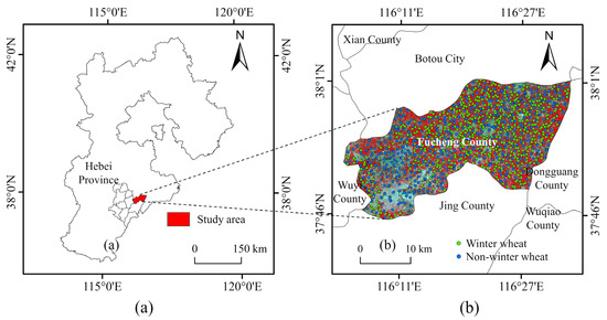
Figure 1.
(a) Location of the study area, (b) the spatial distribution of sample data.
2.2. Remote Sensing Data
Sentinel-2 is a type of high-resolution multispectral imaging satellite. There are two Sentinel-2 satellites, 2A and 2B. The revisit period of one satellite is 10 days, while the two satellites complement each other, and the revisit period is five days. Sentinel-2 has different spatial resolutions (10 m, 20 m, and 60 m) from the visible and near-infrared to shortwave infrared bands. In this study, band 4 and band 8 with 10 m resolution were used. According to the principle of low cloud cover (less than 10%) and as consistent an image time interval as possible and in consideration of the winter wheat growth period and phenological characteristics, 21 high-quality Sentinel-2 high-resolution images were selected, which covered the entire growth period of winter wheat from October 2017 to June 2018 (Table 1). These images were downloaded from the United States Geological Survey (https://earthexplorer.usgs.gov/ (accessed on 12 March 2021)). Because the downloaded Sentinel-2 remote sensing images were Level 1C (L1C), radiometric calibration and FLAASH atmospheric correction were carried out to obtain the real surface reflectance data [38]. The input data on FLAASH atmospheric correction were the result of Sentinel-2 L1C radiometric calibration. The data preprocessing of the Sentinel-2 remote sensing images also included mosaic, clipping, and band operations.

Table 1.
List of Sentinel-2 images.
In this study, NDVI time series data were selected to extract the spatial distribution of winter wheat in Fucheng County. The NDVI was calculated, as follows:
where is the reflectance of the near-infrared band and is the reflectance of the red band.
The NDVI time series could be obtained by layering the images in chronological order. However, remote sensing images are easily affected by clouds and aerosols, which could cause abnormal fluctuations in the NDVI time series. Therefore, it was necessary to smooth and denoise the NDVI time series data [39]. In this study, Savitzky-Golay (S-G) filtering was adopted to obtain high-quality NDVI time series data [40]. Figure 2 shows the NDVI time series of winter wheat before and after smoothing.
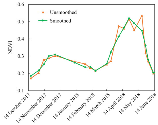
Figure 2.
Normalized difference vegetation index (NDVI) time series of winter wheat before and after smoothing (Location: 37°50′29.73″ N, 116°15′12.75″ E).
2.3. Sampling Point Data
In addition to the 96 ground samples that were obtained from field surveys (comprising 51 winter wheat samples and 45 non-winter wheat samples (of buildings, roads, woodland, and water), 1094 samples were selected from high-resolution Google Earth images. These latter samples included 609 winter wheat samples and 485 non-winter wheat samples. On this basis, 100 winter wheat samples and 90 non-winter wheat samples were randomly selected from the sample data (Figure 1), which were regarded as training samples. The winter wheat training samples were mainly used to extract the reference NDVI time series, and the non-winter wheat training samples were mainly used for the final comparative analysis. The remaining 560 winter wheat samples and 440 non-winter wheat samples were used as verification samples for verifying the crop identification accuracy of the results of crop distribution extraction.
2.4. Other Data
The auxiliary data in this study included the administrative vector data from Fucheng County, official statistical data on the winter wheat planting area, and winter wheat phenology information for Fucheng County in 2018. The statistical data on the winter wheat planting area were used as the reference for the total amount control and then used to verify the total area accuracy of the winter wheat area extraction.
3. Methodology
A variety of similarity measurement methods were selected to carry out comparative studies on the accuracy of winter wheat distribution mapping based on Sentinel-2 NDVI time series data. The workflow consisted of the following steps: (1) obtaining the reference and actual cross-correlation curves according to the multitemporal Sentinel-2 data and the cross correlogram spectral matching (CCSM) algorithm; (2) calculating the similarity between two cross-correlation curves and constructing a winter wheat extraction model according to the similarity; (3) optimizing the threshold value in the winter wheat extraction model using the SCE-UA global optimization algorithm; and, (4) extracting and mapping the spatial distribution of regional winter wheat and performing an accuracy assessment (Figure 3). The similarity measurement indicators included the Manhattan distance (MD), ED, SAM, root mean square error (RMSE), spectral correlation coefficient (SCC), and DTW.
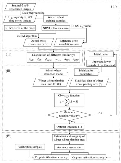
Figure 3.
Flowchart for extracting and mapping winter wheat. (Note: The software ENVI and MATLAB were used in step I; steps II and III were mainly carried out in MATLAB; and in step IV, ENVI, and ArcMap were mainly used.).
3.1. Cross Correlogram Spectral Matching (CCSM) Algorithm
In the CCSM algorithm, the cross-correlation curve was constructed by calculating the cross-correlation coefficients of the reference spectrum curve and the target spectrum curve at different matching positions, and the degree of the match between the reference cross-correlation curve and actual cross-correlation curve was used to describe the similarity of the spectral curves and identify the features [41,42,43]. The specific process of the cross-correlation calculation using NDVI time series in this study is as follows: first, the NDVI time series winter wheat data set was obtained based on the winter wheat training sample data. Subsequently, the NDVI time series reference curve for winter wheat was obtained by averaging the NDVI values of each phase in the NDVI time series winter wheat data set [37]. Finally, according to the CCSM algorithm, the cross-correlation coefficients of the NDVI time series reference curve of winter wheat and the NDVI time series curve of the target pixel at different matching positions were calculated. The cross-correlation coefficient is calculated, as follows:
where r is the NDVI time series reference curve of winter wheat; t is the NDVI time series curve of the target pixel; and are the NDVI values that correspond to the NDVI time series reference curve of winter wheat and the NDVI time series curve of the target pixel, respectively; n is the number of overlapping bands of the two curves after moving; and, m is the movement position of the target pixel NDVI time series curve. M = 0 means no movement, m = −1 means the target curve moves one band position to the left relative to the reference curve, m = 1 means the target curve moves one band position to the right relative to the reference curve, and is the cross-correlation at moving position m.
The cross-correlation coefficient at different moving positions could be drawn as a cross-correlation curve (actual cross-correlation curve). Theoretically, if the crop type does not change, the NDVI time series curve of the target pixel remains consistent with the winter wheat NDVI time series reference curve. At this time, the cross-correlation curve that is obtained from these two curves is the reference cross-correlation curve of winter wheat. Figure 4 shows the reference cross-correlation curve and the actual cross-correlation curve.
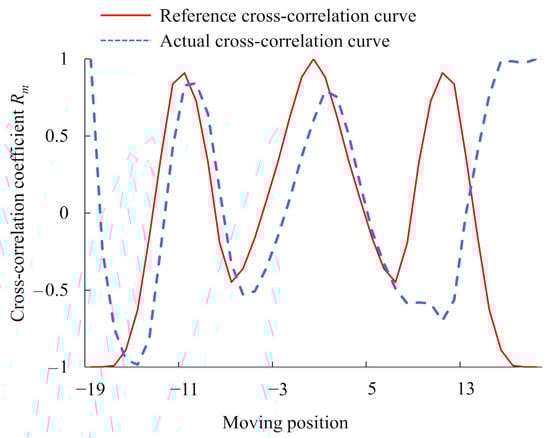
Figure 4.
Reference cross-correlation curve and actual cross-correlation curve (Location: 37°55′9.17″ N, 116°18′4.81″ E).
3.2. Calculation of Different Similarity Indicators
According to the reference cross-correlation curve of winter wheat and the actual cross-correlation curve of the target pixel, six similarity measurement indicators were selected to describe the difference between the two curves: MD, ED, RMSE, SAM, SCC, and DTW.
The MD mainly measures the sum of the absolute wheelbases of two curves in the standard coordinate system: the smaller the MD, the more similar the two curves [44]. The ED mainly refers to the true distance between two points in m-dimensional space; the smaller the ED between two time series, the more similar the two time series are [45,46]. The RMSE is a derivative of the ED; for two curves, the smaller the RMSE value, the more similar the two curves are [43]. SAM uses the standard spectral curve as a reference to calculate the generalized angle between the spectral curve of each pixel in the image and the reference spectral curve; the smaller the angle, the more similar the two curves are [47,48,49]. The SCC mainly uses the correlation to evaluate the similarity of two spectra, with values between −1 and 1; the closer the value is to 1, the more similar the two curves are [44]. The specific calculation formulas for the above similarity measurement indicators are as follows:
where and represent the cross-correlation coefficients of the reference cross-correlation curve and the actual cross-correlation curve at moving position i, respectively; m is the maximum moving position; k is the number of moving positions; and , , , , and represent the MD, ED, RMSE, SAM, and SCC, respectively.
DTW is a widely used algorithm in the extraction of crop spatial distribution [50,51,52]. This algorithm calculates the shortest distance between two time series curves by finding the curved path with the lowest cost, and it is used to measure the similarity between the two time series curves. The DTW algorithm can calculate the DTW distance between two time series curves by extending and shortening time series with different lengths and different starting and ending times. The specific principles are as follows [52]:
Assume that time series ai(t) = {a1, a2, …, am} and bj(t) = {b1, b2, …, bn}, and their lengths are m and n, respectively. Subsequently, an m × n distance matrix Cm × n is constructed, and each element in the matrix cij = d(ai, bj) = is the ED. In the Cm × n distance matrix, a set of continuous matrix elements W = w1, w2, …, wk is defined as a curved path, which must meet the following conditions. (a) Boundary conditions: the first element of the path is w1 = c11, and the last element is wk = cmn. (b) Continuity: the adjacent elements in the path must be continuous; if wk = cij and wk-1 = ci’j’, then i-i’≤1 and j-j’≤1. (c) Monotonicity: the next position of the path does not decrease in the row direction and column direction on the basis of the previous position; if wk = cij and wk-1 = ci’j’, then i-i’≥0 and j-j’≥0. (d) Boundedness: the number of matrix elements passed by the path has upper and lower limits, which is, max(m, n) ≤ k ≤ (m+n−1). The main idea of the DTW algorithm is to find a path with the smallest bending cost:
where i = 2, 3, …, m; j = 2, 3, …, n; the DTW distance of the two time series curves is given by the minimum cumulative value w(m, n) of the curved path. The smaller the DTW distance, the more similar the two time series curves.
3.3. Establishment of the Winter Wheat Extraction Model
The similarity between the reference cross-correlation curve and the actual cross-correlation curve could be calculated by the MD, ED, RMSE, SAM, SCC, and DTW.
According to the different similarity calculation results, the smaller the , , , , and values, the more similar the actual cross-correlation curve and the reference cross-correlation curve, and the greater the probability that the pixel is winter wheat. Therefore, when these similarities are within a certain range, the ground feature type that is represented by the target pixel can be identified as winter wheat, and the winter wheat spatial distribution extraction model is established, as follows:
However, for the similarity result that is calculated by SCC, the greater the value, the more similar the actual cross-correlation curve and the reference cross-correlation curve. Therefore, the winter wheat spatial distribution extraction model is as follows:
where represents the value of the i-th row and j-th column in the image; 1 means winter wheat, 0 means non-winter wheat; represents the calculated similarities of the pixel in the i-th row and j-th column in the image, such as , , , , and ; Q represents MD, ED, RMSE, SAM, and DTW; represents the similarity of the pixel in the i-th row and j-th column calculated by SCC; and, T is the corresponding threshold in the winter wheat extraction model under different similarities, which is the parameter to be optimized in this paper.
3.4. Optimization of the Threshold in the Extraction Model
In this study, to automatically optimize the threshold in the crop extraction model that is based on the similarity of NDVI time series curve, extract a highly accurate crop area distribution, and obtain mapping results that are consistent with the crop area statistical data, the statistical data on the regional winter wheat planting area were used for external optimization data comparison. Based on the establishment of the cost function between the regional remote sensing-based crop area extraction results and the crop area statistical data, the SCE-UA global optimization algorithm was used to obtain the optimal threshold of the winter wheat extraction model. The optimal threshold value of the winter wheat extraction model was obtained when the difference between the extracted regional winter wheat planting area and the winter wheat planting area statistical data was the smallest. Subsequently, the extracted spatial distribution of winter wheat was output under this optimal threshold.
The SCE-UA algorithm is a global optimization algorithm that was proposed by Duan et al. [53]. This algorithm combines the advantages of deterministic search, random search, and evolutionary algorithms, and it has strong global search capabilities and high convergence speed and processing efficiency. This algorithm is also one of the most effective methods for finding the optimal value for nonlinear complex models [54,55]. The specific process of threshold optimization using the SCE-UA algorithm in this study is as follows:
(1) Determine the upper and lower bounds of the threshold in the winter wheat distribution extraction model. In the model for the extraction of the winter wheat spatial distribution, the upper bound of the threshold was set to the maximum value of the similarities in the winter wheat training samples, and the lower bound of the threshold was set to 0, as shown in Formula (9). In the model for the extraction of the winter wheat spatial distribution, the upper bound of the threshold was set to 1, and the lower bound was set to the minimum value of the SCC in the winter wheat training samples, as shown in Formula (10). The initial value of the threshold was set as the average value of the similarity in the winter wheat training samples.
(2) Determine the main parameters of the SCE-UA algorithm. In the SCE-UA algorithm, the values of most of the parameters, such as β = 2n + 1, m = 2n + 1, α = 1, and q = n + 1, were mainly set to the default values of the algorithm itself. Here, β is the number of evolution steps that were taken by each complex; m is the number of points in a complex; α is the number of consecutive offspring generated by each subcomplex; q is the number of points in a subcomplex; and, n is the dimensions of the problem, in this paper, n = 1. The number of complexes p is the only parameter that needs to be determined; this parameter needs to be determined in consideration of specific problems. If the number of complexes is high, the amount of calculation will be increased; if the number of complexes is low, the optimization effect will not be achieved. In this study, we set p = 2.
(3) Establishment of objective function. Supported by the SCE-UA algorithm, the statistical data on the regional winter wheat planting area were used as the reference for total amount control. Combined with the remote sensing extraction results of the winter wheat planting area, the objective function was established, as follows:
where y is the sum of the difference between the remote sensing extraction results of the regional winter wheat planting area and the statistical data on crop planting area (total amount control data); E is the total area of winter wheat that is extracted by remote sensing; S is the statistical data on the winter wheat planting area; and, n is the number of study areas (here n = 1).
(4) Determine the iteration stop rule. The optimization will be stopped when one of the following three conditions occurs during the optimization process: (a) the objective function value cannot be significantly ameliorated; (b) the maximum number of iterations of the objective function exceeds 10,000; and, (c) the threshold to be optimized exhibits no significant change after five consecutive iterations. At this time, the objective function reaches the optimal state, the iteration is stopped, and the optimal threshold is output.
3.5. Accuracy Assessment of Crop Mapping Results
In order to evaluate the accuracy of the spatial distribution extraction results of winter wheat and the degree of consistency with the statistical data on crop planting area, the accuracy evaluation of the crop area extraction and mapping results from the WWM-SMITO method is mainly verified from two aspects: crop identification accuracy (i.e., location accuracy) and crop area estimation accuracy (i.e., total area accuracy) [56]. The crop identification accuracy was mainly used to evaluate the accuracy of the crop spatial distribution extraction results, and the indicators mainly included the overall accuracy (OA), kappa coefficient (kappa), producer accuracy (PA), and user accuracy (UA), which were obtained in the confusion matrix [57,58]. The OA and kappa values are both between 0 and 1, and the closer the value is to 1, the higher the accuracy of the crop distribution extraction. PA and UA indicate the classification accuracy of a single category. In addition, when compared with crop area statistical data, the crop area estimation accuracy was mainly used to evaluate the total area accuracy. The specific total area accuracy was calculated, as follows:
where TA is the total crop area accuracy (%); E is the area of winter wheat extracted by remote sensing (m2); and, S is the statistical data on the winter wheat planting area in the study area (m2).
4. Results and Analysis
4.1. The Results of Different Similarity Indicators
The similarity between the winter wheat reference cross-correlation curve and the actual cross-correlation curve of the target pixel was calculated, according to the formulas used to calculate the different similarity measurement indicators. Figure 5 shows the spatial distribution of each indicator. The principles of the different similarity measurement methods were combined, and the smaller the MD, ED, RMSE, SAM, and DTW similarity values and the greater the SCC similarity values were, the higher the probability that the pixel belonged to winter wheat. Depending on the ground survey sample points, 40 samples were selected from four types of non-winter wheat training samples: buildings, woodland, water, and winter wheat. Then, the average similarities of these four types of ground objects under different similarity indicators were calculated and they are shown in Figure 6 using a histogram. The similarity between winter wheat and other ground objects (such as buildings, woodland, and water) was quite different when the same similarity indicator was used, as shown in Figure 6. Because the cross-correlation curves of winter wheat pixels were very similar to the reference cross-correlation curves of winter wheat, the values of MD, ED, RMSE, SAM, and DTW were very low, and the SCC values were very high. In contrast, the cross-correlation curves of non-winter wheat pixels were very different from the reference cross-correlation curves of winter wheat, so the MD, ED, RMSE, SAM, and DTW values were very high, and the SCC values were very low. These properties were conducive to the optimization of the similarity threshold to extract the spatial distribution of winter wheat.
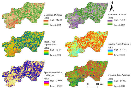
Figure 5.
Calculation results of different similarity indicators.
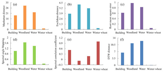
Figure 6.
Average similarity of each land cover type with different indicators: (a) MD, (b) ED, (c) RMSE, (d) SAM, (e) SCC, (f) DTW.
4.2. Threshold Optimization Results of the Winter Wheat Extraction Model
On the basis of obtaining different similarities, the statistical data on the winter wheat planting area in Fucheng County were used as the object for the comparison of external optimization data, and the average similarity of winter wheat training samples was used as the initial threshold. The SCE-UA algorithm was used to optimize the thresholds of the winter wheat extraction models under the conditions of different similarity indicators. Finally, the optimal threshold values of the model for the extraction of the spatial distribution of winter wheat with different similarities in the study area in 2018 were obtained (Table 2). The difference between the remote sensing extraction results of winter wheat in Fucheng County using the optimal threshold and the statistical data on the county-level winter wheat planting area was minimized, as shown in Table 2. Among them, the minimum objective function values of MD, ED, RMSE, and DTW were 0, and the minimum objective function values of SAM and SCC were only 100 m2. These results indicated that the method proposed for regional winter wheat extraction and mapping based on the threshold optimization of the NDVI time series similarity in this study could ensure high consistency between the regional crop area that was extracted by remote sensing and the regional crop area statistical data.
Table 2.
Optimization of threshold parameters of the winter wheat extraction model.
4.3. Extraction Results of Winter Wheat Spatial Distribution and Their Verification
According to the optimal thresholds of the winter wheat extraction models under different similarity indicators, the spatial distributions of winter wheat in Fucheng County were extracted, and Figure 7 shows the results. The winter wheat in Fucheng County was mainly distributed in the central and eastern parts of this county, but the western part was urban areas, where winter wheat was less distributed, as shown in Figure 7.
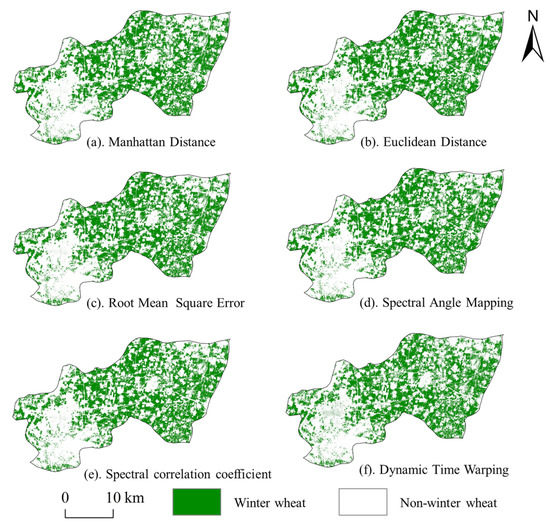
Figure 7.
Extraction and mapping results of winter wheat using different similarity indicators, (a) MD, (b) ED, (c) RMSE, (d) SAM, (e) SCC, (f) DTW.
Table 3 lists the accuracies of the winter wheat results extracted by different similarity indicators. There was little difference between the winter wheat area statistical data and the winter wheat planting area extracted under the optimal threshold with different similarity indicators. The winter wheat planting area in Fucheng County that was obtained by MD, ED, RMSE, and DTW was 289,196,000 m2, which was the same as the winter wheat area statistical data for Fucheng County, and the total area accuracy reached 100%. Moreover, the winter wheat planting area in Fucheng County that was obtained by the SAM and SCC indicators was 289,195,900 m2, and the difference was only 100 m2 when compared with the statistical data on the winter wheat area in Fucheng County, and the total area accuracy was 99.99%. This result indicated that using the SCE-UA algorithm to set the threshold could ensure the accuracy and high precision of the winter wheat area extraction and achieve close agreement between the crop area statistics and the crop area extracted by remote sensing.
Table 3.
Optimization of the threshold parameters of the winter wheat extraction model.
Moreover, depending on the verification sample data, the six winter wheat extraction results based on time series similarity were evaluated with four accuracy indicators: overall classification accuracy, kappa coefficient, PA, and UA. Under the condition of ensuring high total area accuracy, the identification accuracy of the regional winter wheat extraction results using different similarity indicators reached high levels, as shown in Table 3. The OA of the mapping results from the RMSE similarity indicator was 94.5%, and the kappa coefficient was 0.8894. The overall accuracies of the area extraction results of winter wheat using the similarity of ED, MD, SAM, and SCC were 94.1%, 93.9%, 93.3%, and 92.8%, respectively. Among the indicators, DTW yielded the lowest extraction accuracy; however, the OA and kappa coefficient were 86.2% and 0.7256, respectively, indicating that the indicator could meet the general requirements regarding the accuracy of regional remote sensing-based crop area extraction.
The OA of the mapping results from the six different similarity indicators in descending order was RMSE>ED>MD>SAM>SCC>DTW. The differences in OA between RMSE and ED, MD, SAM, SCC, and DTW were 0.4%, 0.6%, 1.2%, 1.7%, and 8.3%, respectively. As the difference between the indicators was within 1%, the mapping results of RMSE were similar to those of the ED and MD similarity indicators. The differences in OA between the RMSE and the SAM and SCC were within 2%. Additionally, the mapping results of the DTW indicator were obviously different from those of the other indicators. The reason for this difference might be that the DTW indicator did not require a one-to-one correspondence between the matching points, and it only needed the smallest accumulated distance between the two matched sequences, which might cause malformed matching and ultimately affect the crop extraction accuracy.
5. Discussion
5.1. Total Amount Control of Crop Area Statistics
The proposed WWM-SMITO method achieved the high-precision extraction of winter wheat spatial distribution in Fucheng county. In this study, the regional winter wheat planting area statistics were used as reference data. When the difference between the winter wheat planting area extracted by remote sensing and the statistical data on the regional winter wheat planting area was smallest, the optimal threshold (T) of the crop extraction model was obtained in order to extract the regional winter wheat spatial distribution. The verification results showed that the spatial distribution of regional crop area that was extracted by the proposed WWM-SMITO method not only achieved a high total area accuracy (more than 99.99%) and high consistency with the crop area statistical data, but also high crop identification accuracy. Most of the studies on crop distribution extraction and crop mapping have not considered crop area statistics in the process of crop area extraction, but have only verified the accuracy of the extraction results through comparison with statistical data [15,16,17]. Among those studies that have considered crop area statistics during crop area extraction, statistical data were not used as a total control parameter [24,25,26,27]. Therefore, the total area accuracy of the crop mapping results of prior studies needs to be improved.
The overall accuracy and total area accuracy of the proposed WWM-SMITO method were improved when compared with those of previous methods; the total area accuracy was improved by approximately 4.89–23% [15,16,17,34]. The proposed WWM-SMITO method achieved good performance in winter wheat mapping under the condition of total amount control of crop area statistics. Therefore, the proposed research method could provide a reference for the spatialization of regional crop area statistical data and for downscaling the reconstruction of long-term statistical data on crop areas over large-scale regions.
5.2. Threshold Optimization of the Crop Extraction Model
In research on crop planting area recognition, a threshold model is frequently used to extract crop distribution information. Threshold setting is an important problem in the threshold method [59]. In most traditional threshold methods, in order to obtain a group of thresholds with high classification accuracy, the threshold parameters of the key phenological periods need to be manually adjusted many times [60]. In recent years, a series of studies on reasonable threshold setting have been carried out [61,62], but the automation of threshold setting still needs improvement. In this study, the SCE-UA global optimization algorithm was used to realize the automatic optimization of the threshold in the winter wheat extraction model, which not only avoided the time-consuming manual adjustment of parameters, but also improved the accuracy of crop distribution extraction and mapping. Thus, the method of automatic optimization of threshold model parameters that was used in this study could provide a foundation for future applications of the proposed WWM-SMITO method to extract the crop distribution information in larger regions.
5.3. Shortcomings and Suggestions for Improvement
Although good performance was achieved in this study, some shortcomings still need to be further improved. First, this research did not use cultivated land as mask data to extract the winter wheat planting area. In follow-up studies, cultivated land data could be used to mask the non-cultivated land information to evaluate the impacts of a cultivated land mask on crop distribution mapping. Second, the present research on crop area extraction and mapping was only conducted in the main winter wheat production area in China, and only winter wheat was considered to be the research crop. In our next steps, crop distribution extraction and mapping of different crops growing in the same growing season (such as corn, soybean, and cotton) with complex planting structures will be considered at larger scales, such as the municipal and provincial levels. Third, a comparative study of the accuracy of the crop area extraction and mapping of six similarity indicators was carried out, and the crop area extraction accuracy of each indicator was ranked. However, whether this precision order is suitable for other crops and regions requires further research. Finally, in this paper, the selected feature parameters were single, and only NDVI time series data were used to extract and map the winter wheat area. In the future, it will be necessary to introduce other remote sensing parameters (such as the enhanced vegetation index (EVI) and other vegetation indices, spectral features, and texture features) for research on crop spatial distribution mapping that is based on the threshold optimization of the similarity of time series curves.
6. Conclusions
Fucheng County of Hebei Province in the Huanghuaihai Plain of China was taken as the study area to obtain high-precision information on the crop spatial distribution consistent with crop planting area statistics. Sentinel-2 NDVI time series data were used, and the spatial distribution information for winter wheat was extracted based on different similarity measurement indicators and their optimized thresholds. The main conclusions are as follows:
(1) With the support of the SCE-UA global optimization algorithm, which was based on the total amount control of statistical data and threshold optimization of NDVI time series similarity, the WWM-SMITO method for extracting and mapping the winter wheat distribution was proposed in this study. The verification results showed that the total area accuracy and identification accuracy of the regional winter wheat distribution extraction results that were obtained by this proposed method reached a high level. These results ensured not only that the area of winter wheat extracted by remote sensing was highly consistent with the statistical data, but also that the identification accuracy of the winter wheat extraction results could meet the accuracy requirements of users. Using the method that was proposed in this research, the regional winter wheat area extracted by remote sensing and crop area statistical data were unified, and the proposed method was proven to have certain validity and feasibility.
(2) Based on six different similarity indicators, ED, MD, SAM, SCC, RMSE, and DTW, crop area statistical data were regarded as reference for the winter wheat planting area that was extracted by remote sensing, the spatial distribution of winter wheat was extracted based on similarity threshold optimization, and their accuracies were compared. The results showed that the identification accuracy of winter wheat extracted by using the RMSE indicator was the highest, of which the OA was 94.5% and the kappa coefficient was 0.8894. The overall accuracies of winter wheat extraction based on ED, MD, SAM, and SCC indicators were 94.1%, 93.9%, 93.3%, and 92.8%, respectively, and the kappa coefficients were 0.8815, 0.8776, 0.8657, and 0.8558, respectively. The accuracy of the winter wheat mapping results that were extracted by DTW was the lowest, with an OA of 86.2% and a kappa coefficient of 0.7256. The above results could provide certain guidance for the selection of the similarity index in the extraction and mapping of winter wheat based on the similarity of time series vegetation index curves.
Author Contributions
Conceptualization, J.R.; methodology, J.R. and F.L.; software, F.L.; validation, F.L., H.Z. and N.Z.; formal analysis, F.L. and S.W.; investigation, all authors; resources, J.R., S.W. and H.Z.; data curation, F.L.; writing—original draft preparation, F.L.; writing—review and editing, all authors; visualization, F.L.; supervision, J.R.; project administration, J.R.; funding acquisition, J.R. All authors have read and agreed to the published version of the manuscript.
Funding
This research was funded by the National Natural Science Foundation of China (41871353, 41801286, 41471364, 61661136006), the Young Elite Scientists Sponsorship Program by CAST (2018CAASS04), the Fundamental Research Funds for Central Nonprofit Scientific Institution (1610132021009), and the Agricultural Science and Technology Innovation Program of the Chinese Academy of Agricultural Sciences.
Acknowledgments
The authors would like to thank USGS for providing Sentinel-2 data. We are thankful to the editors and the three anonymous reviewers for their constructive comments and suggestions that significantly improve the quality of the manuscript.
Conflicts of Interest
The authors declare no conflict of interest.
References
- Barnwal, P.; Kotani, K. Climatic impacts across agricultural crop yield distributions: An application of quantile regression on rice crops in Andhra Pradesh, India. Ecol. Econ. 2013, 87, 95–109. [Google Scholar] [CrossRef]
- Feng, L.; Jia, Z.; Zhang, J. The dynamic monitoring of corn planting area distribution in response to climate change from 2001 to 2010: A case study of Northeast China. Geogr. Tidsskr. -Dan. J. Geogr. 2016, 116, 44–55. [Google Scholar] [CrossRef]
- Dempewolf, J.; Adusei, B.; Becker-Reshef, I.; Hansen, M.; Potapov, P.; Khan, A.; Barker, B. Wheat Yield Forecasting for Punjab Province from Vegetation Index Time Series and Historic Crop Statistics. Remote Sens. 2014, 6, 9653–9675. [Google Scholar] [CrossRef]
- Gallego, F.J.; Stibig, H.J. Area estimation from a sample of satellite images: The impact of stratification on the clustering efficiency. Int. J. Appl. Earth Obs. Geoinf. 2013, 22, 139–146. [Google Scholar] [CrossRef]
- Khan, A.; Hansen, M.; Potapov, P.; Adusei, B.; Pickens, A.; Krylov, A.; Stehman, S.V. Evaluating Landsat and RapidEye Data for Winter Wheat Mapping and Area Estimation in Punjab, Pakistan. Remote Sens. 2018, 10, 489. [Google Scholar] [CrossRef]
- Liu, J.; Zhu, W.; Atzberger, C.; Zhao, A.; Pan, Y.; Huang, X. A Phenology-Based Method to Map Cropping Patterns under a Wheat-Maize Rotation Using Remotely Sensed Time-Series Data. Remote Sens. 2018, 10, 1203. [Google Scholar] [CrossRef]
- Song, Y.; Wang, J. Mapping Winter Wheat Planting Area and Monitoring Its Phenology Using Sentinel-1 Backscatter Time Series. Remote Sens. 2019, 11, 449. [Google Scholar] [CrossRef]
- Li, F.; Qin, Q.; Wang, H.; Hu, X.; Zhao, H. Extraction of Planting Information of Winter Wheat in a Province Based on GF-1/WFV Images. Meteor Environ. Res. 2018, 9, 100–105. [Google Scholar] [CrossRef]
- Wang, J.; Liu, J.; Zhuan, D.; Li, L.; Ge, Y. Spatial sampling design for monitoring the area of cultivated land. Int. J. Remote Sens. 2002, 23, 263–284. [Google Scholar] [CrossRef]
- Wu, M.; Yang, L.; Yu, B.; Wang, Y.; Zhao, X.; Niu, Z.; Wang, C. Mapping crops acreages based on remote sensing and sampling investigation by multivariate probability proportional to size. Trans. Chin. Soc. Agric. Eng. 2014, 30, 146–152. (In Chinese) [Google Scholar] [CrossRef]
- Gandharum, L.; Mulyani, M.E.; Hartono, D.M.; Karsidi, A.; Ahmad, M. Remote sensing versus the area sampling frame method in paddy rice acreage estimation in Indramayu regency, West Java province, Indonesia. Int. J. Remote Sens. 2021, 42, 1738–1767. [Google Scholar] [CrossRef]
- Zhang, J.; Pan, Y.; Hu, T.G.; Chen, L.; Dong, Y. Analysis of influence factors about space sampling efficiency of winter wheat planting area. Trans. Chin. Soc. Agric. Eng. 2009, 25, 169–173. (In Chinese) [Google Scholar] [CrossRef]
- Zhang, H.; Li, Q.; Wen, N.; Du, X.; Tao, Q.; Dong, T. Analysis on estimation accuracy of crop area caused by spatial sampling factors based on remote sensing data. Trans. Chin. Soc. Agric. Eng. 2014, 30, 176–184. (In Chinese) [Google Scholar] [CrossRef]
- Tan, J.; Zhang, J.; Gao, C.; Bao, Y. Winter wheat area estimation based on structure and scale using remote sensing. Trans. Chin. Soc. Agric. Eng. 2012, 28, 114–122. (In Chinese) [Google Scholar] [CrossRef]
- Wei, M.; Qiao, B.; Zhao, J.; Zuo, X. The area extraction of winter wheat in mixed planting area based on Sentinel-2 a remote sensing satellite images. Int. J. Parallel. Emerg. Distrib. Syst. 2020, 35, 297–308. [Google Scholar] [CrossRef]
- Liu, X.; Li, F.; Guo, L. Winter Wheat Planting Information Extraction in Qingdao: Based on High-resolution Satellite Imagery. Chin. Agric. Sci. Bull. 2020, 36, 118–123. (In Chinese) [Google Scholar]
- Yang, H.; Deng, F.; Zhang, J.; Wang, X.; Ma, Q.; Xu, N. A study of information extraction of rape and winter wheat planting in Jianghan Plain based on MODIS EVI. Remote Sens. Land Resour. 2020, 32, 208–215. (In Chinese) [Google Scholar] [CrossRef]
- He, H.; Zhu, X.; Pan, Y.; Zhu, W.; Zhang, J.; Jia, B. Study on Scale Issues in Measurement of Winter Wheat Plant Area by Remote Sensing. J. Remote Sens. 2008, 12, 168–175. (In Chinese) [Google Scholar] [CrossRef]
- Abdikan, S.; Sanli, F.B.; Sunar, F.; Ehlers, M. A comparative data-fusion analysis of multi-sensor satellite images. Int. J. Digit. Earth 2014, 7, 671–687. [Google Scholar] [CrossRef]
- Zhang, W.; Li, A.; Jin, H.; Bian, J.; Zhang, Z.; Lei, G.; Qin, Z.; Huang, C. An Enhanced Spatial and Temporal Data Fusion Model for Fusing Landsat and MODIS Surface Reflectance to Generate High Temporal Landsat-Like Data. Remote Sens. 2013, 5, 5346–5368. [Google Scholar] [CrossRef]
- Esch, T.; Metz, A.; Marconcini, M.; Keil, M. Combined use of multi-seasonal high and medium resolution satellite imagery for parcel-related mapping of cropland and grassland. Int. J. Appl. Earth Obs. Geoinf. 2014, 28, 230–237. [Google Scholar] [CrossRef]
- Van Dijk, M.; You, L.; Havlik, P.; Mosnier, A. Generating high-resolution national crop distribution maps: Combining statistics, gridded data and surveys using an optimization approach. In Proceedings of the International Association of Agricultural Economists 2018 Conference, Vancouver, BC, Canada, 28 July–2 August 2018. [Google Scholar]
- Lu, J.; Huang, J.; Wang, L.; Pei, Y. Paddy rice planting information extraction based on spatial and temporal data fusion approach in Jianghan Plain. Resour. Environ. Yangtze Basin. 2017, 26, 874–881. (In Chinese) [Google Scholar] [CrossRef]
- Tan, J.; Yang, P.; Liu, Z.; Wu, W.; Zhang, L.; Li, Z.; You, L.; Tang, H.; Li, Z. Spatio-temporal dynamics of maize cropping system in Northeast China between 1980 and 2010 by using spatial production allocation model. J. Geogr. Sci. 2014, 24, 397–410. [Google Scholar] [CrossRef]
- Xia, T.; Wu, W.; Zhou, Q.; Zhou, Y.; Luo, J.; Yang, P.; Li, Z. Spatialization of Statistical Crop Planting Area Based on Geographical Regression. J. Nat. Resour. 2016, 31, 1773–1782. (In Chinese) [Google Scholar] [CrossRef]
- You, L.; Wood, S.; Wood-Sichra, U. Generating plausible crop distribution maps for Sub-Saharan Africa using a spatially disaggregated data fusion and optimization approach. Agric. Syst. 2009, 99, 126–140. [Google Scholar] [CrossRef]
- Lu, M.; Wu, W.; You, L.; Chen, D.; Zhang, L.; Yang, P.; Tang, H. A Synergy Cropland of China by Fusing Multiple Existing Maps and Statistics. Sensors 2017, 17, 1613. [Google Scholar] [CrossRef]
- Li, Q.; Wang, C.; Zhang, B.; Lu, L. Object-Based Crop Classification with Landsat-MODIS Enhanced Time-Series Data. Remote Sens. 2015, 7, 16091–16107. [Google Scholar] [CrossRef]
- Pan, Y.; Li, L.; Zhang, J.; Liang, S.; Hou, D. Crop area estimation based on MODIS-EVI time series according to distinct characteristics of key phenology phasesa case study of winter wheat area estimation in small-scale area. J. Remote Sens. 2011, 15, 578–594. [Google Scholar] [CrossRef]
- Singha, M.; Wu, B.; Zhang, M. Object-Based Paddy Rice Mapping Using HJ-1A/B Data and Temporal Features Extracted from Time Series MODIS NDVI Data. Sensors 2017, 17, 10. [Google Scholar] [CrossRef]
- Zhu, C.; Lu, D.; Victoria, D.; Dutra, L.V. Mapping Fractional Cropland Distribution in Mato Grosso, Brazil Using Time Series MODIS Enhanced Vegetation Index and Landsat Thematic Mapper Data. Remote Sens. 2015, 8, 22. [Google Scholar] [CrossRef]
- Gao, H.; Wang, C.; Wang, G.; Li, Q.; Zhu, J. A New Crop Classification Method Based on the Time-Varying Feature Curves of Time Series Dual-Polarization Sentinel-1 Data Sets. IEEE Geosci. Remote Sens. Lett. 2020, 17, 1183–1187. [Google Scholar] [CrossRef]
- Sun, H.; Xu, A.; Lin, H.; Zhang, L.; Mei, Y. Winter wheat mapping using temporal signatures of MODIS vegetation index data. Int. J. Remote Sens. 2012, 33, 5026–5042. [Google Scholar] [CrossRef]
- Yang, Y.; Tao, B.; Ren, W.; Zourarakis, D.P.; Masri, B.E.; Sun, Z.; Tian, Q. An Improved Approach Considering Intraclass Variability for Mapping Winter Wheat Using Multitemporal MODIS EVI Images. Remote Sens. 2019, 11, 1191. [Google Scholar] [CrossRef]
- Dong, Q.; Chen, X.; Chen, J.; Zhang, C.; Liu, L.; Cao, X.; Zang, Y.; Zhu, X.; Cui, X. Mapping Winter Wheat in North China Using Sentinel 2A/B Data: A Method Based on Phenology-Time Weighted Dynamic Time Warping. Remote Sens. 2020, 12, 1274. [Google Scholar] [CrossRef]
- Yonezawa, C. Maximum likelihood classification combined with spectral angle mapper algorithm for high resolution satellite imagery. Int. J. Remote Sens 2007, 28, 3729–3737. [Google Scholar] [CrossRef]
- Guo, Y.; Liu, Q.; Liu, G.; Huang, C. Extraction of Main Crops in Yellow River Delta Based on MODIS NDVI Time Series. J. Nat. Resour. 2017, 32, 1808–1818. (In Chinese) [Google Scholar] [CrossRef]
- Main-Knorn, M.; Pflug, B.; Louis, J.; Debaecker, V. Sen2Cor for Sentinel-2. In Proceedings of the SPIE Remote Sensing, Warschau, Poland, 11–14 September 2017; p. 1042704. [Google Scholar] [CrossRef]
- Hird, J.N.; Mcdermid, G.J. Noise reduction of NDVI time series: An empirical comparison of selected techniques. Remote Sens. Environ. 2009, 113, 248–258. [Google Scholar] [CrossRef]
- Chen, J.; Jönsson, P.; Tamura, M.; Gu, Z.; Matsushita, B.; Eklundh, L. A simple method for reconstructing a high-quality NDVI time-series data set based on the Savitzky–Golay filter. Remote Sens. Environ. 2004, 91, 332–344. [Google Scholar] [CrossRef]
- Van Der Meer, F.; Bakker, W. Cross correlogram spectral matching Application to surface mineralogical mapping by using AVIRIS data from Cuprite, Nevada. Remote Sens. Environ. 1997, 61, 371–382. [Google Scholar] [CrossRef]
- Van Der Meer, F.; Bakker, W. CCSM: Cross correlogram spectral matching. Int. J. Remote Sens. 2010, 18, 1197–1201. [Google Scholar] [CrossRef]
- Wang, L.; Chen, J.; Gong, P.; Shimazaki, H.; Tamura, M. Land cover change detection with a cross-correlogram spectral matching algorithm. Int. J. Remote Sens. 2010, 30, 3259–3273. [Google Scholar] [CrossRef]
- Erudel, T.; Fabre, S.; Houet, T.; Mazier, F.; Briottet, X. Criteria Comparison for Classifying Peatland Vegetation Types Using In Situ Hyperspectral Measurements. Remote Sens. 2017, 9, 748. [Google Scholar] [CrossRef]
- Da Silva, M.R.; de Carvalho, O.A., Jr.; Guimarães, R.F.; Gomes, R.A.T.; Silva, C.R. Wheat planted area detection from the MODIS NDVI time series classification using the nearest neighbour method calculated by the Euclidean distance and cosine similarity measures. Geocarto Int. 2020, 35, 1400–1414. [Google Scholar] [CrossRef]
- Ghiyamat, A.; Shafri, H.Z.M.; Mahdiraji, G.A.; Shariff, A.R.M.; Mansor, S. Hyperspectral discrimination of tree species with different classifications using single- and multiple-endmember. Int. J. Appl. Earth Obs. Geoinf. 2013, 23, 177–191. [Google Scholar] [CrossRef]
- Chauhan, H.J.; Buddhiraju, K.M. Effectiveness of Spectral Similarity Measures to Develop Precise Crop Spectra for Hyper-spectral Data Analysis. ISPRS Ann. Photogramm. Remote Sens. Spatial Inf. Sci. 2014, 2, 83–90. [Google Scholar] [CrossRef]
- Yagoub, H.; Belbachir, A.H.; Benabadji, N. Detection and mapping vegetation cover based on the Spectral Angle Mapper algorithm using NOAA AVHRR data. Adv. Space Res. 2014, 53, 1686–1693. [Google Scholar] [CrossRef]
- Abade, N.A.; Júnior, O.A.d.C.; Guimarães, R.F.; De Oliveira, S.N. Comparative Analysis of MODIS Time-Series Classification Using Support Vector Machines and Methods Based upon Distance and Similarity Measures in the Brazilian Cerrado-Caatinga Boundary. Remote Sens. 2015, 7, 12160–12191. [Google Scholar] [CrossRef]
- Guo, Z.; Yang, K.; Liu, C.; Lu, X.; Cheng, L.; Li, M. Mapping National-Scale Croplands in Pakistan by Combining Dynamic Time Warping Algorithm and Density-Based Spatial Clustering of Applications with Noise. Remote Sens. 2020, 12, 3644. [Google Scholar] [CrossRef]
- Guan, X.; Huang, C.; Liu, G.; Meng, X.; Liu, Q. Mapping Rice Cropping Systems in Vietnam Using an NDVI-Based Time-Series Similarity Measurement Based on DTW Distance. Remote Sens. 2016, 8, 19. [Google Scholar] [CrossRef]
- Csillik, O.; Belgiu, M.; Asner, G.P.; Kelly, M. Object-Based Time-Constrained Dynamic Time Warping Classification of Crops Using Sentinel-2. Remote Sens. 2019, 11, 1257. [Google Scholar] [CrossRef]
- Duan, Q.; Gupta, V.K.; Sorooshian, S. Shuffled Complex Evolution Approach for Effective and Efficient Global Minimization. J. Optim. Theory Appl. 1993, 76, 501–502. [Google Scholar] [CrossRef]
- Duan, Q.; Sorooshian, S.; Gupta, V.K. Optimal use of the SCE-UA global optimization method for calibrating watershed models. J. Hydrol. 1994, 158, 265–284. [Google Scholar] [CrossRef]
- Huang, L.; Wang, L.; Zhang, Y.; Xing, L.; Hao, Q.; Xiao, Y.; Yang, L.; Zhu, H. Identification of Groundwater Pollution Sources by a SCE-UA Algorithm-Based Simulation/Optimization Model. Water 2018, 10, 193. [Google Scholar] [CrossRef]
- Zhang, H.; Li, Q. Effects of Spatial Resolution on Crop Identification and Acreage Estimation. Remot Sens. Inf. 2014, 29, 36–40. (In Chinese) [Google Scholar] [CrossRef]
- Congalton, R.G. A review of assessing the accuracy of classifications of remotely sensed data. Remote Sens. Environ. 1991, 37, 35–46. [Google Scholar] [CrossRef]
- Xu, F.; Li, Z.; Zhang, S.; Huang, N.; Quan, Z.; Zhang, W.; Liu, X.; Jiang, X.; Pan, J.; Prishchepov, A.V. Mapping Winter Wheat with Combinations of Temporally Aggregated Sentinel-2 and Landsat-8 Data in Shandong Province, China. Remote Sens. 2020, 12, 2065. [Google Scholar] [CrossRef]
- Wang, M.; Zhang, X.; Huang, Y.; Hong, C.; Zhang, Z.; Huang, X.; Zeng, J.; Tang, J.; Zhang, R. Monitoring of Winter Wheat and Summer Corn Phenology in Xiong’an New Area Based on NDVI Time Series. In Proceedings of the 2019 International Conference on Wireless Communication, Network and Multimedia Engineering (WCNME 2019), Guilin, China, 21 April 2019. [Google Scholar]
- Wang, L.; Liu, J.; Yang, G.; Fu, C.; Teng, F.; Gao, J. Early recognition of winter wheat area based on GF-1 satellite. Trans. Chin. Soc. Agric. Eng. 2015, 31, 194–201. (In Chinese) [Google Scholar] [CrossRef]
- Xun, L.; Zhang, J.; Cao, D.; Wang, J.; Zhang, S.; Yao, F. Mapping cotton cultivated area combining remote sensing with a fused representation-based classification algorithm. Comput. Electron. Agric. 2021, 181, 105940. [Google Scholar] [CrossRef]
- Zhang, J.; Feng, L.; Yao, F. Improved maize cultivated area estimation over a large-scale combining MODIS–EVI time series data and crop phenological information. ISPRS J. Photogramm. Remote Sens. 2014, 94, 102–113. [Google Scholar] [CrossRef]


Publisher’s Note: MDPI stays neutral with regard to jurisdictional claims in published maps and institutional affiliations. |
© 2021 by the authors. Licensee MDPI, Basel, Switzerland. This article is an open access article distributed under the terms and conditions of the Creative Commons Attribution (CC BY) license (http://creativecommons.org/licenses/by/4.0/).