Abstract
In order to acquire a high resolution multispectral (HRMS) image with the same spectral resolution as multispectral (MS) image and the same spatial resolution as panchromatic (PAN) image, pansharpening, a typical and hot image fusion topic, has been well researched. Various pansharpening methods that are based on convolutional neural networks (CNN) with different architectures have been introduced by prior works. However, different scale information of the source images is not considered by these methods, which may lead to the loss of high-frequency details in the fused image. This paper proposes a pansharpening method of MS images via multi-scale deep residual network (MSDRN). The proposed method constructs a multi-level network to make better use of the scale information of the source images. Moreover, residual learning is introduced into the network to further improve the ability of feature extraction and simplify the learning process. A series of experiments are conducted on the QuickBird and GeoEye-1 datasets. Experimental results demonstrate that the MSDRN achieves a superior or competitive fusion performance to the state-of-the-art methods in both visual evaluation and quantitative evaluation.
1. Introduction
In the field of remote sensing, fusion of a panchromatic (PAN) image and a multispectral (MS) image, also called pansharpening, is a hot topic. Due to the limitation of the existing sensor technology, the optical satellites cannot directly capture high spatial resolution MS (HRMS) images. Usually, a PAN image with high spatial resolution and low spectral resolution and a MS image with low spatial resolution and high spectral resolution are provided. However, in actual applications, the images with high spatial and spectral resolutions are usually required. Therefore, the pansharpening technique has been proposed to generate the HRMS image that integrates the complementary information of the PAN and MS images.
In recent decades, the pansharpening technique has greatly attracted the attention of many researchers. A variety of pansharpening approaches have been developed, which can be divided into three categories: component substitution (CS)-based approaches, multi-resolution analysis (MRA)-based approaches, and model-based approaches [1].
The CS-based approaches are the most classical pansharpening technique. First, it projects an upsampled MS image with the same scale of the PAN image into a new space. Then, the component representing the spatial information of the MS image is replaced with the histogram-matched PAN image. Finally, the fused image is generated by inverse transformation. The typical CS-based approaches include intensity-hue-saturation (IHS) [2], generalized IHS (GIHS) [3], principal component analysis (PCA) [4], Gram-Schmidt (GS) [5], Brovey [6], etc. The CS-based approaches have two advantages: high fidelity in spatial information and fast and easy implementation. However, the pansharpened images produced by the CS-based methods also exhibit obvious spectral distortions. To overcome this drawback, many researchers have developed improved methods in terms of spatial detail extraction and injection, such as adaptive component substitution with partial replacement (PRACS) and band-dependent spatial detail (BDSD), which can be found in [7,8].
The MRA-based approaches are also widely applied. The basic idea of this kind of approach is to inject the extracted high frequency information from PAN image into upsampled MS image. Analysis tools of this type of approach include à trous wavelet transform (ATWT) [9,10], curvelet transform [11], Laplacian pyramid [12], high-pass filtering (HPF) [13], etc. Compared with CS-based approaches, the MRA-based approaches have higher spectral fidelity, but may suffer from spatial distortions and result in a worse visualization of the fused image.
From the above discussion, it can be found that the CS-based approaches and MRA-based approaches have their own advantages and disadvantages. Meanwhile, there exists complementation between these two classes of approaches. Based on this, some hybrid methods that combine the advantages of these two approaches are proposed, such as the additive wavelet luminance proportional (AWLP) algorithm [14] and the generalized BDSD pansharpening algorithm [15]. These methods can reduce spatial distortion and spectral distortion of fused images to a certain extent, but the improvement is limited due to manual design.
In addition to the above two approaches, the model-based approaches have attracted more and more attentions recently. One representative approach exploits sparse representation. In [16], the author first applied sparse representation to remote sensing image fusion and achieved better fusion results. However, the ability of this approach is limited by the dictionary construction method because the HRMS images are not available in practical form. In order to overcome this problem, various learning-based dictionary construction methods have been presented [17,18]. In [19], Zhu et al. proposed a sparse fusion method that exploited the sparse consistency between the LRMS image patches and the HRMS image patches. Based on this, a series of improved methods achieving good performances have been proposed in [20,21]. However, this class of approaches take more computational time due to the high complexity in the optimization process.
Besides sparse representation, deep learning is also a hot and advanced model-based method. Due to its powerful performance in many fields, such as image super-resolution [22], image denoising [23], image deblurring [24], and change detection [25], it has become one of the most popular and potential methods. In deep learning, the convolution neural network (CNN) is one of the most widely used models. Recently, many scholars and researchers have applied CNN models with different architectures to pansharpening. Inspired by the image super-resolution network (SRCNN) [22], Masi et al. [26] proposed pansharpening convolutional neural network (PNN). Based on the three-layer network structure of SRCNN, the authors introduced the input of nonlinear radiometric indices extracted from the multispectral image and took them as the guidance for learning process of the network. To handle the problems and defects in the PNN network, Scarpa et al. [27] proposed a target adaptive pansharpening network based on CNN (TACNN). They introduced residual learning [28] based on PNN and adopted L1 loss function to further improve the performance of the network. Wei et al. [29] proposed a deep residual pansharpening network (DRPNN), which introduces residual learning and deepens the structure of the network. Yuan et al. [30] proposed a multiscale and multidepth CNN (MSDCNN) method, which consists of a shallow three-layer network and a deep network introducing multi-scale feature extraction blocks. The final fused image is obtained by adding the outputs of the two networks. Liu et al. [31] proposed a two-stream fusion network (TFNet). In this network, the features of MS and PAN images are first extracted, respectively, and then, the obtained features are merged to reconstruct the pansharpened image. In these CNN-based methods, the source images are usually directly input to the trained network to obtain the output. However, this may not make full use of the detailed information in the source images, resulting in the loss of high-frequency details in the fused images.
Based on the powerful potential of deep learning models and the successful application of CNN in the field of pansharpening, a multi-scale deep residual network (MSDRN) for pansharpening is proposed in this article to provide a feasible solution to the above problems. The idea of coarse-to-fine reconstruction is introduced into the network to make better use of the different levels of detail information contained in the source images. Moreover, aiming to extract more abstract and expressive features, the residual learning is introduced to deepen the network structure, so that the network performance can be further improved. The main contributions of this paper are listed as follows:
- Inspired by the idea of coarse-to-fine reconstruction, a multi-scale pansharpening network is constructed. The proposed network adopts a progressive reconstruction strategy to make full use of the multi-scale information contained in the original images.
- Residual learning is introduced into the network to further improve fusion performance. First, it can effectively alleviate the problem of gradient disappearance in deepening the network to make the network extract more complex and abstract features. Second, it enables the input of the network to be completely transmitted to the output of the network to preserve more spectral and spatial information. Finally, it makes network training easier.
- Experiments were conducted on different satellite datasets. Meanwhile, qualitative evaluation based on visual observation and quantitative evaluation based on indicator calculation were performed on the fused images. The experimental results based on simulated data and real data show that the proposed method achieves better or competitive performance than the state-of-the-art methods.
The rest of this paper is organized as follows. In Section 2, the background knowledge of deep learning, residual learning and convolution neural network are introduced, and the CNN-based pansharpening methods are briefly described. In Section 3, the proposed MSRDN is introduced in detail. In Section 4, the network parameters setting, experiments and analysis results are discussed. In Section 5, a conclusion of this paper is drawn.
2. Related Works
2.1. Deep Learning and Convolution Neural Network
It is widely acknowledged that deep learning is one of the most innovative and promising technologies. Recently, deep learning has drawn attention from researchers over the world, and it has become a research hotspot in artificial intelligence.
Artificial neural network (ANN) is a representative model in deep learning. Originating from the neural structure and operation mechanism of animals, ANN is formed by artificial neurons with a certain topology, simulating the structure and behavior of animal neural networks. Therefore, like the animal neural networks, ANN can automatically learn from external things and obtains relevant knowledge, which is one of its most remarkable and amazing characteristics. Specifically, the ANN’s learning refers to finding optimal values of the weights and biases in the network through the backpropagation of the error between the expected output and the actual output of the network. After learning, a nonlinear mapping relationship between input and output is obtained. Then, this mapping relationship can be used to predict the potential output for a given input.
One representative application of ANN is back-propagation (BP) neural network. In this network, any two neurons in two adjacent layers are connected to each other, which is called full connection. The input of the full-connected layer is one-dimensional data. When an image (usually three-dimensional data) is input to the network, it needs to be flattened to one-dimensional data, but the spatial structure information of the image is ignored. In addition, the fully connected network needs to learn a large number of weight parameters from a lot of training samples, leading to high computational complexity. These problems can be solved by CNN. In CNN, the input and output can keep in the same dimension, so CNN can better understand and utilize the data with spatial shape. On the other hand, CNN uses local connection of neurons to reduce the number of weights, thus reducing the complexity of the network.
CNN is usually composed of convolutional layers, activation functions and pooling layers. The convolutional layer carries out feature extraction from input data, and this layer consists of multiple convolution kernels (also known as filters). Each element in this layer is equivalent to a neuron with a weighting. The convolution layer performs convolution operation: convolution kernel scans the input feature maps according to a certain stride, and each element of the convolution kernel is multiplied with input elements corresponding to each resident area. Then, the products are summed up and add a bias to obtain the output of corresponding position. For one convolutional layer in a CNN, if the input is the mth feature map, which is denoted as , the nth output feature map can be expressed as
where represents the nth filter applied to the mth feature map of the input; represents the corresponding biases, and denotes the convolution operation.
The activation function usually follows the convolutional layer, and it should be a nonlinear function, such as rectified linear unit (ReLU), sigmoid, etc. The application of activation function is to improve the nonlinear degree of the network. The pooling layer is generally located behind the activation function, and it compresses the input feature maps to obtain more abstract data features. The pooling layer can prevent over-fitting and improve the generalization ability of the network. The operation of pooling layer is similar to that of convolutional layer. The difference of these two layers is the operation performed in the receptive field, and the operation of pooling layer is to average or maximize the input data. However, the pooling layer is usually not used in the field of pansharpening, because the operations performed by the pooling layer lose the information in the feature maps, thereby reducing the quality of the fused image. Each layer of CNN has a corresponding data processing function. Stacking multiple layers can form a highly nonlinear transformation, which simulates the mapping relationship between input and output data. When the input is a three-dimensional image, CNN extracts and utilizes the feature information of the image, making it convenient for the subsequent image processing. Therefore, CNN is widely used in image classification, image super-resolution and other related fields.
2.2. Residual Learning
For a convolutional neural network, the forward convolutional layers tend to extract more elementary information, such as edges and patches in the image. The neurons in deepening network layers gradually respond to complex information, such as textures and object parts. This shows that convolutional neural networks extract information hierarchically and deeper networks can extract more complex and abstract features. Besides, a nonlinear activation function usually follows the convolutional layer. Therefore, through the stack of the convolutional layers, the degree of nonlinearity from the input to the output of the network can be increased, thereby improving the expressiveness of the network. However, the deepening layer causes some problems. When a deep network is trained through back-propagation, the gradient of the loss function to the network parameters (weights and biases) continues to decrease or even disappear. This makes it difficult to find the optimal parameters for those layers close to the input, and the deepening layer loses its meaning at this time. Fortunately, this problem can be solved by residual learning. The idea of residual learning was first proposed by He et al. [28]. In their article, the authors added a simple and effective structure called “skip connection”, which effectively alleviated the problem of vanishing gradient caused by deepening layer. Since the skip connection transmits the input data to the output and the data is kept unchanged, the gradient from the upstream is transmitted to the downstream during the backpropagation, and the value is intact. In the ILSVRC competition, the authors used their network to achieve a commendable recognition performance. Since then, residual networks have been increasingly applied in many image-related fields. There are many such networks for pansharpening problems, such as literature [27,29,30,31].
2.3. CNN-Based Methods for Pansharpening
In SRCNN [22], a low-resolution image is input to a trained convolutional neural network to obtain a high-resolution reconstructed image. The purpose of pansharpening is to fuse the observed low-resolution MS image and high-resolution PAN image to obtain the HRMS image with the same resolution as the PAN image. Obviously, pansharpening can be regarded as super-resolution reconstruction of low-resolution MS image. The difference is that the information of PAN image needs to be injected into the fused image. Inspired by this idea, Masi et al. [26] first proposed a CNN method for pansharpening, and they used a three-layer network similar to the SRCNN network structure. The difference is that the input of SRCNN is only one image, while the input of pansharpening includes MS and PAN images. To solve this problem, Masi et al. connected MS and PAN images to form an input in the band direction. Besides, they added nonlinear radiometric indices extracted from MS image to obtain better network performance. Since then, the application of CNN in the field of pansharpening has gradually increased. For example, Zhong et al. [32] proposed a pansharpening method combining SRCNN and GS [5]. In this method, SRCNN network is used to improve the spatial resolution of the low-resolution MS image; then, the GS algorithm is used to fuse the enhanced resolution MS image and PAN image. Wei et al. [29] proposed a deep residual network (DRPNN). They introduced residual learning in the network and stacked more convolutional layers to extract more abstract and more deep-level features from the source images. At the same time, a higher degree of nonlinear model is built to more accurately simulate the mapping relationship between input and output. Yuan et al. [30] proposed a network with two branches, i.e., deep branch and shallow branch. The shallow branch uses a three-layer network structure similar to PNN to extract the shallow-level features of the source images, while the deep branch uses two continuous multi-scale convolution kernel blocks to extract image information in different levels. The final fusion result is obtained by the sum of the output of the two branches. Liu et al. [31] proposed a two-stream network. The networks mentioned above usually stack the MS and PAN images to form an input for feature extraction. In contrast, the authors used two sub-networks to extract the features of MS image and PAN image separately. Then, the extracted features were fused to reconstruct the pansharpened image. Wang et al. [33] proposed a densely connected convolutional neural network, and they introduced some dense connection blocks composed of several continuous convolutional layers to the network. The input of each convolutional layer in the dense connection block is formed by the concatenation of output feature maps of all previous layers, and the output feature maps of this layer is also used by all subsequent convolutional layers. The advantages of this network are reusing the feature maps to reconstruct more fine details in the pansharpened image and promoting the gradient flow in the training process. More recently, Yang et al. [34] proposed a progressive cascade deep residual network (PCDRN). A coarse-to-fine reconstruction strategy is adopted in this network. Firstly, the upsampled MS image by a scale of 2 and the downsampled PAN image by a scale of 2 are fused at a coarse level; then, the fusion result is upsampled by a scale of 2 and fused with the original PAN image at a fine level. This strategy makes full use of the detail information in different levels of the source images, so that the loss of high-frequency details can be reduced, and a more refined fused image can be obtained.
Compared with the traditional CS-based and MRA-based methods, the fused images obtained by the CNN-based methods show better performance in both the spatial domain and the spectral domain. Therefore, the CNN-based method is favored by researchers in recent years, and it is increasingly applied to the field of pansharpening.
3. The Proposed CNN-Based Pansharpening Method
3.1. Motivation
The goal of pansharpening is to combine the abundant spectral information in MS image with the rich spatial information in PAN image to obtain the HRMS image. As mentioned above, the fused images obtained by CS-based methods and MRA-based methods suffer from spectral distortions and spatial distortions, respectively. However, the CNN-based methods can effectively improve the spectral fidelity and spatial fidelity of the fused image. In terms of the powerful performance of CNN in image feature extraction and image reconstruction from the extracted features, CNN is still used to perform the pansharpening work.
An original image contains abundant detail information. If the image is downsampled by a certain scale, much detail information in the image is lost, but the downsampled image can coarsely reflect spatial structure of the original image. Therefore, utilizing the coarse-level structure of an image to reconstruct the fine-level structure is considered. In some literatures [35,36,37], this coarse-to-fine idea has been applied, and successful practices have been achieved. For example, in the image deblurring network proposed by Nah et al. [35], the authors divided the entire network into three levels. From top level to bottom level, the input of each level of network is the original image that needs to be deblurred, the medium-level blurred image that is downsampled once from the original image, and the coarse-level blurred image that is downsampled twice, respectively. Each level of the network uses the same structure, and they output the deblurred image under the corresponding level respectively. To make full use of the information in different levels of the blurred image, the restored image in the coarser level is concatenated with the next relatively finer blurred input image as the input of the finer-level network. Finally, a fine-level deblurred image with better performance is obtained. Inspired by such successful cases, the coarse-to-fine idea is introduced into the field of pansharpening in this paper, so that the detail information in different levels (coarse-level, fine-level, etc.) of the source images can be fully exploited to reconstruct high-resolution MS image that retain more details. Besides, in order to give full play to the advantages of deep learning, residual learning is introduced and the depth of the network is deepened, so that the mapping relationship between the input images and the pansharpened image can be simulated more accurately, and the learning process is also simplified.
3.2. The Architecture of Proposed Network
The architecture of the proposed MSDRN is shown in Figure 1. For convenience of modeling, the original MS and PAN images are represented as and with size of and , respectively. , , and respectively denote the height, width, and channels of MS image, and denotes the ratio of spatial resolution between MS image and PAN image. The upsampled MS image by ratio is denoted as ; the images that are downsampled once and twice for are respectively represented as and ; the images that are downsampled once and twice for are respectively represented as , , and the scale of each downsampling is 2 × 2. From top to bottom, three different levels of high-resolution pansharpened images to be predicted are represented as , and , respectively. The concatenation of images along the band direction is denoted as “”. For example, the concatenation of upsampled MS image and PAN image can be represented as , where indicates the concatenated data.
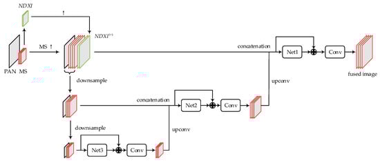
Figure 1.
The framework of the multi-scale deep residual network (MSDRN).
The network flowchart is for 4-band MS image, and the size ratio of PAN image to MS image is 4. In Figure 1, “↑” means upsampling operation. Moreover, it can be seen from Figure 1 that the entire network is divided into three levels, i.e., fine-level network, medium-level network and coarse-level network, from top to bottom. The networks in all levels have a similar structure, which consists of a sub-network (“Net” in the Figure) and a subsequent convolutional layer. The original data of the pansharpening problem is composed of MS image and PAN image, while that of the image deblurring network [35] is only one RGB image. To this end, the original MS image is first interpolated to the same size as the PAN image, and it is then stacked with the PAN image to form a 5-band data, which can be expressed as . Subsequently, the whole data is downsampled twice in succession, and the results are used as the initial inputs of the medium-level network and the coarse-level network, respectively. Each level of network outputs high-resolution MS image at the corresponding level.
Each level of the network is added a “skip connection”, which points from the input of the sub-network at each level to the output of the sub-network. Apart from stacking more layers, skip connections can also transmit the network’s input to the output intactly. In each level of the network, the network inputs including MS and PAN images of corresponding scale are transmitted unchanged to the output of the corresponding sub-network (Net), so that the loss of spectral information and spatial information in the fused image can be reduced. Since the element-wise addition operation requires the objects to be added to have the same dimensions, a convolutional layer needs to be added behind the skip connection to reduce the number of bands of the output data. Besides the initial inputs, the fused image from the next relatively coarser level is taken as part of the inputs by the medium- and fine-level networks. Specifically, the medium-level network uses the coarse-level fused image as part of inputs, and the fine-level network uses the fused image of the medium-level network as part of inputs. In this way, different levels of detail information from the source images can be exploited. In [26], the authors indicate that some class-specific radiometric indices having a high correlation to some feature maps from different layers can guide the learning process of the network. Hence, some well-known indices for 4-band MS, i.e., normalized difference water index (NDWI) and normalized difference vegetation index (NDVI) [26,38], are used in our proposed network. Their definitions can be expressed as
where represents corresponding band of MS. The concatenation of these extended inputs is expressed as NDXI, i.e., . In order to reduce the complexity of the network, they are only considered as part of the inputs of the fine-level network, because the fusion target of pansharpening is only generated by the fine-level network. Like the original MS image, NDXI is first interpolated to the same size as the PAN image, and these extended inputs of interpolating times are denoted as . Then, it is concatenated with the initial inputs (upsampled MS image and PAN image) of the fine-level network and fed into the fine-level network. The network fusion process is divided into three stages, starting with coarse-level fusion, transitioning to medium-level fusion, and ending at the final fine-level fusion. Here, the number of layers in each level of the network is set to l. The detailed descriptions of fusion are as follows.
Stage 1: The five-band data obtained by performing 4 × 4 downsampling is input to the coarse-level network. The output after the skip connection should also be five-band data, and it can be expressed as
where represents the mapping of “Net3” sub-network input to output; and represent the weights and biases of the sub-network, respectively; represents the th layer, and subscript “3” represents the coarse-level network. To obtain four-band coarse-level HRMS image, it is necessary to add another convolutional layer to reduce the spectral dimension, thus the resulting coarse-level HRMS image can be expressed as
where and , respectively, represent the weights and biases in the th layer of the coarse-level network, and represents the convolution operation.
Stage 2: To match the input image size of the medium-level network, the coarse-level fused image needs to be upsampled. The commonly used upsampling methods include the linear interpolation, bicubic interpolation, etc., but the up-convolution method is used in this paper. On the one hand, the up-convolution method has been claimed by some literatures [31,39] to have better performance. On the other hand, it can be used as a part of the entire network to make all layers of the entire network learn together without other interventions. The image after the coarse-level fused image is upsampled by a scale of 2 with the up-convolution method, which is denoted as . The coarse-level fused image after up-convolution is concatenated with the initial inputs of the medium-level network to form inputs with nine bands, which can be expressed as . Then, it is feed into the medium-level network, the output after the skip connection can be expressed as
where represents the mapping of “Net2” sub-network input to output; and , respectively, represent the weights and biases of the sub-network, and subscript “2” represents the medium-level network. Similarly, a convolutional layer needs to be added behind the skip connection, so that a medium-level HRMS image can be obtained by the following formula
where and respectively represent the weights and biases in the th layer of the medium-level network.
Stage 3: The medium-level HRMS image is upsampled by a scale of 2 with up-convolution manner, and the obtained image is expressed as . Concatenating the obtained image with the initial inputs of the fine-level network, the data obtained is used as the inputs of the fine-level network, and this whole data can be expressed as
Similar to the above two stages, the output after the skip connection of fine-level network and the output after adding the convolutional layer can be respectively expressed as
where is the final pansharpened image; , and represent the mapping of “Net1” sub-network input to output, the weights and biases of the sub-network; and , respectively, represent the weights and biases in the th layer of the fine-level network, and subscript “1” represents the fine-level network.
Except the up-convolution layers, each level of the network has the similar structure but different parameters, and number of layers is set to 11. The detailed structural parameters of the network are listed in Table 1.

Table 1.
Structural parameters of the MSDRN.
3.3. Training of Network
The goal of pansharpening is to obtain a HRMS image with the same spatial resolution as the PAN image, so it is desired that the spatial resolution of the fused image be as close as possible to that of the PAN image. However, the ideal image does not exist, which hampers the training of the network and the quality evaluation of the fused image. These problems can be solved by the Wald protocol [40]. The Wald protocol is to first downsample the original MS and PAN images at the same time based on the ratio of the spatial resolution of the MS and PAN images. The downsampled PAN image has the same spatial resolution as the original MS image. In this case, the original MS image can be used as a reference, and the downsampled MS and PAN images can be used as the inputs of the network. After the network training is completed, the original MS and PAN images are used as the inputs of the network, and the optimized model parameters are used to predict the pansharpened image.
The proposed network has three different levels of input and output. To make the network fully trained, a reference image is set at each level of the network. According to the Wald protocol, the reference images from the fine-level network to the coarse-level network respectively are the original MS image, the MS image after downsampling at the scale of 2, and the MS image after downsampling at the scale of 4. For the loss function, the mean square error (MSE) is chosen. In the case of reduced resolution, if the inputs of the fine-level to coarse-level network are simplified as , and , and the corresponding reference images are , and , respectively, then the loss function of the th level network can be expressed as
where 1, 2, 3, and i represents the number of the sample in a batch size; and represent the weights and biases of the th level network, respectively; denotes the mapping of th level network, and is the training batch size. During training, the loss functions of three different levels of network are averaged, i.e., the total loss function is
The optimal values of the parameters (weights and biases) are obtained by minimizing . The Adam [41] method is used to update the network parameters. If all the parameters in the network are expressed as , the update formula can be expressed as
where represents gradients at timestep ; and represent biased first moment estimate and biased second raw moment estimate, respectively; and represent bias-corrected first moment estimate and bias-corrected second raw moment estimate, respectively; represents the learning rate; , , are usually taken as , 0.99, 0.999, respectively.
4. Experiments
4.1. Datasets and Settings
The proposed MSDRN was tested on two different datasets, i.e., GeoEye-1 and Quickbird. As a commercial satellite of the United States, GeoEye-1 was launched in 2008, and it is one of the most advanced optical digital remote sensing satellites in the world today. The GeoEye-1 satellite carries a panchromatic sensor and a multispectral sensor. The former acquires a single-band panchromatic (PAN) image with a spatial resolution of 0.5 m, and the latter acquires a multispectral image with a spatial resolution of 2 m. The MS image has four bands, including red, green, blue, and near-infrared (Nir). The Quickbird satellite was launched by Digital Earth in 2001. It carries sensors that can acquire MS images with a spatial resolution of 0.6 m and PAN images with a resolution of 2.4 m. The bands of MS images obtained by Quickbird are the same as that of GeoEye-1. The main characteristics of the two satellites are shown in Table 2.
Table 2.
Spectral bands and spatial resolution of GeoEye-1 and Quickbird satellites.
Considering that different satellites have different characteristics, the model are trained and tested on two datasets, respectively. Each dataset is divided into two subsets, i.e., training set and test set, and the samples in these two subsets do not overlap. The group number of image patches of the training set and the test set are shown in Table 3. For each training set, the image patches are divided into three different levels, corresponding to the levels of the proposed network. From fine-level to coarse-level, the sizes of the training patches are 32 × 32, 16 × 16, and 8 × 8, respectively, where the latter two are obtained through downsampling the previous one by scales of 2 and 4, respectively. For each test set, a group of data is composed of an original 256 × 256 MS image and an original 1024 × 1024 PAN image. For the interpolation method, the polynomial interpolator with 23 coefficients proposed in the literature [42] are chosen.
Table 3.
Dataset division.
The deep learning framework PyTorch [43] is used to build the network, and the training process is supported by an Intel Core i7-10700 CPU. The training runs for 20 epochs maximumly. The initial learning rate is set to 0.001, and it decays by 50% every two epochs. The mini-batch size is set to 28. The training on each dataset takes about 20 h.
4.2. Quality Indicators
The simulated experiments use downsampled MS and PAN as the images to be fused and the original MS as a reference. The quality of the fused image is evaluated through six commonly used full-reference indicators, including spectral angle mapping (SAM) [44], erreur relative globale adimensionnelle de synthèse (ERGAS) [45], root mean square error (RMSE), correlation coefficient (CC), universal image quality index (Q) [46] and an extended version of Q () [47]. For experiments with real data, since there is no reference image, the quality no-reference index (QNR) [48], spectral distortion index and spatial distortion index are used. In the following description, the reference image and the fused image are denoted as and , respectively.
- SAM measures the spectral similarity between the pansharpened image and the corresponding reference image. A smaller value of SAM indicates a higher spectral similarity between two images. SAM is defined by the following formula
- ERGAS represents the degree of spatial distortion between the fused image and the reference image. The smaller the ERGAS, the higher the quality of the fused image. ERGAS is defined aswhere is the ratio of the spatial resolution between PAN and MS; is the number of MS bands; is the root mean square error between the band of the fused image and the reference image, and is the average of the original MS image band .
- RMSE measures the difference between pixel values of the fused image and the reference image. The smaller the RMSE, the closer the fused image to the reference image. RMSE is defined aswhere , and respectively represent the height, width, and band number of the MS image.
- CC reflects the strength of the correlation between the fused image and the reference image. The closer the CC is to 1, the stronger the correlation between the two objects. CC can be calculated by the following formulawhere represents the covariance between and , and represents the variance.
- Q can be used to estimate the global quality of the fused image. It measures the degree of correlation, the similarity of average brightness, and the similarity of contrast between the fused image and the reference image. The closer the value of Q is to 1, the better the quality of the fused image. The definition of Q iswhere represents the standard deviation of the image; represents the mean value of the image; represents the covariance between and .
- is an extended version of Q. It is also called Q4 when applied to four-band MS image, and Q8 when applied to eight-band MS image. It is defined aswhere and represent two quaternions (for four-band MS images) or two octonions (for eight-band MS images), which are respectively composed of radiation values of given image pixels in each band of reference MS image and fused MS image. introduces the measurement of spectral distortion of fused image based on Q. The closer the value is to 1, the better the fused image quality is.
- is an indicator that measures the spectral similarity between the fused image and the low-resolution MS image. The closer the value of is to 0, the more similar the spectral information between the fused image and the low-resolution MS image is. is defined byIn this formula, represents the fused image; represents the low-resolution MS image; Q represents the Q index; is the number of bands of the MS image; is a constant, and it is usually set to 1.
- is a measure of the spatial similarity between the fused image and the PAN image. The closer the value of is to 0, the smaller the spatial distortion of the fused image. is defined byIn the formula, refers to the PAN image and refers to the degraded PAN image; is a constant, and it is usually set to 1.
- QNR can measure both the spectral distortion and spatial distortion of the fused image, which is based on the spectral distortion index and the spatial distortion index . QNR is defined aswhere and control the relative degree of correlation between the spectral index and the spatial index. If and equal to 0 at the same time, QNR obtains the optimal value of 1.
4.3. Comparison Algorithms
To verify the effectiveness and reliability of the proposed network, some representative traditional algorithms and algorithms based on deep learning are selected for performance comparison. The selected traditional algorithms include the CS-based methods, such as IHS [2], PCA [4], BDSD [8], and PRACS [7]. The recently proposed robust BDSD (RBDSD) algorithm [49] is also considered, which is an extension of BDSD. As for the MRA-based methods, smoothing filter-based intensity modulation (SFIM) [50], ATWT with injection model 3 (ATWT_M3) [51], Indusion [52] and generalized Laplacian pyramid with MTF-matched filter (MTF_GLP) [53] are considered. Moreover, the AWLP with haze correction (AWLP_H) algorithm [54] is taken into consideration, which is an improved version of AWLP [14]. For the deep learning method, the PNN network [26] which first uses CNN for pansharpening and the deep residual network DRPNN proposed by Wei et al. [29] are selected. Most of the traditional algorithms are implemented based on the pansharpening toolbox provided by Vivone et al. [1].
4.4. The Influences of Scale Levels and Kernel Sizes
In this subsection, some experiments were conducted to discuss and analyze the influences of scale levels and kernel sizes on the performance of the proposed method. Firstly, we discuss and analyze the effect of the number of levels of the network on the performance of the proposed method. The experiments on , , and are conducted, respectively. The network with is shown in Figure 1. When , the coarse-level network is removed on the basis of the network shown in Figure 1; when , the bottom coarse-level network and the medium-level network are removed. As for the removal of the network, the inputs of the network are changed, while the unremoved network structure remains unchanged. In this set of comparative experiments, the convolution kernel sizes of the entire network are set to 3, and the remaining parameters are set as that described in Section 4.1. The simulated experiments were conducted on GeoEye-1 and QuickBird datasets, respectively. For each group of test images in two datasets, experiments were performed at different network levels, and the quality indicators of fused image were calculated. The curves showing the quality indicators of the fused image on two datasets with the image number are shown in Figure 2 and Figure 3, respectively.
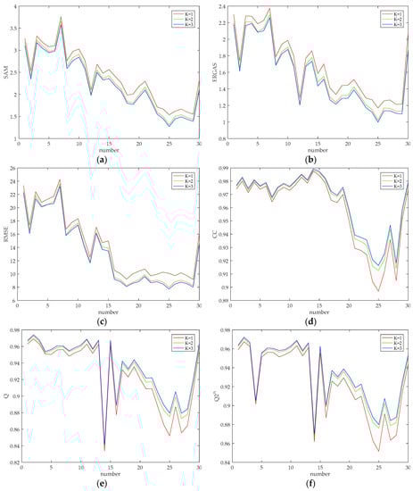
Figure 2.
Quality indicator curves of the fused image with network level set to 1, 2, and 3 on the GeoEye-1 dataset. (a) SAM; (b) ERGAS; (c) RMSE; (d) CC; (e) Q; (f) .
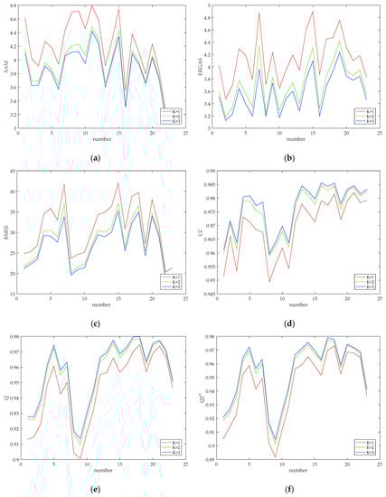
Figure 3.
Quality indicator curves of the fused image with network level set to 1, 2, and 3 on the QuickBird dataset. (a) SAM; (b) ERGAS; (c) RMSE; (d) CC; (e) Q; (f) .
From Figure 2 and Figure 3, it can be seen that as the network level increases, the six quality indicators all show better values, confirming the effectiveness of introducing multi-scale convolutional neural network into the pansharpening problem. However, increasing levels of the network results in a more complex network structure with more parameters needed to be trained; thus, the training time is increased, and an overfitting problem may be caused in the network. Therefore, to balance the relationship between the network performance and training time, the network level is finally set to 3.
After determining the level of the network, the kernel size of the convolutional layer is discussed, and its impact on the fusion result is explored. The kernel size of the up-convolutional layer is fixed to 3. In the experiments, the size of three convolution kernels is set, and two of them are set to the same value throughout the entire network, i.e., 3 and 5. In another case, considering that the patch size of input images in different levels of the network is different. Moreover, we assume that a smaller kernel is more suitable for extracting features of a smaller image patch, and a larger kernel tends to extract features of a larger image patch. Therefore, the kernel sizes from fine-level to coarse-level networks are set to 7, 5 and 3, respectively. The simulated experiments were conducted on all the test images of two datasets, and the curves showing the quality indicators of the fused images versus the image number are shown in Figure 4 and Figure 5, respectively. It can be seen from two figures that relatively better indicator values appear when the convolution kernel sizes are set to 3, and relatively poor indicator values appear when the convolution kernel is set to a larger size, although it is generally believed that a larger convolution kernel corresponds to a larger receptive field and can extract richer image information. However, this is not the case in our work, which may be due to the particularity of the pansharpening task. Therefore, the kernel sizes of the convolutional layer of the entire network are set to 3. A smaller convolution kernel indicates that fewer parameters need to be trained, which contributes to a decreased training time. Besides, it is worth mentioning that for the QuickBird dataset, setting the convolution kernel sizes of the fine-level network to the coarse-level network to 7, 5 and 3 is better than setting the convolution kernel sizes of the entire network to 5, which is different from the case appears in the GeoEye-1 dataset. This may be due to the different characteristics of different satellites.
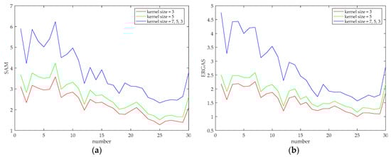
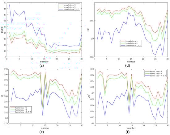
Figure 4.
Quality Indicator curves of different convolution kernel sizes (evaluated on 30 groups of test images of GeoEye-1 dataset). (a) SAM; (b) ERGAS; (c) RMSE; (d) CC; (e) Q; (f) .
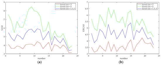
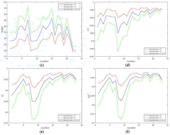
Figure 5.
Quality Indicator curves of different convolution kernel sizes (evaluated on 23 groups of test images of QuickBird dataset). (a) SAM; (b) ERGAS; (c) RMSE; (d) CC; (e) Q; (f) .
Based on the above discussion, it is determined that the number of levels of the proposed network is 3, and all the convolution kernel sizes of the entire network are also set to 3, as listed in Table 1.
4.5. Simulated Experiments
In this subsection, the simulated experiments were conducted on two datasets, and the proposed method is compared with some widely used algorithms (mentioned in Section 4.3). It should be illustrated that the optimal convolution kernel sizes of the original DRPNN [29] are 7. The DRPNN trained on our datasets with this setting, but relatively poor results were obtained during the performance test. Experiments have shown that better results are achieved when the convolution kernel sizes are set to 3 on our datasets, so the convolution kernel sizes of the DRPNN are set to 3 when comparing. Figure 6 and Figure 7, respectively, report the fusion results of our proposed MSDRN and other 12 algorithms on two datasets. Based on the results, it can be seen that compared with the upsampled low-resolution MS images using bicubic interpolation, the spatial resolution of the fused images obtained by all methods has been improved to a certain extent. For the CS-based methods, the algorithms including IHS, PCA and BDSD achieve high spatial resolution on two datasets. However, compared with the reference image (Ground Truth), these algorithms all suffer from spectral distortions, which is particularly evident for the IHS algorithm in Figure 7a. The RBDSD method produces some blurring effects in the fused images as shown in Figure 6d and Figure 7d. The fused images of the PRACS methods are shown in Figure 6e and Figure 7e; they show natural colors but some blurring effects in spatial details. As shown in Figure 6f,i, and Figure 7f,i, the SFIM and Indusion methods perform better on the QuickBird dataset but produce some spectral distortions on the GeoEye-1 dataset. It can be clearly observed from Figure 6g and Figure 7g that the AWLP_H method achieves good performance in both spatial resolution and spectral resolution. The ATWT_M3 method suffers from severe blurring and artifacts, especially on the white building near the middle of Figure 6h. The blurring also appears in the fused images of the MTF_GLP method with a relatively low degree as shown in Figure 6j and Figure 7j. Compared with the CS-based and MRA-based methods, the CNN-based methods show better performance in terms of spectral fidelity and spatial detail preservation, and the results obtained by them are very close to the reference images. In terms of the colors of the red buildings in the fused image of Figure 6, our proposed method and DRPNN perform better than PNN, showing the powerful potential of the deep network.
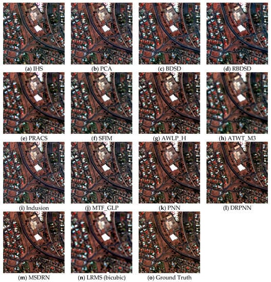
Figure 6.
An example of simulated experiments on the GeoEye-1 dataset. From (a–o) IHS, PCA, BDSD, RBDSD, PRACS, SFIM, AWLP_H, ATWT_M3, Indusion, MTF_GLP, PNN, DRPNN, MSDRN, LRMS (bicubic), Ground Truth.
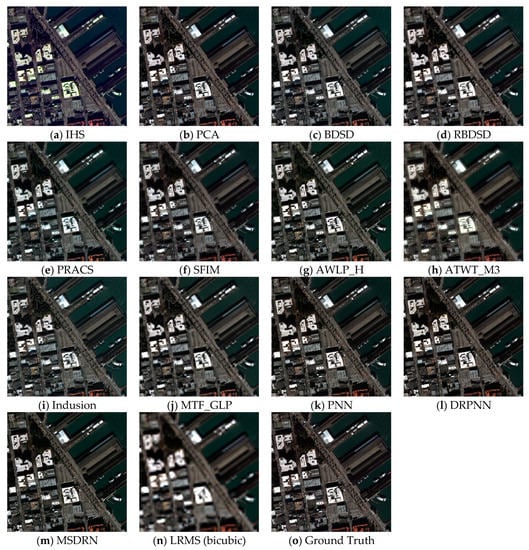
Figure 7.
An example of simulated experiments on the QuickBird dataset. From (a–o) IHS, PCA, BDSD, RBDSD, PRACS, SFIM, AWLP_H, ATWT_M3, Indusion, MTF_GLP, PNN, DRPNN, MSDRN, LRMS (bicubic), Ground Truth.
In addition to the subjective evaluation, the quantitative analysis of the fusion results is also essential. Table 4 and Table 5 report the quantitative assessment results of all methods on the GeoEye-1 and QuickBird datasets. The numerical values are obtained by averaging the evaluation results of the test images on the entire dataset. From Table 4 and Table 5, it can be seen that among the traditional CS-based algorithms, the BDSD and PRACS algorithms achieve the best results for the GeoEye-1 and the QuickBird datasets, respectively. As to the MRA-based algorithms, the SFIM and AWLP_H methods perform better. Among all the traditional algorithms, BDSD, SFIM, AWLP_H and PRACS achieve competitive and promising numerical values. Besides, it can be seen that our proposed MSDRN achieves the best results in all indicators, indicating that MSDRN can effectively improve the spatial detail quality of the fused images while reducing spectral distortion. In addition, the other two methods based on deep learning, PNN and DRPNN, achieving satisfactory results. Furthermore, the deep learning methods surpass the traditional algorithms in terms of all indicator values, fully demonstrating the powerful potential and performance of deep learning technology to solve the pansharpening problem.
Table 4.
Quantitative evaluation comparison of fusion results on the GeoEye-1 dataset.
Table 5.
Quantitative evaluation comparison of fusion results on the QuickBird dataset.
4.6. Real Data Experiments
The original MS and PAN images need to be fused in practical applications. In the experiments on real data, the original MS and PAN images are taken as inputs, and the model parameters used in the simulated experiments are also used to generate a fused image. Examples of fused images on two datasets are shown in Figure 8 and Figure 9. In these two figures, a rectangle region is magnified and put at the bottom of each image.
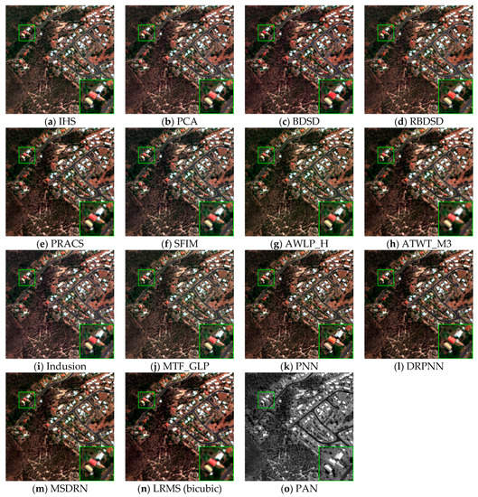
Figure 8.
An example of real data experiments conducted on the GeoEye-1 dataset. From (a–o) IHS, PCA, BDSD, RBDSD, PRACS, SFIM, AWLP_H, ATWT_M3, Indusion, MTF_GLP, PNN, DRPNN, MSDRN, LRMS (bicubic), PAN.
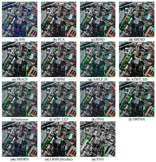
Figure 9.
An example of real data experiments conducted on the QuickBird dataset. From (a–o) IHS, PCA, BDSD, RBDSD, PRACS, SFIM, AWLP_H, ATWT_M3, Indusion, MTF_GLP, PNN, DRPNN, MSDRN, LRMS (bicubic), PAN.
Through the observation and comparison illustrated in Figure 8, the results obtained by most fusion methods are greatly improved compared with the LRMS images using bicubic interpolation and show the similar phenomena as in the simulated experiments. It can be seen that the ATWT_M3 method produces obvious spatial blurring. The IHS method suffers from serious spectral distortion. In addition, BDSD and PNN also suffer from some spectral distortions. It can be observed from the magnified regions that the former appears on the red buildings with deeper color in the fused image, which is called over-saturation; the latter appears on the red buildings with lighter color. The result obtained by the Indusion method exhibits serious artifacts, and this phenomenon is also shown in the result obtained by MTF_GLP. The DRPNN method produces slight spectral distortion. For our proposed method, both the spatial information and the spectral information are preserved to produce relatively better results.
In Figure 9, it can be observed that some methods exhibit similar phenomena that appear in Figure 8, such as IHS, ATWT_M3, BDSD, Indusion, MTF_GLP, etc. In addition, it can be seen that the PNN method also results in some artifacts in the magnified region, and the PRACS method produces a slight spatial blurring. In contrast, the other pansharpening algorithms obtain relatively better fusion results. The fused image of our method is shown in Figure 9m, which shows good spatial and spectral qualities. It demonstrates that the proposed MSDRN method achieves competitive performance.
Since there is no reference image, no-reference indicators are used to evaluate the performances of various fusion methods, i.e., , and QNR. Table 6 lists the quantitative evaluation results of two datasets, in which the numerical values are obtained by averaging the indictor values of all the test images. From the results, it can be seen that the PNN achieves good results for most indicators on the GeoEye-1 dataset. Besides, the BDSD and PRACS also achieve impressive performances, showing the superior numerical values among traditional algorithms. In general, the top values of most indicators are obtained by the deep learning methods, indicating the great potential and good performances of the methods based on deep learning. Our proposed method achieves the best QNR and values on the QuickBird dataset but produces slight spectral and spatial distortion on the GeoEye-1 dataset. However, compared with most traditional algorithms, our algorithm still has some advantages.
Table 6.
Quantitative evaluation comparison of real data experiments on two datasets.
5. Conclusions
Deep learning technology has made remarkable achievements in many fields, fully demonstrating the great potential and considerable performance of this technology. In this paper, a MSDRN pansharpening method is proposed. Based on the original three-layer network in SRCNN and PNN, the strategy of coarse-to-fine is explored to make full use of the details of different scales of the original images. Experimental results demonstrate that the progressive reconstruction scheme is beneficial to improve the quality of the fused image. Moreover, residual learning is used to extract deeper-level features of the images and simplify the learning process. Experimental results on the GeoEye-1 and QuickBird datasets demonstrate that when the scale level is fixed as 3 and the kernel size is fixed as 3, the proposed method achieves the best performance. The fused images produced by the proposed method exhibit better spectral and spatial qualities compared with those of 12 pansharpening methods. For two types of simulated data, the proposed method provides the best SAM, ERGAS, RMSE, CC, Q, and values. For the real data, the proposed method still has better values in terms of QNR, , and . In general, the proposed method has superior fusion performance for different remote sensing images.
In the future work, more feasible solutions that can further improve the network performance will be studied, and a solution that combines deep learning methods with traditional methods will be considered. In addition, hyperspectral and panchromatic/multispectral image fusion is an interesting issue. Actually, the pansharpening is a special instance of hyperspectral and panchromatic/multispectral image fusion. Our future work will also study improving the proposed method and applying it to hyperspectral and panchromatic/multispectral image fusion.
Author Contributions
Conceptualization, W.W., Z.Z., H.L. and G.X.; methodology, W.W. and Z.Z.; software, Z.Z.; validation, W.W.; investigation, Z.Z.; resources, W.W.; writing—original draft preparation, Z.Z.; writing—review and editing, W.W., Z.Z., H.L. and G.X.; visualization, Z.Z.; supervision, H.L. and G.X.; funding acquisition, W.W., H.L. and G.X. All authors have read and agreed to the published version of the manuscript.
Funding
This work was supported in part by the National Natural Science Foundation of China under Grants 61703334,61973248,61873201, by the Project funded by China Postdoctoral Science Foundation under Grant 2016M602942XB, and by Key Projection of Shaanxi Key Research and Development Program under Grant 2018ZDXM-GY-089.
Institutional Review Board Statement
Not applicable.
Informed Consent Statement
Not applicable.
Data Availability Statement
Data sharing is not applicable to this article.
Conflicts of Interest
The authors declare no conflict of interest.
References
- Vivone, G.; Alparone, L.; Chanussot, J.; Dalla Mura, M.; Garzelli, A.; Licciardi, G.A.; Restaino, R.; Wald, L. A critical comparison among pansharpenig algorithms. IEEE Trans. Geosci. Remote Sens. 2015, 53, 2565–2586. [Google Scholar] [CrossRef]
- Tu, T.M.; Su, S.C.; Shyu, H.C.; Huang, P.S. A new look at IHS-like image fusion methods. Inf. Fusion. 2001, 2, 177–186. [Google Scholar] [CrossRef]
- Tu, T.M.; Huang, P.S.; Hung, C.L.; Chang, C.P. A fast intensity hue-saturation fusion technique with spectral adjustment for IKONOS imagery. IEEE Geosci. Remote Sens. Lett. 2004, 1, 309–312. [Google Scholar] [CrossRef]
- Shahdoosti, H.R.; Ghassemian, H. Combining the spectral PCA and spatial PCA fusion methods by an optimal filter. Inf. Fusion. 2016, 27, 150–160. [Google Scholar] [CrossRef]
- Laben, C.; Brower, B. Process for Enhancing the Spatial Resolution of Multispectral Imagery Using Pan-Sharpening. U.S. Patent 6,011,875, 4 January 2000. [Google Scholar]
- Gillespie, A.; Kahle, A.B.; Walker, R.E. Color enhancement of highly correlated images-II. Channel ration and “Chromaticity” Transform techniques. Remote Sens. Environ. 1987, 22, 343–365. [Google Scholar] [CrossRef]
- Choi, J.; Yu, K.; Kim, Y. A new adaptive component-substitution-based satellite image fusion by using partial replacement. IEEE Trans. Geosci. Remote Sens. 2011, 49, 295–309. [Google Scholar] [CrossRef]
- Garzelli, A.; Nencini, F.; Capobianco, L. Optimal MMSE pansharpening of very high resolution multispectral images. IEEE Trans. Geosci. Remote Sens. 2008, 46, 228–236. [Google Scholar] [CrossRef]
- Vivone, G.; Restaino, R.; Mura, M.D.; Licciardi, G.; Chanussot, J. Contrast and Error-Based Fusion Schemes for Multispectral Image Pansharpening. IEEE Geosci. Remote Sens. Lett. 2014, 11, 930–934. [Google Scholar] [CrossRef]
- Shensa, M.J. The discrete wavelet transform: Wedding the à trous and Mallat algorithm. IEEE Trans. Signal Process. 1992, 40, 2464–2482. [Google Scholar] [CrossRef]
- Nencini, F.; Garzelli, A.; Baronti, S.; Alparone, L. Remote sensing image fusion using the curvelet transform. Inf. Fusion 2007, 8, 143–156. [Google Scholar] [CrossRef]
- Aiazzi, B.; Alparone, L.; Baronti, S.; Garzelli, A.; Selva, M. An MTF-based spectral distortion minimizing model for pan-sharpening of very high resolution multispectral images of urban areas. In Proceedings of the 2nd GRSS/ISPRS Joint Workshop on Remote Sensing and Data Fusion over Urban Areas, Berlin, Germany, 22–23 May 2003. [Google Scholar] [CrossRef]
- Chavez, P.S., Jr.; Sides, S.C.; Anderson, A. Comparison of three different methods to merge multiresolution and multispectral data: Landsat TM and SPOT panchromatic. Photogramm. Eng. Remote Sens. 1991, 57, 295–303. [Google Scholar] [CrossRef]
- Otazu, X.; González-Audìcana, M.; Fors, O.; Nùñez, J. Introduction of sensor spectral response into image fusion methods. Application to wavelet-based methods. IEEE Trans. Geosci. Remote Sens. 2005, 43, 2376–2385. [Google Scholar] [CrossRef]
- Zhong, S.W.; Zhang, Y.; Chen, Y.S.; Wu, D. Combining component substitution and multiresolution analysis: A novel generalized BDSD pansharpening algorithm. IEEE J. Sel. Top. Appl. Earth Obs. Remote Sens. 2017, 10, 2867–2875. [Google Scholar] [CrossRef]
- Li, S.; Yang, B. A new pansharpening method using a compressed sensing technique. IEEE Trans. Geosci. Remote Sens. 2011, 49, 738–746. [Google Scholar] [CrossRef]
- Li, S.; Yin, H.; Fang, L. Remote Sensing Image Fusion via Sparse Representations Over Learned Dictionaries. IEEE Trans. Geosci. Remote Sens. 2013, 51, 4779–4789. [Google Scholar] [CrossRef]
- Ayas, S.; Gormus, E.T.; Ekinci, M. An Efficient PanSharpening via Texture Based Dictionary Learning and Sparse Representation. IEEE J. Sel. Topics Appl. Earth Obs. Remote Sens. 2018, 7, 2448–2460. [Google Scholar] [CrossRef]
- Zhu, X.X.; Bamler, R. A sparse image fusion algorithm with application to pansharpening. IEEE Trans. Geosci. Remote Sens. 2013, 51, 2827–2836. [Google Scholar] [CrossRef]
- Fei, R.; Zhang, J.; Liu, J.; Du, F.; Chang, P.; Hu, J. Convolutional Sparse Representation of Injected Details for Pansharpening. IEEE Goesci. Remote Sens. Lett. 2019, 16, 1595–1599. [Google Scholar] [CrossRef]
- Yin, H. Sparse representation based pansharpening with details injection model. Signal Process. 2015, 113, 218–227. [Google Scholar] [CrossRef]
- Dong, C.; Loy, C.; He, K.; Tang, X. Image super-resolution using deep convolutional networks. IEEE Trans. Pattern Anal. Mach. Intell. 2016, 38, 295–307. [Google Scholar] [CrossRef]
- Zhang, K.; Zuo, W.; Chen, Y.; Meng, D.; Zhang, L. Beyond a Gaussian denoiser: Residual learning of deep CNN for image denoising. IEEE Trans. Image Process. 2017, 26, 3142–3155. [Google Scholar] [CrossRef] [PubMed]
- Svoboda, P.; Hradis, M.; Marŝík, L.; Zemcík, P. CNN for license plate motion deblurring. In Proceedings of the 2016 IEEE International Conference on Image Processing (ICIP), Phoenix, AZ, USA, 25–28 September 2016. [Google Scholar] [CrossRef]
- Zhang, P.; Gong, M.; Su, L.; Liu, J.; Li, Z. Change detection based on deep feature representation and mapping transformation for multi-spatial resolution remote sensing images. ISPRS J. Photogramm. Remote Sens. 2016, 116, 24–41. [Google Scholar] [CrossRef]
- Masi, G.; Cozzolino, D.; Verdoliva, L.; Scarpa, G. Pansharpening by convolutional neural networks. Remote Sens. 2016, 8, 594. [Google Scholar] [CrossRef]
- Scarpa, G.; Vitale, S.; Cozzolino, D. Target-Adaptive CNN-Based Pansharpening. IEEE Trans. Geosci. Remote Sens. 2018, 56, 5443–5457. [Google Scholar] [CrossRef]
- He, K.; Zhang, X.; Ren, S.; Sun, J. Deep residual learning for image recognition. In Proceedings of the 2016 IEEE Conference on Computer Vision and Pattern Recognition (CVPR), Las Vegas, NV, USA, 27–30 June 2016. [Google Scholar] [CrossRef]
- Wei, Y.; Yuan, Q.; Shen, H.; Zhang, L. Boosting the Accuracy of Multispectral Image Pansharpening by Learning a Deep Residual Network. IEEE Geosci. Remote Sens. Lett. 2017, 14, 1795–1799. [Google Scholar] [CrossRef]
- Yuan, Q.; Wei, Y.; Meng, X.; Shen, H.; Zhang, L. A Multiscale and Multidepth Convolutional Neural Network for Remote Sensing Imagery Pan-Sharpening. IEEE J. Sel. Top. Appl. Earth Obs. Remote Sens. 2018, 3, 978–989. [Google Scholar] [CrossRef]
- Liu, X.; Liu, Q.; Wang, Y. Remote sensing image fusion based on two-stream fusion network. Inf. Fusion. 2020, 55, 1–15. [Google Scholar] [CrossRef]
- Zhong, J.; Yang, B.; Huang, G.; Zhong, F.; Chen, Z. Remote sensing image fusion with convolutional neural network. Sens. Imaging 2016, 17, 1–16. [Google Scholar] [CrossRef]
- Wang, D.; Li, Y.; Ma, L.; Bai, Z.; Chan, J.C.W. Going Deeper with Densely Connected Convolutional Neural Networks for Multispectral Pansharpening. Remote Sens. 2019, 11, 2608. [Google Scholar] [CrossRef]
- Yang, Y.; Tu, W.; Huang, S.; Lu, H. PCDRN: Progressive Cascade Deep Residual Network for Pansharpening. Remote Sens. 2020, 12, 676. [Google Scholar] [CrossRef]
- Nah, S.; Kim, T.H.; Lee, K.M. Deep Multi-scale Convolutional Neural Network for Dynamic Scene Deblurring. In Proceedings of the 2017 IEEE Conference on Computer Vision and Pattern Recognition (CVPR), Honolulu, HI, USA, 21–26 July 2017. [Google Scholar] [CrossRef]
- Denton, E.L.; Chintala, S.; Fergus, R. Deep generative image models using a laplacian pyramid of adversarial networks. In Proceedings of the 28th International Conference on Neural Information Processing Systems, Palais des Congrès de Montréal, Montréal, QC, Canada, 7–12 December 2015. [Google Scholar]
- Eigen, D.; Puhrsch, C.; Fergus, R. Depth map prediction from a single image using a multi-scale deep network. In Proceedings of the 27th International Conference on Neural Information Processing Systems, Montréal, QC, Canada, 8–13 December 2014. [Google Scholar]
- Pan, H.; Li, X.; Wang, W.; Qi, C. Mariculture Zones Extraction Using NDWI and NDVI. Adv. Mater. Res. 2013, 659, 153–155. [Google Scholar] [CrossRef]
- Long, J.; Shelhamer, E.; Darrell, T. Fully convolutional networks for semantic segmentation. IEEE Trans. Pattern Anal. Mach. Intell. 2017, 39, 640–657. [Google Scholar] [CrossRef]
- Wald, L.; Ranchin, T.; Mangolini, M. Fusion of satellite images of different spatial resolution:Assessing the quality of resulting images. Photogramm. Eng. Remote Sens. 1997, 63, 691–699. [Google Scholar] [CrossRef]
- Kingma, D.; Ba, J.L. Adam: A method for stochastic optimization. In Proceedings of the 3rd International Conference for Learning Representations (ICLR), San Diego, CA, USA, 7–9 May 2015. [Google Scholar]
- Aiazzi, B.; Alparone, L.; Baronti, S.; Garzelli, A. Context-driven fusion of high spatial and spectral resolution images based on oversampled multiresolution analysis. IEEE Trans. Geosci. Remote Sens. 2002, 40, 2300–2312. [Google Scholar] [CrossRef]
- PyTorch. Available online: https://pytorch.org (accessed on 12 December 2020).
- Yuhas, R.H.; Goetz, A.F.H.; Boardman, J.W. Discrimination among semi-arid landscape endmembers using the Spectral AngleMapper (SAM) algorithm. In Summaries of the Third Annual JPL Airborne Geoscience Workshop; AVIRIS Workshop: Pasadena, CA, USA, 1992; pp. 147–149. [Google Scholar]
- Wald, L. Data Fusion: Definitions and Architectures-Fusion of Images of Different Spatial Resolutions; Presses des Mines: Paris, France, 2002. [Google Scholar]
- Wang, Z.; Bovik, A. A universal image quality index. IEEE Signal Process. Lett. 2002, 9, 81–84. [Google Scholar] [CrossRef]
- Garzelli, A.; Nencini, F. Hypercomplex quality assessment of multi/hyper-spectral images. IEEE Geosci. Remote Sens. Lett. 2009, 6, 662–665. [Google Scholar] [CrossRef]
- Alparone, L.; Aiazzi, B.; Baronti, S.; Garzelli, A.; Nencini, F.; Selva, M. Multispectral and panchromatic data fusion assessment without reference. Photogramm. Eng. Remote Sens. 2008, 74, 193–200. [Google Scholar] [CrossRef]
- Vivone, G. Robust Band-Dependent Spatial-Detail Approaches for Panchromatic Sharpening. IEEE Trans. Geosci. Remote Sens. 2019, 57, 6421–6433. [Google Scholar] [CrossRef]
- Liu, J. Smoothing filter-based intensity modulation: A spectral preserve image fusion technique for improving spatial details. Int. J. Remote Sens. 2000, 21, 3461–3472. [Google Scholar] [CrossRef]
- Ranchin, T.; Wald, L. Fusion of high spatial and spectral resolution images: The ARSIS concept and its implementation. Photogramm. Eng. Remote Sens. 2000, 66, 49–61. [Google Scholar] [CrossRef]
- Khan, M.M.; Chanussot, J.; Condat, L.; Montavert, A. Indusion: Fusion of multispectral and panchromatic images using the induction scaling technique. IEEE Trans. Geosci. Remote Sens. 2008, 5, 98–102. [Google Scholar] [CrossRef]
- Aiazzi, B.; Alparone, L.; Baronti, S.; Garzelli, A.; Selva, M. MTF tailored multiscale fusion of high-resolution MS and pan imagery. Photogramm. Eng. Remote Sens. 2006, 72, 591–596. [Google Scholar] [CrossRef]
- Vivone, G.; Alparone, L.; Garzelli, A.; Lolli, S. Fast reproducible pansharpening based on instrument and acquisition modeling: AWLP Revisited. Remote Sens. 2019, 11, 2315. [Google Scholar] [CrossRef]


Publisher’s Note: MDPI stays neutral with regard to jurisdictional claims in published maps and institutional affiliations. |
© 2021 by the authors. Licensee MDPI, Basel, Switzerland. This article is an open access article distributed under the terms and conditions of the Creative Commons Attribution (CC BY) license (http://creativecommons.org/licenses/by/4.0/).