Article

Global Assessment of the GNSS Single Point Positioning Biases Produced by the Residual Tropospheric Delay

1
College of Surveying and Geo-informatics, Tongji University, 1239 Siping Road, Shanghai 200092, China
2
State Key Laboratory of Information Engineering in Surveying, Mapping and Remote Sensing, Wuhan University, 129 Luoyu Road, Wuhan 430079, China
*
Author to whom correspondence should be addressed.
Remote Sens. 2021, 13(6), 1202; https://doi.org/10.3390/rs13061202
Submission received: 31 January 2021 / Revised: 13 March 2021 / Accepted: 16 March 2021 / Published: 22 March 2021
(This article belongs to the Special Issue Advances in GNSS Data Processing and Navigation)

Abstract

:
The tropospheric delay is one of the main error sources that degrades the accuracy of Global Navigation Satellite Systems (GNSS) Single Point Positioning (SPP). Although an empirical model is usually applied for correction and thereby to improve the positioning accuracy, the residual tropospheric delay is still drowned in measurement noise, and cannot be further compensated by parameter estimation. How much this type of residual error would sway the SPP positioning solutions on a global scale are still unclear. In this paper, the biases on SPP solutions introduced by the residual tropospheric delay when using nine conventionally Zenith Tropospheric Delay (ZTD) models are analyzed and discussed, including Saastamoinen+norm/Global Pressure and Temperature (GPT)/GPT2/GPT2w/GPT3, University of New Brunswick (UNB)3/UNB3m, European Geostationary Navigation Overlay System (EGNOS) and Vienna Mapping Functions (VMF)3 models. The accuracies of the nine ZTD models, as well as the SPP biases caused by the residual ZTD (dZTD) after model correction are evaluated using International GNSS Service (IGS)-ZTD products from around 400 globally distributed monitoring stations. The seasonal, latitudinal, and altitudinal discrepancies are analyzed respectively. The results show that the SPP solution biases caused by the dZTD mainly occur on the vertical direction, nearly to decimeter level, and significant discrepancies are observed among different models at different geographical locations. This study provides references for the refinement and applications of the nine ZTD models for SPP users.

Graphical Abstract

1. Introduction

Due to the high operational efficiency and algorithm simplicity, pseudorange-based Single Point Positioning (SPP) is still the most popular Global Navigation Satellite Systems (GNSS) positioning technology for custom-grade navigation where meter-level positioning accuracy is sufficient [1]. Compared with Precise Point Positioning (PPP) and Network Real Time Kinematic (NRTK), SPP does not restricted to convergence time and reference stations. One of the major error sources that degrades the SPP accuracy is the signal transmission delay caused by the troposphere [2]. The so-called tropospheric delay varies from about 2 m at the zenith to 20 m at lower elevation angles between receiver and satellite [3]. Typically, an empirical model is applied to mitigate the tropospheric delay and therewith to improve the positioning accuracy [4,5]. Usually, the residual tropospheric delay after model correction will be further estimated in PPP and NRTK applications, so as to mitigate the biases projecting to positioning. However, in SPP, the residual tropospheric delay is drowned in measurement noise, and cannot be further compensated by parameter estimation. Therefore, it is necessary to assess the biases produced by the residual tropospheric delay on SPP.
Usually the tropospheric delay along the line-of-sight is mapped onto the zenith direction using the elevation-dependent mapping function [6]. Therefore, modeling the Zenith Tropospheric Delay (ZTD) is essential. Up till now, a variety of tropospheric delay models have been proposed and discussed. They are mainly divided into two classes: (1) the models relying on meteorological parameters as inputs, such as Hopfield model [7] and Saastamoinen model [8]; and (2) the models based on a look-up table to provide meteorological parameters, such as University of New Brunswick (UNB) series models and the European Geostationary Navigation Overlay System (EGNOS) model [9,10]. Funded by the Austrian Science Fund, TU Wien provides abundant tropospheric products as open access data [11]. The released discrete troposphere delay models (e.g., VMF1 and VMF3) are based on actual data from Numerical Weather Models (NWMs) by the European Center for Medium-Range Weather Forecasts (ECMWF) [12], and are provided either in grid-wise or site-wise. Furthermore, other hybrid ZTD models, such as GZTD2 [13], IGGtrop_ri (i = 1, 2, and 3) [14], TropGrid2 [15], Improved Tropospheric Grid (ITG) [16], the improved wet delay model [17], IGGtrop_SH and IGGtrop_rH [18], WGTEM [19], and so on, have been successively developed, with the purpose of improving accuracy and simplifying calculation.
ZTD is conventionally expressed as the sum of the Zenith Hydrostatic Delay (ZHD) and the Zenith Wet Delay (ZWD) [20]. Due to the high temporal and spatial variability of atmospheric water vapor, it is difficult to model the ZWD precisely [21], which accordingly limits the correction accuracies of different ZTD methods. Many investigations have been focusing on evaluating the correction accuracies of these models. Tuka and El-Mowafy [22] compared several tropospheric models with the Saastamoinen model at six IGS stations and concluded that the models used in their study showed higher accuracies at mid-latitude regions than at the equator. Yao et al. [16] concluded that the Saastamoinen+GPT2 model is 10% better than the UNB3m model, referring to the IGS-ZTD products. By using 1-year data from 27 IGS monitoring stations, Liu et al. [23] concluded that the Saastamoinen+GPT2w model is superior to the Saastamoinen+GPT2 model. Zhang et al. [24] evaluated the accuracy of IGGtrop, EGNOS, and UNB3m models in China using 25 stations of the Crustal Movement Observation Network of China. The results show that the accuracy of IGGtrop is about 24% and 19% higher than that of EGNOS and UNB3m models, respectively. Yao et al. [25] assessed the consistence between VMF-ZTD forecast grid products and IGS-ZTD products, and concluded that the difference is at the centimeter level. Yuan et al. [26] assessed the forecast Vienna Mapping Function 1 for real-time tropospheric delay modeling in GNSS, and concluded that the model performs of the VMF1-FC are better than GPT2 and GPT2w. Li et al. [27] conducted a comprehensively accuracy analysis on nine ZTD models (UNB3m, EGNOS, Saastamoinen+GPT2/GPT2w/GPT3, Hopfield+GPT2/GPT2w/GPT3, and IGGtropSH models) at 65 Antarctic stations. The results showed that the Saastamoinen+GPT2/GPT2w/GPT3 models are better than the other six models.
It is unquestioned that newer, more elegant models generally have higher accuracy than those older and more complicated one. For example, the VMF models, with centimeter discrepancies to IGS ZTD products, have already been recognized as a standard for precise positioning users [26]. Although this kind of grid-wise model can be easily applied at anytime and anywhere via interpolation, requisition for frequent updates still restricts its application for real-time positioning, in which empirical models, such as the Saastamoinen and UNB series models, are still preferred due to higher operational efficiency. In these cases, the uncorrected residual zenith tropospheric delay would still sway the GNSS SPP solution remarkably. However, how much the uncorrected residual tropospheric delay would sway the GNSS positioning solution on a global scale are still unclear. In this paper, with the purpose of evaluating the biases caused by the uncorrected residual tropospheric delay on SPP solutions globally, nine conventionally used ZTD models are analyzed and discussed, including Saastamoinen+norm/GPT/GPT2/GPT2w/GPT3, UNB3, UNB3m, EGNOS, and VMF3 model. Firstly, the residual ZTDs were obtained by comparing the model estimation values with the corresponding IGS ZTD products at 400 IGS monitoring stations, to evaluate the accuracies of the ZTD models. The spatial and temporal variations of the residual ZTDs by different models are here discussed. Then the biases on SPP solutions introduced by the residual ZTDs were computed, and the temporal and spatial characteristics were analyzed.
This paper is organized as follows. The calculation procedure for the influence of residual tropospheric delay on SPP are described in Section 2. Then, the materials, methodology and the data processing strategy used for the assessment are introduced in Section 3. Next, the results of the residual ZTDs obtained from different models and their impacts on SPP solution are presented in Section 4. The results are briefly discussed in Section 5 and the conclusions are summarized in Section 6.

2. Influences of Residual Tropospheric Delays on Single Point Positioning

Generally, the GNSS pseudo-range and carrier phase are generally expressed as [28]
{ P r , f s = ρ r , f s + t r t s + α r s T z + β f I r s + b r , f s + ε P Φ r , f s = ρ r , f s + t r t s + α r s T z β f I r s + d r , f s λ f N r , f s + ε Φ
in which, P r , f s , Φ r , f s are pseudo-range and carrier phase from receiver r to satellite s (s = 1, …, j) on frequency f( f = 1, …, k) in length units, respectively; ρ is the geometric distance,; tr and ts are the receiver and satellite clock error in length units, respectively; Tz is the ZTD that can be converted to slant with the mapping function α; I denotes the line-of-sight (LOS) total electron content (TEC) with the frequency dependent factor βf = 40.3/f2; b r , f s and d r , f s are frequency-receiver-satellite dependent signal delays related to pseudo-range and carrier phase observables; N is the integer ambiguity.
For single-epoch single-station point positioning, only pseudo-range observables are applied. Without specifying the frequency, the linearized observation model for positioning is [29]
l = A x + e   and   var ( e ) = D e e
where l = P ρ 0 is the observation residual vector, A = ( u   I ) is design matrix with u being the LOS unit vector from the user to satellite; e is the random error vector with covariance D e e . The unknown parameters in conventional SPP model usually contains four elements, as x = [ δ x δ y δ z t r ] T , with δ x , δ y and δ z are three coordinate component corrections and t r is the receiver clock error.
In SPP, the tropospheric delays are usually corrected by empirical models, and ionospheric delays are mitigated either by empirical models or by inter-frequency difference. In this paper, we mainly concentrate on the impacts of residual tropospheric delays on the SPP solutions after model correction. Therefore, the observation residual vectors in Equation (2) are specified as
{ l 0 = P ρ 0 α T Z 0 l 1 = P ρ 0 α T Z
where T Z 0 and T Z are the model estimated and unknown true value of the station ZTD in meters, respectively; α is the elevation-related mapping coefficient vector. According to least-squares estimation principle, the corresponding unknown parameters are estimated as [29]
{ x ^ i = D x ^ i x ^ i A T D e e 1 l i var ( x ^ i ) = D x ^ i x ^ i = ( A T D e e 1 A ) 1                   i = 0 , 1
And the residual error vector of the observables are estimated as [29]
{ e ^ i = R l i R = I A D x ^ i x ^ i A T D e e 1 var ( e ^ i ) = D e ^ i e ^ i = D e e A D x ^ i x ^ i A T                   i = 0 , 1
According to Equations (4) and (5), it is concluded that the residual ZTDs only cause biases on the estimated parameters, and do not influence the estimated covariances. Therefore, corresponding biases on the estimated unknown parameters can be given as
δ x ^ = x ^ 1 x ^ 0 = D x ^ i x ^ i A T D e e 1 α · d Z T D
where d Z T D = ( T Z T Z 0 ) is the residual ZTD after model correction. Equation (6) indicates that the residual ZTD will be projected to the SPP solution with a mapping coefficient vector m = D x ^ i x ^ i A T D e e 1 α . With a prior variance model D e e , m is determined by the station geographical location and observing time epoch. Therefore, the SPP solution biases δ x ^ can be estimated at anytime and anywhere once residual ZTD (dZTD) is obtained.

3. Materials and Methods

In this section, the most commonly used ZTD models and products are summarized, and the data processing strategies are presented.

3.1. ZTD Model

There are two main types of ZTD models, combined and empirical models. The combined model estimates the ZTD via a combination of a meteorological model and a classic ZTD model which requires meteorological parameters, while the empirical model obtains the required meteorological parameters from a look-up table that usually depends on station latitude and height, as well as observation time.

3.1.1. Combined Model

The classic ZTD model requires in-site meteorological data, which is usually calculated by the meteorological model. The most popular classic ZTD model is the Saastamoienen model.
In the Saastamoienen model, the troposphere is divided into two layers. The first layer is from the earth surface to 10 km height of the troposphere, where the temperature descent rate is 6.5 °C/km. The second layer is from the troposphere top at 10 km to the stratospheric top at 70 km, where the temperature is assumed to be constant. Via atmospheric refraction integral, the function is simplified as [8]
{ Z T D = 0.002277 × [ P + ( 0.05 + 1255 T + 273.15 ) e ] f ( φ , H ) f ( φ , H ) = 1 2.66 × 10 3 c o s ( 2 φ ) 2.8 × 10 7 H
where P, T, and e are the pressure, temperature, and water vapor pressure at the station, f(φ, H) is the correction of gravitational acceleration caused by the rotation of the Earth, with φ and H denoting the latitude and the ortho height of the station, respectively.
In-site meteorological elements used in Equation (7) can be estimated via a set of meteorological models, such as the norm, GPT/GPT2/GPT2w/GPT3 models.
The standard meteorological element method (norm) is based on a set of standard meteorological parameters on sea level (usually specified as T0 = 288.15 K, P0 = 1013.25 mbar, e0 = 11.691 mbar), and adjusted to the station via a height correction.
The Global Pressure and Temperature (GPT) model [30], which is based on spherical harmonics up to degree and order nine, provides pressure (P) and temperature (T) at any site on the Earth’s surface. It is based on the atmospheric pressure and temperature products (resolution 15° × 15°) in the meteorological reanalysis data ECMWF Re-Analysis-40 (ERA-40) for 3 years from 1999 to 2002, and conforms to changes in air pressure and temperature on the global sea level.
To precisely describe the spatial and temporal variability, GPT2 model [31] based on 10-year meteorological reanalysis data ERA-Interim were established. The model provides pressure (P), temperature (T), lapse rate (dT), water vapor pressure (e), and mapping function coefficients at any site, resting upon a global 5° grid of mean values, annual, and semi-annual variations in all parameters.
Global Pressure and Temperature 2 wet (GPT2w) [32] is the successor of the former models GPT and GPT2, improving the capability to determine ZWDs empirically. It requires only information about time and location and provides mean values plus annual and semi-annual amplitudes of a set of quantities such as mapping function coefficients, pressure (P), temperature (T), water vapor pressure (e), mean temperature weighted with water vapor pressure (Tm), and water vapor decrease factor (λ), optionally on a 5° × 5° or a 1° × 1° grid. The coefficients were derived from monthly mean pressure-level data of ERA-Interim fields by the ECMWF. Landskron and Böhm [11] proposed a new GPT3 model, which provides the same meteorological elements as those in GPT2w. The several meteorological quantities from GPT2w are left unchanged for GPT3. In addition, the ray-traced delays are also utilized for determining an empirical gradient grid which outperforms currently existing models. Finally, primary information of the above five meteorological models are summarized in Table 1 for a detailed comparison.

3.1.2. Empirical Model

Collins et al. [33] proposed the UNB3 model for the Wide Area Augmentation System (WAAS) users. The UNB3 model depends on a look-up table to calculate the five meteorological parameters; namely, pressure (P), temperature (T), water vapor pressure (e), temperature lapse rate ( β ), and water vapor pressure height factor ( λ ) on the station. These meteorological parameters are estimated by inputting the receiver’s height, latitude, and day of year (DOY), and are interpolated from the yearly averages and seasonal variations of the parameters that are primarily derived from North American meteorological data. These meteorological parameters are then used to compute the hydrostatic and non-hydrostatic zenith delays using a model which is similar as the Saastamoninen models.
UNB3m [9] is a modified version of the UNB3, with changes on parameter values in the look-up table and the associated UNB3 algorithms. The part of the table that was related to water vapor pressure was replaced with values that computed from the relative humidity. Hydrostatic delay will not be affected by this modification in the model, since it does not depend on the water vapor pressure. By ray-tracing analyses of 703,711 profiles from 223 stations in North America and surrounding territory from 1990 to 1996, it is evaluated that the prediction errors of UNB3m is similar to that of UNB3, and the absolute mean error has been reduced by almost 75%.
The European Geo-stationary Navigation Overlay System (EGNOS) guidelines recommend that a user applies a correction for tropospheric delay that is compliant with the International Civil Aviation Organization (ICAO) Standards and Recommended Practices (SARPs) for Satellite-Based Augmentation Systems (SBAS). The recommended SBAS model, termed simply the EGNOS model, utilizes the same look-up table as UNB3 to provide empirical meteorological parameters, and then calculates the ZTD by simplified equations where the Earth Gravity parameter is assumed to be constant [10].
Finally, Table 2 summarizes the major information of the above three empirical models, where similarities and differences among them are listed.

3.2. Products

Apart from correction models, more accurate ZTD products have been provided by TU Wien and the International GNSS Service (IGS), named as VMF-ZTD and IGS-ZTD. Primary information about the two are introduced in this subsection, with a brief summarization in Table 3.

3.2.1. VMF-ZTD

TU Wien provides ZTD products as a part of the proposed Vienna Mapping Functions (VMF) which can be found at the webpage: https://vmf.geo.tuwien.ac.at/ accessed on 9 August 2020.
The discrete VMF are based on direct raytracing through NWM by using meteorological data from the ECMWF [34]. Currently, two versions are available for the user, namely VMF1 and VMF3.
The VMF1 [35] is a model providing discrete values for ZHD, ZWD and the hydrostatic and wet mapping functions “mfh” and “mfw”. It relies on empirical equations for the “b” and “c” coefficients of the continued fraction form, whereas the “a” coefficients are determined from rigorously ray-traced mapping functions at 3° elevation based on the information of NWMs by the ECMWF. VMF1 are provided on a global grid (2.5° × 2.0°) as well as at IGS sites, and the time resolution is 6 h.
VMF3 is the successor of VMF1, with refined model accuracy. Ray-traced delays for 10 years of ECMWF ERA-Interim re-analysis data on a global grid was used to re-determine empirical mapping function coefficients ”b” and “c” through spherical harmonics expansions up to degree and order 12, by which spatial as well as temporal components are equipped [12]. The grid-wise VMF3 data is available in a horizontal resolution of 5° × 5° as well as 1°× 1°, and in a time resolution of 6 h.

3.2.2. IGS-ZTD

The International GNSS Service (IGS) has been providing the total ZTD products for global monitoring stations since 1997. Between 1997 and 2003, a weighted average combined product was generated by independent products from multiple analysis centers. The product adopts the SINEX format, with a time resolution of 2 h and an accuracy of about 4 mm [36]. Since 2003, a new ZTD product was acquired by the Jet Propulsion Laboratory (JPL) Analysis Center using GIPSY software with Precise Point Positioning (PPP) procedure and Neil Mapping Function (NMF). A 5-minute-resolution ZTD file was provided with an official accuracy of 1.5–5 mm. Due to the systematic error, the actual error is slightly larger [37]. Since 2011, The United States Naval Observatory (USNO) assumed responsibility for producing IGS final ZTD products by Bernese GNSS Software 5.2 [38]. The processing used PPP and the Global Mapping Function (GMF) with IGS final satellite orbits/clocks and earth orientation parameters as input, and the elevation angle cutoff is 7 degrees [39,40].

3.3. Data Processing Strategy

To evaluate the accuracies of abovementioned nine models, IGS ZTD products from 372 to 404 globally distributed monitoring stations were used as references, by which accuracies of nine conventionally used ZTD models or products are evaluated, including saas+norm/GPT/GPT2/GPT2w/GPT3, UNB3, UNB3m, EGNOS and VMF3. In order to analyze the seasonal discrepancies, the data from four 7-day periods in 2019 were selected during spring, summer, autumn, and winter periods. The data time slots were DOY 80–86, DOY 172–178, DOY 266–272, and DOY 356–362 respectively. The corresponding day of year (DOY) and the number of available stations (num) are shown in the Table 4. Figure 1 shows the distribution of global IGS GPS stations. The sampling rate IGS-ZTD produces is 5 min, therefore the model values were computed at every 5 min. For VMF3, the cubic spline interpolation method was used to interpolate the 6 h products to 5 min. Since the Saastamoinen model requires meteorological parameters as inputs, the first step was to calculate the meteorological data by the norm/GPT/GPT2/GPT2w/GPT3 model, and then the ZTD values were calculated by the Saastamoinen model. The GPT model does not provide the water vapor, therefore the same value as that in the norm model was used. Regarding the IGS-ZTD as the “true value”, and the residual ZTD (dZTD) of each model can be calculated as
d Z T D = Z T D I G S t Z T D M t
where Z T D I G S t and Z T D M t are the IGS-ZTD and model-calculated ZTD at the time epoch t, respectively. Mean and Root Mean Square (RMS) values of the dZTD were used to measure the bias and stability of the ZTD models, respectively.
mean = 1 N i = 1 N ( d Z T D i )
RMS = 1 N i = 1 N ( d Z T D i ) 2
where N is the total number of observations.
As derived in Section 2, the biases on SPP caused by the dZTD were further calculated by substituting dZTD into Equation (6). The GPS satellite constellation was used, and the elevation cut-off angle was 7 degrees, which is consistent with IGS-ZTD. The GMF [41] and IGS final satellite orbits were used for the calculation.

4. Result

In this section, the characteristics of the residual zenith tropospheric delay (dZTD) of nine ZTD models and their impacts on the SPP solution are presented.

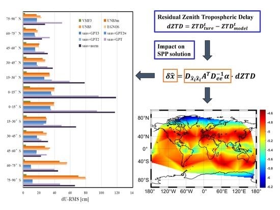
4.1. The Residual Zenith Tropospheric Delay (dZTD)

Firstly, the mean and RMS values of the dZTD by the nine models were calculated via data from all stations and in all days, as shown in Figure 2. It shows that among these models, the dZTD mean and RMS values by saas+norm/GPT were significantly larger than those by other models. The reason for this is that the meteorological parameters used in the saas+norm/GPT are quite rough and have low accuracy. Comparably, saas+GPT2/GPT2w/GPT3 show much better performances. The dZTD means and RMSs by these three models are all less than 1 cm and 5 cm, respectively. The performances of EGNOS/UNB3/UNB3m were also comparative, and were all slightly worse than the saas+GPT2/GPT2w/GPT3. The biases by EGNOS/UNB3 were less than 2 cm, while that of UNB3m was significantly reduced to 0.35 cm. This is because the UNB3m model uses relative humidity instead of water vapor pressure in the look-up table, which improves the calculation accuracy of the ZWD. However, dZTD RMSs of the three models were similar, all around 6 cm. Also, it is interesting to note that biases by combined models (saas+) were positive, and biases by empirical models (EGNOS/UNB3/UNB3m) were negative. As a more accurate product, the bias of VMF3-ZTD is ignorable, and the RMS is just 1.31 cm. Therefore, it can be concluded that IGS-ZTD and VMF3-ZTD products are on similar accuracy level.
From Figure 3 we can see that dZTD means by most models show obvious discrepancies in different seasons. For the saas+norm model, the dZTD mean value in summer is the largest (around 9 cm), and those in spring and winter were much smaller (around 5 cm). The seasonal discrepancy of the saas+GPT model was most significant, with biases mainly existing in summer and autumn, and nearly ignorable in spring and winter. Biases of saas+GPT2/GPT2w/GPT3 models were remarkably reduced, and were also slightly larger in summer. Comparably, biases of saas+GPT2 were always smaller than the other two in different seasons. In terms of the three empirical models, the biases of EGNOS and UNB3m were similar, and both larger than those of UNB3m models. It is noted that the biases of EGNOS and UNB3 models in summer were much smaller than those in other three seasons, and biases of UNB3m were most significant in winter and almost ignorable in other three seasons. At last, the biases of VMF3-ZTD were comparable in the four seasons, and always close to 0.
Figure 4 show the dZTD RMSs of different models by season. Generally, RMSs in summer are always the largest, and RMSs in the other three seasons are comparable for all these nine models. These nine models can be divided into four groups, that are saas+norm/GPT, EGNOS/UNB3/UNB3m, saas+GPT2/GPT2w/GPT3, and VMF3. The model stabilities are comparable within each group, and significantly increase among groups. Specifically, RMSs of EGNOS/UNB3/UNB3m are nearly 30% smaller than saas+GPT, and are 20% larger than saas+GPT2/GPT2w/GPT3. RMSs of VMF3 are the smallest, which are improved by about 70% compared to the GPT2/GPT2w/GPT3 model.
The results above show that the correction accuracies of different ZTD models could be remarkably different, and the model accuracies are usually lower in summer. Generally, newer, more elegant models have higher accuracy than those older and more complicated one. However, operational burdens for the former are also heavier. As shown in Figure 5, the average run time of eight models (saas+norm/GPT/GPT2/GPT2w/GPT3, EGNOS, UNB3, UNB3m) was counted by using MATLAB software. It counted data from 400 stations with a time slot of 28 days, and the data sampling rate was 5 min. It showed that the computation efficiency of the Saastamoinen model is 100 times higher than saas+GPT/GPT2/GPT2w/GPT3, and 30 times higher than EGNOS/UNB/UNB3 models. For real-time practical applications, users should make balance between higher accuracy and higher computation efficiency. Empirical models, such as Saastamoinen, are still popular when the requirement for positioning accuracy is not so stringent, but higher computation efficiency is necessary.
In the next subsection, biases on SPP solutions produced by the uncorrected residual ZTD when adopting different ZTD models are evaluated globally and the spatiotemporal characteristics are analyzed. With these results, custom-grade SPP users are capable of anticipating the positioning deviation from the unknown real location when using different tropospheric delay correction models.

4.2. The Impacts of the Residual Zenith Tropospheric Delay on the SPP Solution

In this subsection, impacts of the dZTD on the SPP solution are analyzed. Table 5 shows the means and RMSs of the SPP biases on North (N), East (E), and Up (U) direction produced by the dZTD of the nine models. One can see that the biases mainly occur on the U direction, nearly to decimeter level. In contrast, biases on the horizontal (N and E) direction are significantly smaller, just at the centimeter level. Among all these models, the SPP biases by using the saas+norm model are the largest, with means being 0.16 cm, 0.04 cm, −35.6 cm, and RMSs being 4.08 cm, 3.31 cm, 44.55 cm on the N, E, U directions respectively. The SPP biases of using the EGNOS/UNB3/UNB3m models are slightly larger and less stable than those of saas+GPT2/GPT2w/GPT3 models. It is noted that SPP biases on the vertical direction are negative when using saas+ models, and those values are positive when using EGNOS/UNB3/UNB3m models. At last, the SPP biases by using the VMF3 model are the smallest, with means being −0.01 cm, 0 cm, 0.79 cm, and RMSs being 0.59 cm, 0.43 cm, 5.93 cm on N, E, U directions respectively. In general, the dZTD impacts on SPP solutions are negligible on horizontal directions and significant on vertical direction. Therefore, only the SPP solution impacts on the vertical direction are further analyzed below.
To evaluate the SPP solutions influenced by the uncorrected ZTD when using different models in different seasons, the RMSs of the SPP biases on the vertical direction produced by dZTD of the nine models are shown in Figure 6 by season. Compared with Figure 4, one can see that similar tendencies on the SPP solutions are observed. The RMSs in summer are generally the largest, and RMSs in spring and winter are equivalent and slightly smaller than those in autumn. One exception is the saas+GPT, where RMSs in spring and winter are much larger than those in summer and autumn. For VMF3, the seasonal discrepancies are less significant, even though the RMSs in summer are still slightly larger. In generally, it can be concluded that SPP solution stability would be relatively lower in summer regardless of the ZTD model.
To compare the model discrepancies in different geographical locations, the dZTD RMSs (upper panels) and RMSs of the SPP biases on the vertical direction (lower panels) generated by dZTD from saas+GPT (left panels) and UNB3 (right panels) models at globally distributed IGS stations are shown in Figure 7. Triangulation linear interpolation is used for the demonstration. One can see that the saas+GPT model performs worst around the equator, and best around middle latitude areas. Near the equator, the dZTD RMSs can exceed 20 cm and accordingly cause over 100 cm biases on the SPP solutions in the vertical direction. In contrast, more significant asymmetry between southern and northern hemispheres is observed by using the UNB3 model. The performance of UNB3 model is significantly better in the northern hemisphere, especially around middle and high latitudes (40°N~90°N), where the dZTD RMSs are below 5 cm and RMSs of SPP vertical biases are below 20 cm.
Equation (6) indicates that the residual ZTD will be projected to the SPP solution with a mapping coefficient vector m = D x ^ i x ^ i A T D e e 1 α . To further analyze the relationship between dZTD and the SPP biases on the vertical direction, the means of the mapping coefficient between dZTD and the SPP biases on the vertical direction at globally distributed IGS stations are shown in Figure 8. It can be seen that the mapping coefficient is negative and approximately symmetrical along the equator. The mean value reaches the minimum (around −4.6) at mid-latitude zones, and then increases to around −5.4 at equatorial, and around −6 at polar zones. This implies that the dZTD values would be adversely magnified about five times on the SPP vertical solutions globally, and the impacts are slightly smaller at mid-latitude zones.
In Figure 7 we can see that the SPP biases show significant discrepancies along different latitudes. Therefore, the globally distributed stations are divided into groups with a latitude interval of 15°, and RMS of the vertical SPP biases caused by dZTDs from the nine models were further calculated for each latitude region. The station numbers at different latitude regions are shown in Figure 9 and RMSs of the vertical SPP biases by using the nine models at different latitude regions are shown in Figure 10.
Figure 9 shows that nearly 50% of these stations are located on 30°N~60°N, and stations beyond 60°S~60°N are rare. Figure 10 shows that RMS of the vertical SPP biases caused by dZTDs from the nine models are significantly different at different latitudes, and tendencies among models are inconsistent. Around equatorial regions (30°S~30°N), the SPP biases for saas+norm/GPT models reach the largest (around 100 cm) which are 2–3 times as much as those for UNB3/UNB3m/EGNOS and saas+GPT2/GPT2w/GPT3. While the model discrepancies decrease relatively at middle latitude regions (30S°~60°S and 30N°~75°N), and RMSs of SPP biases by using these models are all reduced to below 40 cm. In the regions of 60S°~90°S, RMSs of SPP biases by using UNB3/UNB3m/EGNOS and saas+norm/GPT models gradually increase to 50 cm, and those by using saas+GPT2/GPT2w/GPT3 further reduced to around 10 cm. In the regions of 45N°~90°N, RMSs of SPP biases by using UNB3/UNB3m/EGNOS and saas+GPT2/GPT2w/GPT3 models are nearly stable, all less than 20 cm, while those for saas+norm/GPT models increase slightly to around 30 cm and 50 cm respectively. The VMF3 model performs well globally, with a relatively larger uncertainty around the equator, where the RMSs of SPP vertical biases are still less than 10 cm.
To further evaluate the SPP accuracies and stabilities influenced by different ZTD models at different altitudes, the globally distributed stations were divided into groups along to their station heights (orthometric height) and RMSs of the vertical SPP biases by using these models were calculated within each altitude region. Considering that ZTD has a large number of stations within 500 m, and the variation is large within 500 m [42], the group of station heights were subdivided into seven groups. The station numbers at different altitudes regions are shown in Table 6 and RMSs of the vertical SPP biases by using the nine models at different altitudes regions are shown in Figure 11.
Table 6 shows that nearly 75% of these stations are below 500 m and stations with height above 2000 m are rare. Figure 11 shows that RMSs of the vertical SPP biases by using the nine models generally show significant downward trends as the heights increase except for the saas+GPT2 and VMF3 models. The saas+GPT2 model performs best on stations with heights between 500~1000 m, and significantly worst on stations above 2000 m. The VMF3 performs equally at different height regions. The results coincide with the fact that ray tracing used for producing VMF3 products considers changes with height. In general, the vertical SPP solutions would suffer more significantly influence by the uncorrected ZTD at lower stations.

5. Discussion

By now, SPP is still the most popular mode for custom-grade positioning and navigation applications, in which the Saastamoienen model with standard meteorological parameter, the UNB-series models and the EGNOS model are prevailingly applied, other than those newer grid-wise models, e.g., the GPT and VMF series, since frequent data communication and higher operational burden are required by the latter. In contrast, the latter generally have higher accuracy than the former. Therefore, it is worth to anticipate how much the uncorrected residual ZTD would sway the SPP solution in different locations around the world, so that SPP users can optimally determine which ZTD model is used to seek the highest computation efficiency under required positioning precision. For reference, the following recommendations are provided:
(1) If users just request meter-level horizontal positioning accuracy and are not concerned with vertical positioning accuracy, the simplest Saastamoienen model is preferred.
(2) For users located at 30°S–90°S, the Saastamoienen model is a better choice compared with UNB3/UNB3m/EGNOS models.
(3) For users located near the equator areas, the Saastamoienen model is not an optimal choice, since the SPP biases caused by uncorrected residual ZTD would be at least three times as large as those caused by using other models.
(4) For users at Northern Hemisphere, UNB3m model would be optimal. Since it can achieve similar accuracy to the saas+GPT series models and the computation efficiency is significantly higher.
(5) If the vertical SPP biases produced by residual ZTD are required to be lower than 10 cm, only the VMF3 model can be used.
(6) It is anticipated that the SPP solution on vertical direction would be higher than the real value when using Saas+ models and would be lower than the real value when using UNB3/UNB3m/EGNOS models.

6. Conclusions

In this study, the accuracies of nine zenith tropospheric delay (ZTD) models, as well as the SPP biases caused by the residual ZTD (dZTD) after model correction were evaluated using IGS-ZTD products from around 400 globally distributed monitoring stations. The nine ZTD models are saas+norm/GPT/GPT2/GPT2w/GPT3, UNB3, UNB3m, EGNOS, and VMF3. The seasonal, latitudinal, and altitudinal discrepancies were analyzed respectively. From the study, the following conclusions can be obtained:
(1) The nine models can be generally divided into four groups, that are saas+norm/GPT, EGNOS/UNB3/UNB3m, saas+GPT2/GPT2w/GPT3, and VMF3. The model accuracies and stabilities are comparable within each group, and significantly increase among groups. RMSs of EGNOS/UNB3/UNB3m are nearly 30% smaller than saas+GPT, and are 20% larger than saas+GPT2/GPT2w/GPT3. The bias of VMF3-ZTD is ignorable, and the RMS is just 1.31 cm.
(2) The SPP solution biases caused by the dZTD mainly occur on the vertical (U) direction, nearly to decimeter level, and biases on horizontal (N and E) directions are significantly smaller, just at centimeter level. Generally, the dZTD values are adversely magnified about 5 times on the vertical SPP solution biases globally, and the impacts are slightly smaller at mid-latitude zones.
(3) In terms of seasonal effects, all of the nine models show lower stabilities in summer, and stabilities in the other three seasons are comparable. For latitude effects, the four groups show inconsistent tendencies. Generally, these models show larger variations and discrepancies at equatorial and south polar regions. Finally, for altitude effects, the model stabilities generally increase as the station heights increase except for the saas+GPT2 and VMF3 models.
By the above assessments and analyses, the question of how much the uncorrected dZTD would sway the SPP solution on a global scale is answered. Meanwhile, references for the refinement and applications of the nine ZTD models are provided.

Author Contributions

Conceptualization, L.Y.; methodology, L.Y. and J.W.; software, J.W.; validation, L.Y. and H.L.; formal analysis, L.Y. and J.W.; investigation, L.Y. and J.W.; resources, H.L. and T.B.; data curation, J.W.; writing—original draft preparation, J.W. and L.Y.; writing—review and editing, L.Y. and J.W.; visualization, H.L. and T.B.; supervision, H.L. and T.B.; project administration, H.L. and T.B.; funding acquisition, H.L. and T.B. All authors have read and agreed to the published version of the manuscript.

Funding

This research was funded by the National Natural Science Foundation of China (41504022), the Shanghai Natural Science Foundation (20ZR1462000), and the Open Research Fund Program of LIESMARS (Grant No. 19R02).

Data Availability Statement

Publicly available datasets were analyzed in this study. These data can be found here: [https://vmf.geo.tuwien.ac.at/ accessed on 9 August 2020] and [ftp://cddis.gsfc.nasa.gov/gps/data accessed on 20 January 2019].

Acknowledgments

The authors would like to thank IGS and TU Wien for providing zenith tropospheric delay products.

Conflicts of Interest

The authors declare no conflict of interest.

References

  1. Zheng, F.; Gu, S.; Gong, X.; Lou, Y.; Fan, L.; Shi, C. Real-Time Single-Frequency Pseudorange Positioning in China Based on Regional Satellite Clock and Ionospheric Models. GPS Solut. 2020, 24, 1–13. [Google Scholar] [CrossRef]
  2. Tregoning, P.; Herring, T.A. Impact of a Priori Zenith Hydrostatic Delay Errors on GPS Estimates of Station Heights and Zenith Total Delays. Geophys. Res. Lett. 2006, 33. [Google Scholar] [CrossRef] [Green Version]
  3. Janes, H.W.; Langley, R.B.; Newby, S.P. Analysis of Tropospheric Delay Prediction Models: Comparisons with Ray-Tracing and Implications for GPS Relative Positioning. Bull. Géodésique 1991, 65, 151–161. [Google Scholar] [CrossRef]
  4. Davis, J.L.; Herring, T.A.; Shapiro, I.I.; Rogers, A.E.E.; Elgered, G. Geodesy by Radio Interferometry: Effects of Atmospheric Modeling Errors on Estimates of Baseline Length. Radio Sci. 1985, 20, 1593–1607. [Google Scholar] [CrossRef]
  5. Jin, S.G.; Luo, O.; Ren, C. Effects of Physical Correlations on Long-Distance GPS Positioning and Zenith Tropospheric Delay Estimates. Adv. Space Res. 2010, 46, 190–195. [Google Scholar] [CrossRef]
  6. Kačmařík, M.; Douša, J.; Dick, G.; Zus, F.; Brenot, H.; Möller, G.; Pottiaux, E.; Kapłon, J.; Hordyniec, P.; Václavovic, P.; et al. Inter-Technique Validation of Tropospheric Slant Total Delays. Atmos. Meas. Tech. 2017, 10, 2183–2208. [Google Scholar] [CrossRef] [Green Version]
  7. Hopfield, H.S. Two-Quartic Tropospheric Refractivity Profile for Correcting Satellite Data. J. Geophys. Res. 1969, 74, 4487–4499. [Google Scholar] [CrossRef]
  8. Saastamoinen, J. Introduction to Practical Computation of Astronomical Refraction. Bull. Geod. 1972, 106, 383–397. [Google Scholar] [CrossRef]
  9. Leandro, R.F.; Langley, R.B.; Santos, M.C. UNB3m_pack: A Neutral Atmosphere Delay Package for Radiometric Space Techniques. GPS Solut. 2008, 12, 65–70. [Google Scholar] [CrossRef]
  10. Penna, N.; Dodson, A.; Chen, W. Assessment of EGNOS Tropospheric Correction Model. J. Navig. 2001, 54, 37–55. [Google Scholar] [CrossRef] [Green Version]
  11. Landskron, D.; Böhm, J. VMF3/GPT3: Refined Discrete and Empirical Troposphere Mapping Functions. J. Geod. 2018, 92, 349–360. [Google Scholar] [CrossRef] [PubMed]
  12. Hofmeister, A.; Böhm, J. Application of Ray-Traced Tropospheric Slant Delays to Geodetic VLBI Analysis. J. Geod. 2017, 91, 945–964. [Google Scholar] [CrossRef] [PubMed] [Green Version]
  13. Yao, Y.; Hu, Y.; Yu, C.; Zhang, B.; Guo, J. An Improved Global Zenith Tropospheric Delay Model GZTD2 Considering Diurnal Variations. Nonlin. Process. Geophys. 2016, 23, 127–136. [Google Scholar] [CrossRef] [Green Version]
  14. Li, W.; Yuan, Y.; Ou, J.; Chai, Y.; Li, Z.; Liou, Y.-A.; Wang, N. New Versions of the BDS/GNSS Zenith Tropospheric Delay Model IGGtrop. J. Geod. 2015, 89, 73–80. [Google Scholar] [CrossRef]
  15. Schüler, T. The TropGrid2 Standard Tropospheric Correction Model. GPS Solut. 2014, 18, 123–131. [Google Scholar] [CrossRef]
  16. Yao, Y.; Xu, C.; Shi, J.; Cao, N.; Zhang, B.; Yang, J. ITG: A New Global GNSS Tropospheric Correction Model. Sci. Rep. 2015, 5, 10273. [Google Scholar] [CrossRef] [Green Version]
  17. Dousa, J.; Elias, M. An Improved Model for Calculating Tropospheric Wet Delay. Geophys. Res. Lett. 2014, 41, 4389–4397. [Google Scholar] [CrossRef]
  18. Li, W.; Yuan, Y.; Ou, J.; He, Y. IGGtrop_SH and IGGtrop_rH: Two Improved Empirical Tropospheric Delay Models Based on Vertical Reduction Functions. IEEE Trans. Geosci. Remote Sens. 2018, 56, 5276–5288. [Google Scholar] [CrossRef]
  19. Xu, C.; Yao, Y.; Shi, J.; Zhang, Q.; Peng, W. Development of Global Tropospheric Empirical Correction Model with High Temporal Resolution. Remote Sens. 2020, 12, 721. [Google Scholar] [CrossRef] [Green Version]
  20. Hofmeister, A. Determination of Path Delays in the Atmosphere for Geodetic VLBI by Means of Ray-Tracing. Ph.D. Thesis, Technischen Universitat Wien Fakultat fur Mathematik und Geoinformation, Vienna, Austria, 2016. [Google Scholar]
  21. Meunram, P.; Satirapod, C. Spatial Variation of Precipitable Water Vapor Derived from GNSS CORS in Thailand. Geod. Geodyn. 2019, 10, 140–145. [Google Scholar] [CrossRef]
  22. Tuka, A.; El-Mowafy, A. Performance Evaluation of Different Troposphere Delay Models and Mapping Functions. Measurement 2013, 46, 928–937. [Google Scholar] [CrossRef] [Green Version]
  23. Liu, J.; Chen, X.; Sun, J.; Liu, Q. An Analysis of GPT2/GPT2w+Saastamoinen Models for Estimating Zenith Tropospheric Delay over Asian Area. Adv. Space Res. 2017, 59, 824–832. [Google Scholar] [CrossRef]
  24. Zhang, H.; Yuan, Y.; Li, W.; Li, Y.; Chai, Y. Assessment of Three Tropospheric Delay Models (IGGtrop, EGNOS and UNB3m) Based on Precise Point Positioning in the Chinese Region. Sensors 2016, 16, 122. [Google Scholar] [CrossRef] [Green Version]
  25. Yao, Y.; Xu, X.; Xu, C.; Peng, W.; Wan, Y. GGOS Tropospheric Delay Forecast Product Performance Evaluation and Its Application in Real-Time PPP. J. Atmos. Sol. Terr. Phys. 2018, 175, 1–17. [Google Scholar] [CrossRef]
  26. Yuan, Y.; Holden, L.; Kealy, A.; Choy, S.; Hordyniec, P. Assessment of Forecast Vienna Mapping Function 1 for Real-Time Tropospheric Delay Modeling in GNSS. J. Geod. 2019, 93, 1501–1514. [Google Scholar] [CrossRef]
  27. Li, F.; Zhang, Q.; Zhang, S.; Lei, J.; Li, W. Evaluation of Spatio-Temporal Characteristics of Different Zenith Tropospheric Delay Models in Antarctica. Radio Sci. 2020, 55, e2019RS006909. [Google Scholar] [CrossRef]
  28. Nie, Z.; Liu, F.; Gao, Y. Real-Time Precise Point Positioning with a Low-Cost Dual-Frequency GNSS Device. GPS Solut. 2020, 24, 1–11. [Google Scholar] [CrossRef]
  29. Xu, G.; Xu, Y. GPS Theory, Algorithms and Applications; Springer: Berlin/Heidelberg, Germany, 2016; ISBN 978-3-662-50365-2. [Google Scholar]
  30. Boehm, J.; Heinkelmann, R.; Schuh, H. Short Note: A Global Model of Pressure and Temperature for Geodetic Applications. J. Geod. 2007, 81, 679–683. [Google Scholar] [CrossRef]
  31. Lagler, K.; Schindelegger, M.; Böhm, J.; Krásná, H.; Nilsson, T. GPT2: Empirical Slant Delay Model for Radio Space Geodetic Techniques: GPT2: EMPIRICAL SLANT DELAY MODEL. Geophys. Res. Lett. 2013, 40, 1069–1073. [Google Scholar] [CrossRef] [PubMed] [Green Version]
  32. Böhm, J.; Möller, G.; Schindelegger, M.; Pain, G.; Weber, R. Development of an Improved Empirical Model for Slant Delays in the Troposphere (GPT2w). GPS Solut. 2015, 19, 433–441. [Google Scholar] [CrossRef] [Green Version]
  33. Collins, P.; Langley, R.; LaMance, J. Limiting Factors in Tropospheric Propagation Delay Error Modelling for GPS Airborne Navigation. In Proceedings of the institute of navigation 52nd annual meeting, Cambridge, MA, USA, 19–21 June 1996; p. 10. [Google Scholar]
  34. Boehm, J. Vienna Mapping Functions in VLBI Analyses. Geophys. Res. Lett. 2004, 31, L01603. [Google Scholar] [CrossRef]
  35. Kouba, J. Implementation and Testing of the Gridded Vienna Mapping Function 1 (VMF1). J. Geod. 2008, 82, 193–205. [Google Scholar] [CrossRef]
  36. Dow, J.M.; Neilan, R.E.; Rizos, C. The International GNSS Service in a Changing Landscape of Global Navigation Satellite Systems. J. Geod. 2009, 83, 191–198. [Google Scholar] [CrossRef]
  37. Byun, S.H.; Bar-Sever, Y.E. A New Type of Troposphere Zenith Path Delay Product of the International GNSS Service. J. Geod. 2009, 83, 1–7. [Google Scholar] [CrossRef] [Green Version]
  38. Dach, R.; Lutz, S.; Walser, P.; Fridez, P. (Eds.) Bernese GNSS Software Version 5.2; User Manual, Astronomical Institute; University of Bern, Bern Open Publishing: Bern, Switzerland, 2015; ISBN 978-3-906813-05-9. [Google Scholar] [CrossRef]
  39. Hackman, C.; Guerova, G.; Byram, S.; Dousa, J.; Hugentobler, U. International GNSS Service (IGS) troposphere products and working group activities. FIG Working Week. In Proceedings of the Wisdom of the Ages to the Challenges of the Modern World, Sofia, Bulgaria, 17–21 May 2015; pp. 1–14. [Google Scholar]
  40. Villiger, A.; Dach, R. (Eds.) International GNSS Service Technical Report 2018 (IGS Annual Report). IGS Cent. Bur. Univ. Bern 2019. [Google Scholar] [CrossRef]
  41. Boehm, J.; Niell, A.; Tregoning, P.; Schuh, H. Global Mapping Function (GMF): A New Empirical Mapping Function Based on Numerical Weather Model Data. Geophys. Res. Lett. 2006, 33, L07304. [Google Scholar] [CrossRef] [Green Version]
  42. Liangke, H.; Lilong, L.; Chaolong, Y. A Zenith Tropospheric Delay Correction Model Based on the Regional CORS Network. Geod. Geodyn. 2012, 3, 53–62. [Google Scholar] [CrossRef] [Green Version]
Figure 1. Distribution of global International GNSS Service (IGS) GPS sites.
Remotesensing 13 01202 g001
Figure 2. Mean and RMS between the IGS ZTD and the 9 models (saas+norm/GPT/GPT2/GPT2w/GPT3, EGNOS, UNB3, UNB3m, VMF3). To evaluate the model accuracies in different seasons, dZTD means and RMSs by different models are calculated and summarized by using each 7 day period’s data, as shown in Figure 3 and Figure 4.
Remotesensing 13 01202 g002
Figure 3. Mean between the IGS ZTD and the 9 models (saas+norm/GPT/GPT2/GPT2w/GPT3, EGNOS, UNB3, UNB3m, VMF3) in different seasons.
Remotesensing 13 01202 g003
Figure 4. RMS between the IGS ZTD and the 9 models (saas+norm/GPT/GPT2/GPT2w/GPT3, EGNOS, UNB3, UNB3m, VMF3) in different seasons.
Remotesensing 13 01202 g004
Figure 5. Running time of the eight models (saas+norm/GPT/GPT2/GPT2w/GPT3, EGNOS, UNB3, UNB3m) (unit: μs).
Remotesensing 13 01202 g005
Figure 6. RMSs of the SPP solutions on the vertical direction produced by dZTD of the 9 models (saas+norm/GPT/GPT2/GPT2w/GPT3, EGNOS, UNB3, UNB3m, VMF3) in different seasons.
Remotesensing 13 01202 g006
Figure 7. dZTD RMSs (upper panels) and RMSs of the SPP biases on the vertical direction (lower panels) generated by dZTD from saas+GPT (left panels) and UNB3 (right panels) models at globally distributed IGS stations (unit: cm).
Remotesensing 13 01202 g007
Figure 8. Means of the mapping coefficient between dZTD and the SPP biases on the vertical direction at globally distributed IGS stations.
Remotesensing 13 01202 g008
Figure 9. Number of stations at different latitude ranges.
Remotesensing 13 01202 g009
Figure 10. RMSs of the vertical SPP biases caused by dZTDs from the 9 models (saas+norm/GPT/GPT2/GPT2w/GPT3, EGNOS, UNB3, UNB3m, VMF3) at different latitude regions (unit: cm).
Remotesensing 13 01202 g010
Figure 11. RMSs of the vertical SPP biases by using the nine models at different heights (unit: cm).
Remotesensing 13 01202 g011
Table 1. Primary information of five meteorological models. (P—pressure, T—temperature, e -water vapor pressure, dT—lapse rate, Tm—mean temperature weighted with water vapor pressure, λ—water vapor decrease factor, ah, aw—mapping function coefficients, G n h , G e h ,   G n w , G e w —gradient, GPT—Global Pressure and Temperature, ECMWF—European Center for Medium-Range Weather Forecasts).
Meteorological ModelsData SourcesRepresentationTemporal VariabilityOutput Parameters
norma set of standard meteorological parameters on sea level//P, T, e
GPTmeteorological reanalysis data ERA-40 for 3 years from 1999 to 2002Spherical harmonics up to degree and order 9 at mean sea levelmean and annual termsP, T, (ah, aw)
GPT210-year meteorological reanalysis data ERA-Interim5° × 5° global gridmean, annual and semi-annual termsP, T, dT, e, (ah, aw)
GPT2wmonthly mean pressure-level data of ERA-Interim fields by the ECMWF5° × 5° and 1° × 1° global gridmean, annual and semi-annual termsP, T, e, Tm, λ, (ah, aw)
GPT310 years of ECMWF ERA-Interim re-analysis data5° × 5° and 1° × 1° global gridmean, annual and semi-annual termsP, T, e, Tm, λ, (ah, aw), ( G n h , G e h , G n w , G e w )
Table 2. Information of three empirical zenith tropospheric delay (ZTD) models. (P—pressure, T—temperature, e—water vapor pressure, β—temperature lapse rate, λ —water vapor pressure height factor, RH—relative humidity, UNB—University of New Brunswick).
EGNOSUNB3UNB3m
five meteorological parametersP, T, e, β , λ P, T, e, β , λ P, T, RH, β , λ
Input parametersheight (H), latitude ( φ ) and day of year (DOY)
Output parametersZTD
RemarksSimplification of UNB3/Improved wet delay
calculation accuracy based on UNB3
Table 3. Information about Vienna Mapping Functions (VMF)-ZTD and International Global Navigation Satellite Systems (GNSS) Service (IGS)-ZTD products.
VMF-ZTDIGS-ZTD
Data SourcesECMWF ERA-Interim re-analysis dataGNSS observation data
Time resolution6 h5 min
Calculation methodRay-tracingPPP (software: Bernese GNSS Software 5.2; mapping function: GMF)
Table 4. The corresponding day of year (DOY) and the number of global International GNSS Service (IGS) GPS stations (num).
SpringSummerAutumnWinter
DOYnumDOYnumDOYnumDOYnum
80386172404266374356376
81374173400267372357377
82390174401268372358380
83392175403269373359379
84382176394270377360377
85381177394271381361382
86386178399272384362380
Table 5. Means and RMSs of the Single Point Positioning (SPP) solutions generated by the dZTD obtained by the 9 methods (saas+norm/GPT/GPT2/GPT2w/GPT3, EGNOS, UNB3, UNB3m, VMF3) on North (N), East (E), and Up (U) direction (unit: cm).
ModelsMeanRMS
N (cm)E (cm)U (cm)N (cm)E (cm)U (cm)
saas+norm0.16 0.04 −35.60 4.08 3.31 44.55
saas+GPT−0.08 0.01 −8.51 3.55 2.80 38.22
saas+GPT20.03 0.01 −1.20 1.97 1.49 20.37
saas+GPT2w0.03 0.01 −3.13 1.86 1.40 19.14
saas+GPT30.03 0.01 −3.13 1.86 1.40 19.14
EGNOS−0.02 0.00 7.83 2.54 1.88 26.11
UNB3−0.03 0.00 8.03 2.56 1.89 26.28
UNB3m0.04 0.01 1.81 2.42 1.78 24.75
VMF3−0.010.000.790.590.435.93
Table 6. Number of IGS stations (Num) at different altitudes.
Altitude<100 m100~300 m300~500 m500~1000 m1000~2000 m>2000 m
Num1858027584315
Publisher’s Note: MDPI stays neutral with regard to jurisdictional claims in published maps and institutional affiliations.

