Abstract
Urban spatial expansion poses a threat to regional ecosystems and biodiversity directly through altering the size, shape, and interconnectivity of natural landscapes. Monitoring urban spatial expansion using traditional area-based metrics from remote sensing provides a feasible way to quantify this regional ecological stress. However, variation in landscape-adjacency relationships (i.e., the adjacency between individual landscape classes) caused by urban expansion is often overlooked. In this study, a novel edge-based index (landscape-adjacency index, LAdI) was proposed based on the spatial-adjacency relationship between landscape patches to measure the regional ecological stress of urban expansion on natural landscapes. Taking the entire Yangtze River Delta Urban Agglomerations (YRD) as a study area, we applied the LAdI for individual landscape classes (Vi) and landscape level (LV) to quantitatively assess change over time in the ecological stress of YRD from 1990 to 2015 at two spatial scales: municipal scale and 5 km-grid scale. The results showed that the vulnerable zones (LV ≥ 0.6) were mainly distributed in the north of the YRD, and cultivated land was the most vulnerable natural landscape (Vi ≥ 0.6) at the 5 km-grid scale. The most vulnerable landscape at the municipal scale was cultivated land in 19 of 26 cities in each period, and that in the remaining 7 cities varied at distinct urbanization stages. We used scatter diagrams and Pearson correlation analysis to compare the edge-based LAdI with an area-based index (percent of built-up area, PB) and found that: LV and PB had a significant positive correlation at both the municipal scale and 5 km-grid scale. But there were multiple LVs with different values corresponding to one PB with the same value at the 5 km-grid scale. Both indexes could represent the degree of urban expansion; however, the edge-based metric better quantified ecological stress under different urban-sprawl patterns sharing the same percent of built-up area. As changes in land use affect both the size and edge effect among landscape patches, the area-based PB and the edge-based LAdI should be applied together when assessing the ecological stress caused by urbanization.
1. Introduction
Urban spatial expansion is one of the most dramatic types of land use and land cover change (LUCC) and exerts irreversible human impacts on the global biosphere [1,2]. Urbanization due to urban population growth and economic development has intensified expansion of the built environment [3], resulting in the conversion of a large amount of natural landscapes into non-vegetated artificial landscapes such as roads, buildings, and other infrastructures [4]. Although the global built-up area was only 0.65% in 2010 [5], LUCC in urban areas has become one of the primary drivers of habitat loss and species extinction all around the world [6]. It is projected that urban spatial expansion will lead to an additional 290,000 km2 loss of natural habitat globally between 2000 and 2030 [7], and its impacts on biodiversity will continue throughout the 21st century [8]. Undoubtedly, urban spatial expansion thus exerts a huge ecological stress on regional natural ecosystems and biodiversity, and it is important to evaluate this ecological stress through monitoring urban expansion.
Urban spatial expansion poses direct and indirect threats to regional natural ecosystems and biodiversity. The direct stress mostly stems from physical urban expansion, which changes landscape composition and configuration by altering the size, shape, and interconnectivity of the natural landscapes, often eliminating entire habitats or altering habitat condition leading to species loss, and altering ecosystem functions [9,10]. The indirect stresses include the modification of surface albedo and permeability, evapotranspiration, and increased aerosols and anthropogenic heat sources, thereby leading to the changes in biogeochemistry and micro- and regional climates (both temperature and precipitation), creating additional ecological and environmental problems [11,12,13,14].
There are various studies assessing the effect of urban expansion on ecological stress from different perspectives. Generally, the structure and function changes of ecosystem were mainly analyzed by using different landscape metrics (including number of patches, edge density, landscape shape index, contagion index, diversity index, ecological connectivity, etc.) [15]; comprehensive indicator systems (including ecosystem services, ecological vulnerability, ecological resilience, etc.) [16,17]; and some indicators related to built-up areas (including the area, proportion, intensity, speed, acceleration, location, etc.) [18]. Besides, some additional ecological and environmental effects caused by urban expansion are emphasized through analyzing the changes of urban temperatures, precipitation, biodiversity, net primary productivity, pollution emissions, etc. [19,20,21,22]. The proliferation of remote-sensing technology greatly facilitates monitoring of urban expansion and mapping of land use and land cover change at regional and global scales [23,24]. On that basis, land-use transition matrices [25] have been widely used to estimate the area gains and losses among different landscapes. Landscape metrics have been broadly adopted to analyze the dynamics of landscape pattern at the patch, class, and landscape levels, helped by use of Fragstats software [15,26]. In short, these two methods allow us to rapidly quantify direct impacts of physical urban expansion on the ecosystem, such as variation in the size and shape of natural patches. Considering the importance of the size of habitat to the survival and richness of species [27,28], as well as the negative relationship between built-up areas and ecosystem services [17], monitoring land-use area change due to urban expansion is a straightforward way to assess the ecological stress on regional natural ecosystems. However, one of the potential impacts on ecosystems and species due to urban expansion is often overlooked in analyses focused on area-based metrics—specifically, the kind of anthropogenic disturbances occurring in transition zones from artificial landscape to natural landscapes. For example, anthropogenic noise and night lighting in urban area will alter bird phenology and fitness [29]. The built-up area featuring concentrated population and intensive human activities inevitably disturbs the surrounding natural landscapes and species living within or nearby them [30]. Therefore, the natural landscapes adjacent to the built-up area will bear more ecological stress from urban expansion than the nonadjacent ones. However, few studies have analyzed the ecological stress of urban expansion on natural landscape from the perspective of landscape-adjacency relationships. These impacts can increase due to changes in the pattern or distribution of urban areas, even when the total urban area does not change or even decreases.
To fill this knowledge gap, we propose a novel edge-based index (landscape-adjacency index, LAdI) based on the spatial-adjacency relationships between landscape patches of different types to measure the regional ecological stress on natural landscapes caused by urban expansion. Here, we define ecological stress as the impacts of urban spatial expansion on natural landscapes, including both the direct area occupation and the potential neighboring disturbances. Taking the entire Yangtze River Delta Urban Agglomerations (YRD) as a case study, the objectives of this study are as following: (1) to develop a quantitative method to describe the landscape-adjacency relationship between urban landscapes and natural landscapes; (2) to assess the influence of different urbanization stages on variation in regional ecological stress due to urban spatial expansion over time; and (3) to compare the differences between traditional area-based metrics (percent of urban area) and an edged-based metric (LAdI).
2. Methods
2.1. Study Area
Lying in eastern coastal China, the Yangtze River Delta Urban Agglomerations (YRD) consists of three provinces (Jiangsu, Anhui, and Zhejiang) and one municipality (Shanghai). In this study, YRD refers to 26 core cities shown in Figure 1 with a total area of ~207,425 km2, which was defined by the National Development and Reform Commission in 2016. There are three main lakes and two larger rivers in the YRD. Specifically, Taihu Lake, Chaohu Lake, and Qiandaohu Lake, distributed in Jiangsu, Anhui and Zhejiang Provinces, respectively. The Yangtze River spreads throughout Anhui and Jiangsu and finally flows down into the East Sea, while the Qiantang River runs through Zhejiang and flows east to Hangzhou Bay. The YRD is a typical region in China featuring rapid urbanization not only in demographics and economy, but also land cover, during the past three decades. Since the 1990s, the urban area in YRD has doubled, with the urban sprawl mainly occurring along the Yangtze River and Hangzhou Bay, as well as near the main lakes (Figure 1). Based on the percentage of urban area of the YRD during 1990–2015, we classified the urban expansion in the YRD into three stages: (1) slow-expansion stage (1990–2000), when the percent of urban area increased by 1.78% in one decade; (2) rapid-expansion stage (2000–2010), when the percent of urban area increased by 4.06% in one decade; and (3) stable-expansion stage (2010–2015), when the total urban area decreased, but new urban area appeared in most cities. Thus, the regional ecological stress may vary due to urbanization dynamics. In this study, we attempt to characterize the spatial and temporal evolution of regional ecological stress in the YRD from 1990 to 2015 using a novel edge-based index (namely, the landscape-adjacency index) from the perspective of urban expansion.
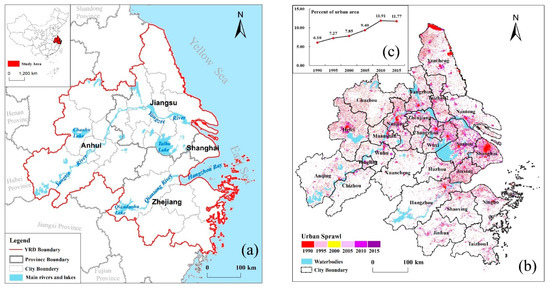
Figure 1.
(a) Location of the study area; (b) urban sprawl in the YRD from 1990 to 2015; (c) the variation of percent of urban area of the YRD from 1990 to 2015.
2.2. Methods
2.2.1. The Landscape Spatial Adjacency (LAdI) Formulation
(1) Definition of Landscape Spatial Adjacency
Landscape patches can be abstracted as polygons. Therefore, we used the concept of topological relationships to delimit the landscape spatial-adjacency relationship. Topological relationships are used to illustrate the relative position of spatial objects (in this case, polygons), and there are a variety of topological relationships between two objects, such as intersect, disjoint, contains, overlap, touch and cross, and so on [31]. Among them, contiguity is one of the basic spatial properties that describes whether a target object is a neighbor to other nontarget objects. Rook’s case (contiguity-edges-only) and Queen’s case (contiguity-edges-corners) are the two most common contiguity conceptualization models to illustrate the neighboring relationship between two polygons. In Rook’s case, only those polygons that share a common edge are considered as neighbors. In Queen’s case, polygons that share edges or have common corners can be regarded as neighbors [32]. In this study, the landscape spatial-adjacency relationship covers three types of topological relationships: (1) separation, polygons that have no common edges or have common corners are described as disjoint (Figure 2a); (2) contiguity, referring to Rook’s case mentioned above (Figure 2b); and (3) containment, when one polygon is within another polygon, which is a particular Rook’s case (Figure 2c). It is noted that polygons that share common corners are defined as separation in this study in that the length of the common edges of two landscape patches must be greater than zero if they are adjoining in the real-world scenario. Landscape spatial adjacency is characterized by asymmetry because the total perimeter and the patch number of different types of landscapes may not be equal all the time. That means the adjacency degree between target landscape A and nontarget landscape B is not always equal to that between target landscape B and nontarget landscape A (Figure 2c). To sum up, this study defines the landscape spatial-adjacency relationship as the neighboring relationship between two classes of landscape patches (namely, the target and nontarget), including separation, contiguity, and containment. The quantitative degree of spatial adjacency is determined by the length of the adjacent landscape edge and the number of adjacent landscape patches.
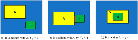
Figure 2.
The schematic diagram for spatial-adjacency relationships between target and nontarget landscape patches. If A is an urban landscape patch (target), and B is a natural landscape patch (nontarget), VB is the degree of spatial adjacency between landscape patch A and B. The red line in (b,c) represents the length of common edges between A and B, while (a) represents that there is no common edge between A and B. The blue background represents the spatial unit for analysis.
(2) LAdI at Class Level
In this study, we take urban landscape patches as our target landscape and natural landscape patches as our nontarget landscape. The class-level LAdI refers to the degree of spatial adjacency between the urban landscape and a particular natural landscape class in the study unit, thus representing the degree of potential ecological stress on that natural landscape class caused by urban expansion. The LAdI at class level can be computed for every class of natural landscapes in the study unit. The greater the LAdI at class level, the higher the potential impact of the urban landscape on natural landscapes, and the more vulnerable natural landscapes will be.
where Vi is the LAdI at class level of the natural landscape i, i refers to the class of the natural landscape, Li is the percent of the length of the adjacent landscape edge of the natural landscape i, Ui is the percent of the number of adjacent landscape patches of the natural landscape i, m is the patch number of the adjacent natural landscape (between the urban landscape and natural landscape i), k is the total patch number of the natural landscape i, lij is the length of common edges between the urban landscape and natural landscape patch ij, and Lig is the total length of the natural landscape patch ig. 0 ≤ m ≤ k.
(3) LAdI at the Landscape Level
Given spatial heterogeneity among different study units at the same scale; namely, the difference of landscape composition and configuration, we define the landscape-level LAdI as the average degree of spatial adjacency between the urban landscape and all classes of natural landscapes in the study unit, which represents the degree of integrated potential ecological stress on the regional natural landscape caused by urban expansion. The LAdI at landscape level is computed for an entire patch mosaic (namely, the whole study unit), and LAdI at class level should be computed for every class of natural landscapes in the study unit, so that the degrees of landscape spatial adjacency from study unit to unit could be comparable.
where LV is the LAdI at landscape level, Vi is the LAdI at class level of the natural landscape i, and n is the number of natural landscape classes in study area, which may vary from unit to unit. Theoretically, the value range of the LAdI (both LV and Vi) is (0,1). The larger the LAdI value is, the greater the degree of landscape spatial adjacency between the urban landscape and natural landscapes will be, and the less likely the natural landscape will spontaneously expand to the side of the urban landscape, because the intensity and frequency of human interference on regional ecosystems is usually greater than its natural restorative ability. In the case of Vi equal to one, this indicates all the natural landscape patches are surrounded by urban landscape, i.e., the containment case as shown in Figure 2c. There are two cases when Vi is equal to zero: one is where no urban landscape appears in the study unit; or where it appears, but only in the separation case illustrated in Figure 2a. In this case, the urban landscape will not have a direct impact on the disjoint natural landscape, and the disjoint natural landscape can spontaneously expand around or transform into other types of natural landscape. The other case is where the study unit is completely occupied by urban landscape, which means the area, length, and number of natural landscapes equal zero.
2.2.2. Urban Spatial-Expansion Index
There are various metrics applied to quantify the degree of urban expansion, such as the expansion area, speed, and acceleration of built-up [3]. In this study, we defined the urban spatial-expansion index as the percent of built-up area (PB), which equals the area of urban landscape divided by the total area of study unit. The value range of PB is (0,1). This study assumes that the area of urban landscape equals zero under the circumstance of no human interference. With the development of urban expansion, more and more natural landscapes are directly converted to urban landscape. Therefore, the greater the urban landscape encroachment on the natural landscape area, the higher the regional ecological stress.
where PB is the percent of built-up area; namely, the urban-expansion index. UA represents the area of urban landscape, Ai is the area of landscape type i, and N is the number of landscape classes, including urban landscape and natural landscapes (N = n + 1).
2.3. Data and Processing
In this study, the LAdI was calculated using land use and land cover data (LULC) with 30m spatial resolution from 1990 to 2015 in the YRD (source: National Earth System Science Data Sharing Infrastructure, National Science and Technology Infrastructure of China, http://www.geodata.cn (accessed on 19 March 2019)). The original 25 landscape classes of LULC data were reclassified as built-up, cultivated land, grassland, woodland, waterbodies, wetland, and unused land. According to the ecosystem service value of different landscapes [33], the seven landscape classes were further classified into urban landscape or natural landscape. The former refers to built-up, and the latter includes the rest of the six landscape classes mentioned above. As described previously, we took urban landscape as our target landscape and natural-landscape types as our nontarget landscape. Therefore, there were six landscape-adjacency types between urban landscape and natural landscape in this study; namely, the landscape-adjacency relationship between built-up and cultivated land, grassland, woodland, waterbodies, wetland, and unused land, respectively. We used shapefile data of the 26 cities’ boundaries in the YRD to delineate our municipal study unit, and 5 km-grid units within each municipal boundary. The 9008 5 km-grid units for analysis were generated based on the shapefile data of 26 cities’ boundary using the Fishnet tool in ArcGIS software.
Our quantitative assessment on regional ecological stress in the YRD comprised three steps: first, Python software was used to analyze the landscape spatial adjacency relationship between urban landscape and all types of natural landscapes based on LULC data to obtain the information about the landscape-adjacency types and corresponding attributes combined with spatial-analysis packages in ArcGIS, such as the length of the adjacent landscape edge and the number of adjacent landscape patches. Second, Vi, LV, and PB indexes at the 5 km-grid scale and municipal scale were calculated. In order to identify the distribution of vulnerable area that was greatly affected by urban expansion, the Vi values of each natural landscape class at the 5 km-grid scale were further divided into five grades by the equal interval of 0.2. Here, we defined the Vi value of natural landscape equal to or greater than 0.6 (Vi ≥ 0.6) as vulnerable natural landscape. Similarly, an LV value equal to or greater than 0.6 (LV ≥ 0.6) was defined as the vulnerable zone at the 5 km-grid scale. Moreover, the maximum Vi was observed for each city from 1990 to 2015 to assess the influence of different urbanization stages on variation in regional ecological stress due to urban spatial expansion over time. Finally, the relationship between PB and LV both at the municipal scale and the 5 km-grid scale were explored using scatter diagrams and Pearson correlation analysis.
3. Results
3.1. The Dynamics of the LAdI at the 5 km-Grid Scale
Based on LULC data, we calculated the LAdI at class level (Vi) for each 5 km-grid unit in the YRD from 1990 to 2015. Our results showed that among the six natural landscapes, cultivated land was most threatened by the expansion of urban landscape, followed by woodland, waterbodies, grassland, wetland, and unused land. Taking the year of 2015 as an example (for the variation maps of Vi for each natural landscape from 1990 to 2015, see Figures S1–S6), Figure 3 shows the totally different spatial distribution of Vi at the 5 km-grid scale for each natural landscape in the YRD in 2015. Specifically, the Vi of cultivated land was distributed almost throughout the YRD, with the Vi values for the northern area higher than those in the southern. The Vi of woodland and waterbodies were concentrated in the southern and northern YRD, respectively. The Vi of grassland, wetland, and unused land were scattered around the entire YRD, but with substantial grid cells possessing no Vi value.
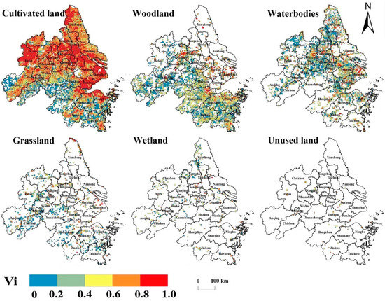
Figure 3.
The spatial variation of Vi at the 5 km-grid scale for each natural landscape in the YRD in 2015. The white grid cells indicate there was no common edge between the urban landscape and corresponding natural landscape.
Figure 4 shows the distribution of the vulnerable natural landscapes in the YRD from 1990 to 2015, through merging the 5 km-grid units with the Vi value of each class of natural landscape equal to or greater than 0.6 into a united map. Our results showed the vulnerable natural landscapes were mainly distributed in the north of the YRD from 1990 to 2015, including Shanghai and most of the cities in Jiangsu and Anhui Provinces. There was no substantial change in the spatial pattern of the vulnerable natural landscapes before 2010. However, after that, the vulnerable area (the number of 5 km-grid cells) of woodland and waterbodies showed an increasing trend along the Yangtze River and Hangzhou Bay, especially in the area east of Taihu Lake. Overall, the number of grid cells containing vulnerable natural landscapes showed an increasing trend year by year (Figure 5). This reflects the increasing extent of natural landscapes affected by urban landscape expansion. The percent of the grid numbers of vulnerable cultivated land in the total grid numbers of the YRD (9008) increased from 44.99% in 1990 to 49.89% in 2015, with the highest increase of 4.90% among the six classes of natural landscapes.
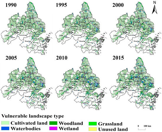
Figure 4.
The spatial variation in the vulnerable landscape in the YRD from 1990 to 2015 (Vi ≥ 0.6 for all classes of natural landscape). The white grid cells indicate there was no common edge between the urban landscape and corresponding natural landscape.
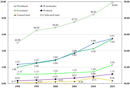
Figure 5.
The percent of the grid numbers of vulnerable landscape in the total grid numbers of the YRD from 1990 to 2015 (Vi ≥ 0.6 for all kinds of natural landscapes). Cultivated land was on a secondary y-axis because of the scale differences compared with other natural landscapes.
Furthermore, we calculated LV at the 5 km-grid scale to analyze the integrated potential ecological stress in each grid cell caused by urban expansion. Figure 6 illustrates the spatial variation of LV at the 5 km-grid scale in the YRD from 1990 to 2015. The vulnerable zones were mainly distributed in the urbanized area along the Yangtze River and Hangzhou Bay. The vulnerable zone (where LV ≥ 0.6) gradually expanded outward from the downtown area of each city. Grids with an LV value greater than 0.4 but less than 0.6 also substantially increased along the Yangtze River and Hangzhou Bay, showing a trend of expansion from north to south of the YRD. The percent of grid cells in which the LV value was greater than 0.4 but less than 0.6 increased from 16.22% in 1990 to 20.78% in 2015, with a total increase of 4.56% (see Figure S7).
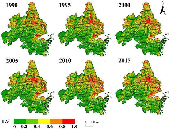
Figure 6.
The spatial variation of LV at the 5 km-grid scale in the YRD from 1990 to 2015. The white grid cells indicate there was no common edge between the urban landscape and natural landscapes.
3.2. The Dynamics of the LAdI at the Municipal Scale
We calculated Vi at the municipal scale to identify the most vulnerable natural landscape for each city. Figure 7 illustrates the maximum value of Vi (Vimax) and the corresponding most vulnerable natural landscape for each city in each period.
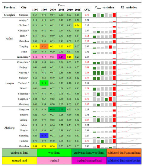
Figure 7.
The maximum value of Vi (Vimax) and the corresponding natural landscape for each city in the YRD from 1990 to 2015. The asterisks in the second column denote the 12 cities where the total area of urban landscape decreased slightly in 2015 compared with that in 2010. AVG equals to the average of Vimax for each city from 1990 to 2015. The bars in the Vimax variation illustrate the corresponding maximum Vi observed for each city from 1990 to 2015.The green and red bars represent the minimum and maximum values of Vimax over these years, respectively. PB variation illustrated a changing trend in PB for each city over time.
It is obvious that cultivated land is the most vulnerable natural landscape in most cities in the YRD from 1990 to 2015, especially the cities located in Shanghai and Jiangsu Provinces. Specifically, the Vi value of cultivated land in 19 of 26 cities in the YRD in each period was greater than that of other classes of natural landscape, among which the average Vimax value of cultivated land in 25 years of 13 cities was greater than 0.53. For the remaining seven cities (including Chizhou, Tongling, and Xuancheng in Anhui Province; Hangzhou, Shaoxing, and Zhoushan in Zhejiang Province; and Taizhou1 in Jiangsu Province), the most vulnerable natural landscape varied. For instance, the most vulnerable natural landscape in Zhoushan was unused land from 1990 to 2000, but was cultivated land from 2000 to 2015. As for Hangzhou, cultivated land in Hangzhou has been the most vulnerable natural landscape since 1990, and its Vimax value has been increasing year by year. Meanwhile, urban expansion in Hangzhou also exerted substantial ecological stress on woodland from 2000 to 2005, when the Vi values of woodland were equal to those of cultivated land. As for Xuancheng, the natural landscape that was the most vulnerable showed a gradual change from wetland and unused land to cultivated land since 1990. The Vimax values of 25 out of 26 cities showed an increasing trend year by year, except for Zhoushan.
Comparing the Vimax value for each year among 26 cities, cultivated land in Nantong and Jiaxing was most vulnerable because both these two cities showed continual high-intensity ecological stress on cultivated land from 1990 to 2015, with an average Vimax value of cultivated land in 25 years greater than 0.84. By contrast, the Vimax values of Chizhou, Xuancheng, and Taizhou1 were less than 0.2, which means that all classes of natural landscapes in these three cities were less threatened by urban expansion, and did not reach the critical value of 0.6. Besides, compared with the Vimax value of each city year on year, the Vimax value of 23 cities (except for Zhoushan, Yangzhou, and Tongling) appeared in 2015, although the total area of urban landscape in 12 of 23 cities decreased slightly in 2015 compared with that in 2010. That means decreasing urban area does not result in less ecological stress all the time.
3.3. Comparison between the LAdI and the Urban-Expansion Index
The Pearson correlation method was applied to analyze the correlation between the LAdI at landscape level (LV) and the urban-expansion index (PB). The results (Table 1) showed that LV and PB had a significant positive correlation at both the municipal and 5 km-grid scales. The mean values of their correlation coefficients were 0.81 and 0.62 (0.57, with the grid cells of PB value equal to 0 or 1 excluded), respectively. Furthermore, when drawing the scatter diagrams between LV and PB from 1990 to 2015, we found that the scatters at the 5 km-grid scale were concentrated in the upper left of the diagonal line of scatter diagrams in Figure 8. This indicates that there were multiple LVs with different values corresponding to one PB with the same value at the 5 km-grid scale; i.e., the study units with the same percent of built-up area may have had different landscape-adjacency degrees.

Table 1.
The correlation between LV and PB at the municipal scale and the 5 km-grid scale in the YRD from 1990 to 2015.
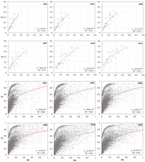
Figure 8.
Scatter diagrams between LV and PB at the municipal scale and the 5 km-grid scale in the YRD from 1990 to 2015. When 0 < PB < 1, the functional relationship between LV and PB fitted a power-exponential growth curve well.
Regression analysis was applied to further explore the function relationship between LV and PB. Theoretically, the value of PB ranges from 0 to 1, but it is impossible for PB at the municipal scale to reach 0 and 1. In order to control the consistency of the PB value range at the 5 km-grid and municipal scales, the grid cells with a PB value equal to 0 or 1 were excluded from the regression analysis. The results showed that the functional relationship between LV and PB could be described as a power-exponential growth curve, and the fitting coefficients (R2) at the municipal scale were better than those at the 5 km-grid scale, indicating that when PB is greater than 0 and less than 1, the greater the PB, the greater the LV.
4. Discussion
4.1. The Implications of the LAdI
In this study, the LAdI at the class level (Vi) and landscape level (LV) were defined to quantify the ecological stress for an individual natural landscape and an entire landscape mosaic subjected to an urban landscape, respectively. Then, the vulnerable landscapes (Vi ≥ 0.6) and vulnerable zones (LV ≥ 0.6) were extracted based on the critical value of the LAdI. Our analyses supported the arguments that the spatial-adjacency relationship between urban landscape and natural landscape is different, both within the individual landscape type and among different landscape types, and urban spatial expansion will impact the spatial-adjacency relationship between the urban landscape and natural landscapes. Correspondingly, two specific implications of the LAdI can be concluded as following from the case study.
The LAdI can effectively reflect the spatial-adjacency relationship between the urban landscape and natural landscape. The closer the natural landscapes are to urban landscape, the higher the LAdI value. O’Neil et al. (1988) deemed that the values of a useful index should be reasonably distributed across the potential range of the index to provide maximum discrimination and perform well in discriminating the geographic distribution of landscape-pattern types [26]. By analysis of the dynamics of the LAdI at the 5 km-grid scale, it was found that there was obvious spatial heterogeneity in the landscape spatial-adjacency relationship both within the individual landscape type and among different landscape types (Figure 3). The case study in the YRD showed that cultivated land in the northern YRD was more vulnerable than that in the southern, and it was the most vulnerable landscape among six natural landscapes in the YRD from 1990 to 2015. Combined with LULC data from 1990 to 2015 (Figure S8), it can be seen that cultivated land was mainly distributed in the northern YRD, and urban-landscape expansion was achieved mainly through encroaching on cultivated land, resulting in a close adjacency relation between the urban landscape and cultivated land. Therefore, the LAdI is a useful index to characterize the landscape pattern in term of the spatial-adjacency relationship.
The LAdI can comprehensively reflect the impact of urban spatial expansion on a neighboring natural landscape. The larger the urban landscape, the more likely the natural landscape patches will be adjacent to urban landscape, and the greater the ecological stress of urban landscape on natural landscapes. However, decreasing urban area does not result in less ecological stress all the time. By comparing the spatial pattern of the vulnerable landscapes and vulnerable zones from 1990 to 2015, it was found that the extent of the vulnerable landscapes and vulnerable zones was increased with the urban expansion. The case study in the YRD showed that the vulnerable zones were mainly distributed in the urbanized area along the Yangtze River and Hangzhou Bay, and gradually expanded outward from the downtown area of each city, which was consistent with the spatial pattern of urban-landscape expansion in the YRD as shown in Figure 1b. Similarly, the results of the dynamics of the LAdI at the municipal scale showed that cultivated land was the most vulnerable landscape for most cities, and the ecological stress on cultivated land kept increasing, which was in line with the results at the 5 km-grid scale, as shown in Figure S1. This indicated that the dynamics of ecological stress in the YRD quantified by the LAdI were consistent with the dynamics of urbanization at both the small and large scales. Nevertheless, it was unexpected to find that the ecological stress on cultivated land (the Vimax as shown in Figure 7) kept increasing in 12 cities, although the PB of them decreased slightly from 2010 to 2015. This means that urban sprawl or urban renewal has continued in these cities even though the total urban area decreased, and the LAdI was sensitive enough to identify this variation in urban morphology.
4.2. Comparison between the Edge-Based Index (LAdI) and the Area-Based Index (PB)
When comparing the LAdI with the PB, we found that these two indexes were related but fundamentally different. Density analysis is basic and important for urban expansion studies, and the built-up density (namely PB) is one of the most common density metrics to measure the degree of urban expansion [34].The correlation analysis in Section 3.3 showed that the LV had a significant positive correlation with the PB.This implies that the LAdI could also characterize the degree of urban expansion. Nevertheless, they cannot be replaced by each other. There are three main differences between the LAdI and the PB: (1) The ecological stress they illustrated is different. The PB represents the area loss of habitats encroached by urban landscape. TheLAdI represents the potential impacts on species and ecosystems induced by human disturbance appearing along the common edges. For instance, habitats for birds next to urban areas are likely to suffer from noise and night pollution [29]. (2) The PB is an area-based index, while the LAdI is an edge-based index. Although both of these indexes can be calculated using LULC data, the PB is built in terms of the area of urban landscape, while the LAdI is built in terms of the common edges between the urban landscape and natural landscapes, and considers both the change of adjacent edge length and the number of adjacent patches. (3) The LAdI could express more information than the PB. The LAdI can not only quantify the degree of the potential regional ecological stress caused by urban expansion at the landscape level, but also can illustrate this at class level for individual natural landscape.
Furthermore, we found that the landscape-adjacency degree showed significant differences, even though the urban-expansion index was the same at the 5 km-grid scale, showing multiple values of LV corresponding to a single value of PB (Figure 8). This could be attributed to the difference in landscape patterns among grid cells. This finding will greatly contribute to distinguishing the regional ecological stress among cities or study units with the same degree of urban expansion, but under different patterns of urban expansion to characterize urban expansion in detail. Especially when the total urban area of a city is under control or inventory planning, subtle changes to the inner urban area caused by the adjustment of urban-landscape configuration will become quantifiable, comparable, and monitored. For instance, from 2010 to 2015, the urban landscape in the YRD was in a stable expansion stage when the total urban area in the YRD decreased, but new urban area appeared in most cities, resulting in the maximum Vimax of 23 cities (except for Zhoushan, Yangzhou, and Tongling) appearing in 2015. This indicates that the ecological stress on ecosystems kept increasing. However, it is easy to draw an incorrect conclusion that ecological stress decreased merely according to the numerical variation of the PB in this period. In the process of urbanization, the regional ecological stress of the urban landscape on natural landscape is manifested as not only the direct area encroachment [17], but also the adjacency effect [35]. Considering all the above, we suggest that both the area-based index PB and the edge-based index LAdI should be taken into account when evaluating the regional ecological stress due to urban sprawl.
4.3. Future Works and Applications of the LAdI
As with previous landscape metrics, LAdI can be conveniently calculated based on a categorical map. Therefore, the effectiveness of the description for the landscape-adjacency relationship greatly depends on the map accuracy (spatial resolution of data) and the classification accuracy (the number of identifiable landscape types) of LULC data. It is certain that the development of high-resolution remote-sensing technology makes it possible to identify landscape types and landscape boundaries more accurately and elaborately, and consequently provides data support for more accurate identification of various landscape-adjacent relationships. In this study, the LAdI was applied at both a small scale (5 km-grid) and a large scale (city) to assess the regional ecological stress due to urbanization based on LULC data with a 30 m spatial resolution. In future studies, we will further explore the scale effect of the landscape-adjacency index.
In addition, the further implications of the LAdI and its influencing mechanism require further study. It is critical to develop landscape metrics related to ecological processes [36]. This study developed the LAdI to link urban expansion with ecological stress on ecosystems. It was found that there was a significant nonlinear relationship (power-exponential growth curve) between the PB and LV. Generally, the grids with a high LV value were mainly concentrated in the main urban area. Therefore, we assumed that this may be attributed to the differences in urban-expansion patterns in highly urbanized areas, but the influence mechanism of urban-expansion patterns on the LAdI need to be further studied. Besides, LAdI can also be used to describe the variation of landscape spatial-adjacency relationships induced by other factors, such as desertification, salinization threat to urban and natural landscapes [37], cropland expansion [38], wetland reclamation [39], etc. However, considering the asymmetry of landscape spatial adjacency as mentioned in Section 2.2.1, the specific implications of landscape spatial adjacency should be further explored in combination with the study aims.
5. Conclusions
From the perspective of the spatial-adjacency relationship between the urban and natural landscapes, this study proposed a novel edged-based index (LAdI) at the class level (Vi) and landscape level (LV) to assess the regional ecological stress caused by urban expansion. Taking the Yangtze River Delta Urban Agglomerations as the study area, the spatiotemporal evolution characteristics of the vulnerable natural landscapes/zones from 1990 to 2015 in the YRD were identified in detail through Vi and LV at the 5 km-grid scale, and the most vulnerable natural landscapes for 26 cities in different urbanization stages were rapidly diagnosed through Vi at the municipal scale. Our results showed that the vulnerable zones were mainly distributed in the north of the YRD, and cultivated land was the most vulnerable natural landscape under the stress of urban expansion, because the urban expansion in the YRD, especially in the northern YRD, was achieved mainly through encroaching on cultivated land from 1990 to 2015. The most vulnerable natural landscapes of the 26 cities in different periods were different, among which 19 cities were dominantly characterized as cultivated land in each period, and the remaining seven cities varied year by year. Furthermore, by comparing with the urban-expansion index (PB), this study analyzed the difference and relationship between the edge-based index LAdI and the area-based index PB. We found that the LAdI at the landscape level (LV) and the PB had a significant positive correlation at both the municipal and 5 km-grid scales, indicating that both indexes could represent the degree of urban expansion. However, compared to the PB, the LAdI could not only depict the influence of urban expansion on landscape-adjacency relationships in more detail, but more importantly, it makes regional ecological stresses under different urban-sprawl patterns, but with the same percent of built-up areas, comparable. To sum up, the landscape-adjacency index provides a new perspective and a new method to quantify characterization of urban sprawl. We suggest that both the area-based index PB and the edge-based index LAdI should be considered when assessing the regional ecological stress caused by urban sprawl, considering that the change of land-use area, length of adjacent edges, and the number of adjacent patches may take place simultaneously in the process of urbanization.
Supplementary Materials
The following are available online at https://www.mdpi.com/article/10.3390/rs13071352/s1, Figure S1–S6: the spatial variation of Vi at 5 km-grid scale in YRD from 1990 to 2015 for cultivated land, woodland, waterbodies, wetland, grassland, and unused land, respectively, Figure S7: the percent of the grid number of different LV grading in the total grid number of YRD from 1990 to 2015, Figure S8: land use and land cover change in YRD from 1990 to 2015.
Author Contributions
Conceptualization, M.L. and T.L.; methodology, M.L. and T.L.; software, M.L.; validation, X.L. (Xiaofang Liu); formal analysis, M.L. and L.X.; investigation, L.X. and J.S.; resources, M.L., J.Z. and Y.L.; writing—original draft preparation, M.L. and T.L.; writing—review and editing, M.L., T.L. and L.J.; visualization, M.L.; project administration, H.Y., G.Z., X.L. (Xin Lu) and T.L.; funding acquisition, T.L. All authors have read and agreed to the published version of the manuscript.
Funding
This research was funded by the National Key Research & Development Program of China, grant number 2016YFC0502702.
Institutional Review Board Statement
Not applicable.
Informed Consent Statement
Not applicable.
Data Availability Statement
The data presented in this study are available on request from the corresponding author.
Acknowledgments
The authors are grateful for the support of the National Key Research & Development Program of China (2016YFC0502702). We are also grateful to reviewers for their helpful comments and suggestions for improving the manuscript.
Conflicts of Interest
The authors declare no conflict of interest.
References
- Grimm, N.B.; Faeth, S.H.; Golubiewski, N.E.; Redman, C.L.; Wu, J.; Bai, X.; Briggs, J.M. Global change and the ecology of cities. Science 2008, 319, 756–760. [Google Scholar] [CrossRef] [PubMed]
- Seto, K.C.; Fragkias, M.; Güneralp, B.; Reilly, M.K. A meta-analysis of global urban land expansion. PLoS ONE 2011, 6, e23777. [Google Scholar] [CrossRef]
- Wang, L.; Jia, Y.; Li, X.; Gong, P. Analysing the driving forces and environmental effects of urban expansion by mapping the speed and acceleration of built-up areas in china between 1978 and 2017. Remote Sens. 2020, 12, 3929. [Google Scholar] [CrossRef]
- David, P.; Annemarie, S. A critical look at representations of urban areas in global maps. GeoJournal 2007, 69, 55–80. [Google Scholar]
- Liu, Z.; He, C.; Zhou, Y.; Wu, J. How much of the world’s land has been urbanized, really? A hierarchical framework for avoiding confusion. Landsc. Ecol. 2014, 29, 763–771. [Google Scholar] [CrossRef]
- Hahs, A.K.; McDonnell, M.J.; McCarthy, M.A.; Vesk, P.A.; Corlett, R.T.; Norton, B.A.; Clemants, S.E.; Duncan, R.P.; Thompson, K.; Schwartz, M.W. A global synthesis of plant extinction rates in urban areas. Ecol. Lett. 2009, 12, 1165–1173. [Google Scholar] [CrossRef]
- McDonald, R.I.; Mansur, A.V.; Ascensão, F.; Colbert, M.; Crossman, K.; Elmqvist, T.; Gonzalez, A.; Güneralp, B.; Haase, D.; Hamann, M.; et al. Research gaps in knowledge of the impact of urban growth on biodiversity. Nat. Sustain. 2019, 3, 16–24. [Google Scholar] [CrossRef]
- Pereira, H.M.; Leadley, P.W.; Proença, V.; Alkemade, R.; Scharlemann, J.P.W.; Fernandez-Manjarrés, J.F.; Araújo, M.B.; Balvanera, P.; Biggs, R.; Cheung, W.W.L.; et al. Scenarios for global biodiversity in the 21st century. Science 2010, 330, 1496–1501. [Google Scholar] [CrossRef] [PubMed]
- Alberti, M. The effects of urban patterns on ecosystem function. Int. Reg. Sci. Rev. 2005, 28, 168–192. [Google Scholar] [CrossRef]
- Liang, Y.; Liu, L. Simulating land-use change and its effect on biodiversity conservation in a watershed in northwest China. Ecosyst. Health Sustain. 2017, 3, 1335933. [Google Scholar] [CrossRef]
- Alberti, M.; Marzluff, J.M. Ecological resilience in urban ecosystems: Linking urban patterns to human and ecological functions. Urban Ecosyst. 2004, 7, 241–265. [Google Scholar] [CrossRef]
- Elmqvist, T.; Fragkias, M.; Goodness, J.; Güneralp, B.; Marcotullio, P.J.; McDonald, R.I.; Parnell, S.; Schewenius, M.; Sendstad, M.; Seto, K.C.; et al. Urbanization, Biodiversity And Ecosystem Services: Challenges And Opportunities. Available online: http://tailieuso.tlu.edu.vn/handle/DHTL/5103 (accessed on 21 May 2019).
- Noori, N.; Kalin, L.; Sen, S.; Srivastava, P.; Lebleu, C. Identifying areas sensitive to land use/land cover change for downstream flooding in a coastal Alabama watershed. Reg. Environ. Chang. 2016, 16, 1833–1845. [Google Scholar] [CrossRef]
- Phelan, P.E.; Kaloush, K.; Miner, M.J.; Golden, J.S.; Phelan, B.; Silva, H.R.; Taylor, R.A. Urban heat island: Mechanisms, implications, and possible remedies. Annu. Rev. Environ. Resour. 2015, 40, 285–307. [Google Scholar] [CrossRef]
- Walz, U.; Syrbe, R.-U. Landscape indicators—Monitoring of biodiversity and ecosystem services at landscape level. Ecol. Indic. 2018, 94, 1–5. [Google Scholar] [CrossRef]
- Lin, T.; Ge, R.; Huang, J.; Zhao, Q.; Lin, J.; Huang, N.; Zhang, G.; Li, X.; Ye, H.; Yin, K. A quantitative method to assess the ecological indicator system’s effectiveness: A case study of the Ecological Province Construction Indicators of China. Ecol. Indic. 2016, 62, 95–100. [Google Scholar] [CrossRef]
- Peng, J.; Tian, L.; Liu, Y.; Zhao, M.; Hu, Y.; Wu, J. Ecosystem services response to urbanization in metropolitan areas: Thresholds identification. Sci. Total Environ. 2017, 607–608, 706–714. [Google Scholar] [CrossRef]
- Li, P.; Cao, H. Comprehensive assessment on the ecological stress of rapid land urbanization per proportion, intensity, and location. Ecosyst. Health Sustain. 2019, 5, 242–255. [Google Scholar] [CrossRef]
- Güneralp, B.; Perlstein, A.S.; Seto, K.C. Balancing urban growth and ecological conservation: A challenge for planning and governance in China. Ambio 2015, 44, 532–543. [Google Scholar] [CrossRef]
- Lu, D.; Xu, X.; Tian, H.; Moran, E.; Zhao, M.; Running, S. The effects of urbanization on net primary productivity in Southeastern China. Environ. Manag. 2010, 46, 404–410. [Google Scholar] [CrossRef]
- Peng, J.; Shen, H.; Wu, W.; Liu, Y.; Wang, Y. Net primary productivity (NPP) dynamics and associated urbanization driving forces in metropolitan areas: A case study in Beijing City, China. Landsc. Ecol. 2016, 31, 1077–1092. [Google Scholar] [CrossRef]
- Tan, J.; Li, A.; Lei, G.; Bian, J.; Zhang, Z. A novel and direct ecological risk assessment index for environmental degradation based on response curve approach and remotely sensed data. Ecol. Indic. 2019, 98, 783–793. [Google Scholar] [CrossRef]
- Liu, X.; Huang, Y.; Xu, X.; Li, X.; Li, X.; Ciais, P.; Lin, P.; Gong, K.; Ziegler, A.D.; Chen, A.; et al. High-spatiotemporal-resolution mapping of global urban change from 1985 to 2015. Nat. Sustain. 2020, 3, 564–570. [Google Scholar] [CrossRef]
- Zhang, Q.; Seto, K.C. Mapping urbanization dynamics at regional and global scales using multi-temporal DMSP/OLS nighttime light data. Remote Sens. Environ. 2011, 115, 2320–2329. [Google Scholar] [CrossRef]
- Biondini, M.; Kandus, P. Transition matrix analysis of land-cover change in the accreation area of the lower delta of the Parana River(Argentina) reveals two succession pathways. Wetlands 2006, 26, 981–991. [Google Scholar] [CrossRef]
- O’Neillr, R.V.; Krummel, J.R.; Gardner, R.H.; Sugihara, G.; Jackson, B.; DeAngelist, D.L.; Milne, B.T.; Turner, M.G.; Zygmunt, B.; Christensen, S.W.; et al. Indices of landscape pattern. Landsc. Ecol. 1988, 1, 153–162. [Google Scholar]
- Hodgson, J.A.; Moilanen, A.; Wintle, B.A.; Thomas, C.D. Habitat area, quality and connectivity: Striking the balance for efficient conservation. J. Appl. Ecol. 2010, 48, 148–152. [Google Scholar] [CrossRef]
- Seto, K.C.; Fleishman, E.; Fay, J.P.; Betrus, C.J. Linking spatial patterns of bird and butterfly species richness with Landsat TM derived NDVI. Int. J. Remote Sens. 2004, 25, 4309–4324. [Google Scholar] [CrossRef]
- Senzaki, M.; Barber, J.R.; Phillips, J.N.; Carter, N.H.; Cooper, C.B.; Ditmer, M.A.; Fristrup, K.M.; McClure, C.J.W.; Mennitt, D.J.; Tyrrell, L.P.; et al. Sensory pollutants alter bird phenology and fitness across a continent. Nat. Cell Biol. 2020, 587, 605–609. [Google Scholar] [CrossRef] [PubMed]
- Hersperger, A.M. Spatial adjacencies and interactions: Neighborhood mosaics for landscape ecological planning. Landsc. Urban Plan. 2006, 77, 227–239. [Google Scholar] [CrossRef]
- Di Felice, P.; Clementini, E.; Hinterberger, H.; Domingo-Ferrer, J.; Kashyap, V.; Khatri, V.; Snodgrass, R.T.; Terenziani, P.; Koubarakis, M.; Zhang, Y.; et al. Topological relationships. In Encyclopedia of Database Systems; Metzler, J.B., Ed.; Springer: Cambridge, UK, 2009. [Google Scholar]
- Grekousis, G. Think Spatially; Cambridge University Press (CUP): Cambridge, UK, 2020; pp. 1–58. Available online: https://doi.org/10.1017/9781108614528.002 (accessed on 23 May 2020).
- Costanza, R.; D’Arge, R.; De Groot, R.; Farber, S.; Grasso, M.; Hannon, B.; Limburg, K.; Naeem, S.; ONeill, R.V.; Paruelo, J.; et al. The value of the world’s ecosystem services and natural capital. Nature 1997, 387, 253–260. [Google Scholar] [CrossRef]
- Jiao, L. Urban land density function: A new method to characterize urban expansion. Landsc. Urban Plan. 2015, 139, 26–39. [Google Scholar] [CrossRef]
- Lin, M.; Lin, T.; Sun, C.; Jones, L.; Sui, J.; Zhao, Y.; Liu, J.; Xing, L.; Ye, H.; Zhang, G.; et al. Using the Eco-Erosion Index to assess regional ecological stress due to urbanization—A case study in the Yangtze River Delta urban agglomeration. Ecol. Indic. 2020, 111, 106028. [Google Scholar] [CrossRef]
- Wu, J.; Hobbs, R. Key issues and research priorities in landscape ecology: An idiosyncratic synthesis. Landsc. Ecol. 2002, 17, 355–365. [Google Scholar] [CrossRef]
- Jiao, Y.; Xiao, D. Spatial neighboring characteristics among patch types in oasis and its ecological security. Chin. J. Appl. Ecol. 2004, 15, 31–35. (In Chinese) [Google Scholar]
- Eigenbrod, F.; Beckmann, M.; Dunnett, S.; Graham, L.; Holland, R.A.; Meyfroidt, P.; Seppelt, R.; Song, X.; Spake, R.; Václavík, T.; et al. Identifying agricultural frontiers for modeling global cropland expansion. One Earth 2020, 3, 504–514. [Google Scholar] [CrossRef] [PubMed]
- Hou, X.; Feng, L.; Tang, J.; Song, X.; Liu, J.; Zhang, Y.; Wang, J.; Xu, Y.; Dai, Y.; Zheng, C.; et al. Anthropogenic transformation of Yangtze Plain freshwater lakes: Patterns, drivers and impacts. Remote Sens. Environ. 2020, 248, 111998. [Google Scholar] [CrossRef]


Publisher’s Note: MDPI stays neutral with regard to jurisdictional claims in published maps and institutional affiliations. |
© 2021 by the authors. Licensee MDPI, Basel, Switzerland. This article is an open access article distributed under the terms and conditions of the Creative Commons Attribution (CC BY) license (https://creativecommons.org/licenses/by/4.0/).