Article

Quantifying the Cooling Effect and Scale of Large Inner-City Lakes Based on Landscape Patterns: A Case Study of Hangzhou and Nanjing

1
Institute of Remote Sensing and Earth Sciences, College of Science, Hangzhou Normal University, Hangzhou 311121, China
2
Faculty of Geo-Information Science and Earth Observation (ITC), University of Twente, 7500AE Enschede, The Netherlands
3
Faculty of Life and Environmental Sciences, University of Tsukuba, 1-1-1 Tennodai, Tsukuba City, Ibaraki 305-8572, Japan
*
Author to whom correspondence should be addressed.
Remote Sens. 2021, 13(8), 1526; https://doi.org/10.3390/rs13081526
Submission received: 16 March 2021 / Revised: 10 April 2021 / Accepted: 13 April 2021 / Published: 15 April 2021
(This article belongs to the Special Issue Geographical Analysis and Modeling of Urban Heat Island Formation)

Abstract

:
The rapid urbanization worldwide has brought various environmental problems. The urban heat island (UHI) phenomenon is one of the most concerning issues because of its strong relation with daily lives. Water bodies are generally considered a vital resource to relieve the UHI. In this context, it is critical to develop a method for measuring the cooling effect and scale of water bodies in urban areas. In this study, West Lake and Xuanwu Lake, two famous natural inner-city lakes, are selected as the measuring targets. The scatter plot and multiple linear regression model were employed to detect the relationship between the distance to the lake and land surface temperature based on Landsat 8 Operational Land Imager/Thermal Infrared Sensor (OLI/TIRS) and Sentinel-2 data. The results show that West Lake and Xuanwu Lake massively reduced the land surface temperature within a few hundred meters (471 m for West Lake and 336 m for Xuanwu Lake) and have potential cooling effects within thousands of meters (2900 m for West Lake and 3700 m for Xuanwu Lake). The results provide insights for urban planners to manage tradeoffs between the large lake design in urban areas and the cooling effect demands.

Graphical Abstract

1. Introduction

Due to the rapid urbanization and high-density population, various environmental changes occurred in urban areas [1]. The urban heat island (UHI) is one of the most significant climate changes caused by human activities [2]. UHI, firstly mentioned by Howard [3], refers to the common phenomenon in which the temperatures in urban areas are higher than that in the surrounding non-urbanized areas [4]. The high temperatures caused by the UHI phenomenon not only change the local climate environment resulting in extreme weather conditions [5], increased energy and water consumption [6,7], but also raise the risk of human health issues [8,9]. Thus, UHI mitigation strategies should be studied and incorporated into future city design and planning to reduce the adverse effects.
UHI represents the temperature difference between urban and suburban areas [10]. There are mainly three ways to measure the temperature for UHI studies, including meteorological station observation records [11,12], thermometers mounted on vehicles [13], and remote sensing observation of the surface temperature [14,15,16]. Among them, the meteorological stations provide detailed records but fail to show the spatial distribution characteristics of the temperature on a large scale. The vehicle’s temperature records are limited in space and biased since the readings are made on the spot where the equipment is situated [17]. The land surface temperature (LST) derived from remote sensing observations provides easy access and large-scale temperature data and gradually becomes the primary way to assess the UHI effect [18,19]. For example, Khorchani et al. explored the temporal and spatial distributing characteristics of LST in peninsular Spain based on advanced very high resolution radiometer (AVHRR) data [20]. Clinton and Gong used the moderate resolution imaging spectroradiometer (MODIS) sensor to obtain global surface temperature and surface greenness at 1 km resolution [19]. Chen et al. utilized the Landsat thematic mapper (TM) and enhanced thematic mapper plus (ETM+) thermal infrared (TIR) data with 120 m and 60 m spatial resolutions, respectively, for local-scale studies of UHI [21]. Satellite-derived LST measurements have been conducted primarily by MODIS [18,19,22] and AVHRR data for large-scale regional (including national, continental, and even global) LST studies [23]. On the other hand, Landsat data provide better resolution and less frequent LST observations, and have been widely used in city-level studies [17].
Urbanization changes the surface temperature in cities by modifying the characteristics of the natural surface [24]. Landscape composition and configuration are considered two main factors in LST variation [25,26,27,28]. Of these impact factors, large water bodies in urban areas (e.g., lakes, rivers, and streams) are regarded as an effective resource to reduce the UHI [29]. The specific heat capacity of water bodies is more remarkable than other materials [30]. Thus, they have a lower warming-up speed than the surrounding areas, resulting in “cool islands” during the daytime [31]. Urban lakes play a significant role in regional climate regulation, maintenance of ecosystem balance, and diversification of urban derivatives [32]. Thus, it is crucial to quantitatively evaluate the cooling effects of the urban lakes and determine their cooling scale. In previous studies, the distances-LST scatter diagram has been widely used to qualitatively describe the cooling effects of lakes [25,33]. However, the cooling effects of the lake can be affected by surrounding land covers (e.g., trees, grasses, buildings and pavements) and the urban landscape patterns [11]. It is still a lack of explicit discussion on the impact of surrounding urban landscape patterns on the urban lake cooling effect. To bridge this knowledge gap, this article proposed a scientific method to assess the urban lake cooling effects and the potential cooling effect scale based on multiple linear regression methods by considering the urban landscape patterns surrounding the lakes with multi-source remote sensing images.
Here, two famous Lakes (West Lake in Hangzhou, Zhejiang province; Xuanwu Lake in Nanjing, Jiangsu province) were selected as the targets to quantitatively evaluate the cooling effect of the large natural inner-city lakes by considering their surrounding landscape patterns. West Lake, located in Hangzhou, is among the 55 United Nations Educational, Scientific and Cultural Organization (UNESCO) World Heritage sites in China [34]. Xuanwu Lake, the largest imperial garden lake in China, is located in Nanjing. As two of the highest gross domestic product (GDP) capitals of provinces, Hangzhou and Nanjing suffer from high temperatures during summer. Both of them are listed in the top 10 hottest cities in China (http://www.cma.gov.cn/) (accessed on 26 January 2021). As the landmarks of the two cities, West Lake and Xuanwu Lake are regarded as the typical inner-city lakes to detect the cooling scale of water bodies in cities.
This study aims to quantify the cooling effect and scale of urban lakes based on landscape patterns and provide important insights on landscape design and urban planning in the perspective of relieving UHI intensity. To achieve the primary purpose, the study has three sub-objectives, including (1) detect the variables affecting the LST in the surrounding areas of the urban lake; (2) build the regression models for LST in different scales; and (3) determine the cooling scale and the corresponding importance of lake for relieving the LST in the neighborhoods.

2. Materials and Methods

2.1. Study Area

Hangzhou, the capital of Zhejiang province, is situated in the southern wing of the Yangtze River Delta, with a latitude of 29°11′ N to 30°34′ N and a longitude of 118°20’ E to 120°37′ E) (Figure 1). Hangzhou has a subtropical monsoon climate with clearly divided four seasons. Hangzhou owns the natural environment that integrates rivers, lakes, and hills. As one of the three core cities (Shanghai, Nanjing, and Hangzhou) in the Yangtze River Delta urban agglomerations, Hangzhou boasts a population of 10.36 million and steady economic growth of a local GDP of RMB 1.54 trillion in 2019 [35]. The world-famous scenic spot, West Lake, lies in Hangzhou city’s main urban area, 1.4 km away from the city center (Wulin Square). It is an oval-shaped lake covering a water area of 6.38 km2, with its three sides surrounded by the mountains, one side by the urban area. The bottom of West Lake is relatively flat, with an average water depth of 2.27 m.
As the capital of Jiangsu province, Nanjing is located at the lower reaches of the Yangtze River (31°14′ N–32°37′ N, 118°22′ E–119°14′ E) (Figure 1). Nanjing is in the monsoon climate area of the north subtropical zone, with four distinct seasons. In terms of topographic conditions, Nanjing is connected with the vast Jianghuai (the Yellow River and Huai River) Plain to the north and the prosperous Yangtze River Delta to the east. Owing to its superior natural condition, Nanjing is one of the fastest urbanized cities in China. At the end of 2019, Nanjing has a population of 8.5 million and a GDP of RMB 1.40 trillion [36]. Xuanwu Lake is 2.7 km from the city center of Nanjing (Xinjiekou), with Zijin Mountain in the east. Xuanwu Lake is diamond-shaped, with a water area of 3.78 km2 and an average water depth of 1.14 m.
Hangzhou and Nanjing are suffering from high temperatures during summer. In 2019, Hangzhou suffered 38 days of high temperature (>35 °C), with the highest temperature reaching 39.4 °C. In contrast, there were 18 days of high temperature (>35 °C) in Nanjing, with the highest temperature reaching 38.3 °C. The two cities are all in great need of reducing the temperature in summer.

2.2. Data Source and Pre-Processing

The Landsat 8 OLI/TIRS images provided by the United States Geological Survey (USGS) were employed to estimate the LST. Since the impact of the high-temperature weather mainly occurs in summer, one cloud-free image in the summer season was selected to capture the LST dynamics for each study area [37]. The acquisition dates of the images covering Hangzhou and Nanjing were the 22nd of July 2020 (path/row 119/39) and the 13th of September 2019 (path/row 120/38), respectively. Within the environment for visualizing images (ENVI), radiometric calibration and atmospheric correction were applied to the multispectral bands. Moreover, the thermal bands were pre-processed into an analysis-ready radiance format using radiometric calibration.
Two Sentinel-2 Level 1C products were downloaded from the Copernicus Open Access Hub (https://scihub.copernicus.eu/) (accessed on 20 January 2021) shared by the European Satellite Agency (ESA). The date of the selected products was close to that of the Landsat 8 OLI/TIRS images with no clouds cover the study area (Table 1). The publicly available ESA command-line program Sen2Cor was used to convert the top-of-atmosphere (TOA) Level-1C tiles to the bottom-of-atmosphere (BOA) Level-2A tiles [38]. The spatial resolution of the 13 spectral bands of Sentinel 2 varies from 10 m to 60 m. Herein, four bands (bands 2, 3, 4, and 8) with 10 m resolution and six bands (bands 5, 6, 7, 8a, 11, and 12) with 20 m resolution were used. The 20 m bands were up-sampled to 10 m resolution using nearest-neighbor interpolation [39]. Bands 1, 9, and 10 at 60 m spatial resolution, dedicated to atmospheric correction and cirrus detection, were discarded [40,41].

2.3. Overall Workflow

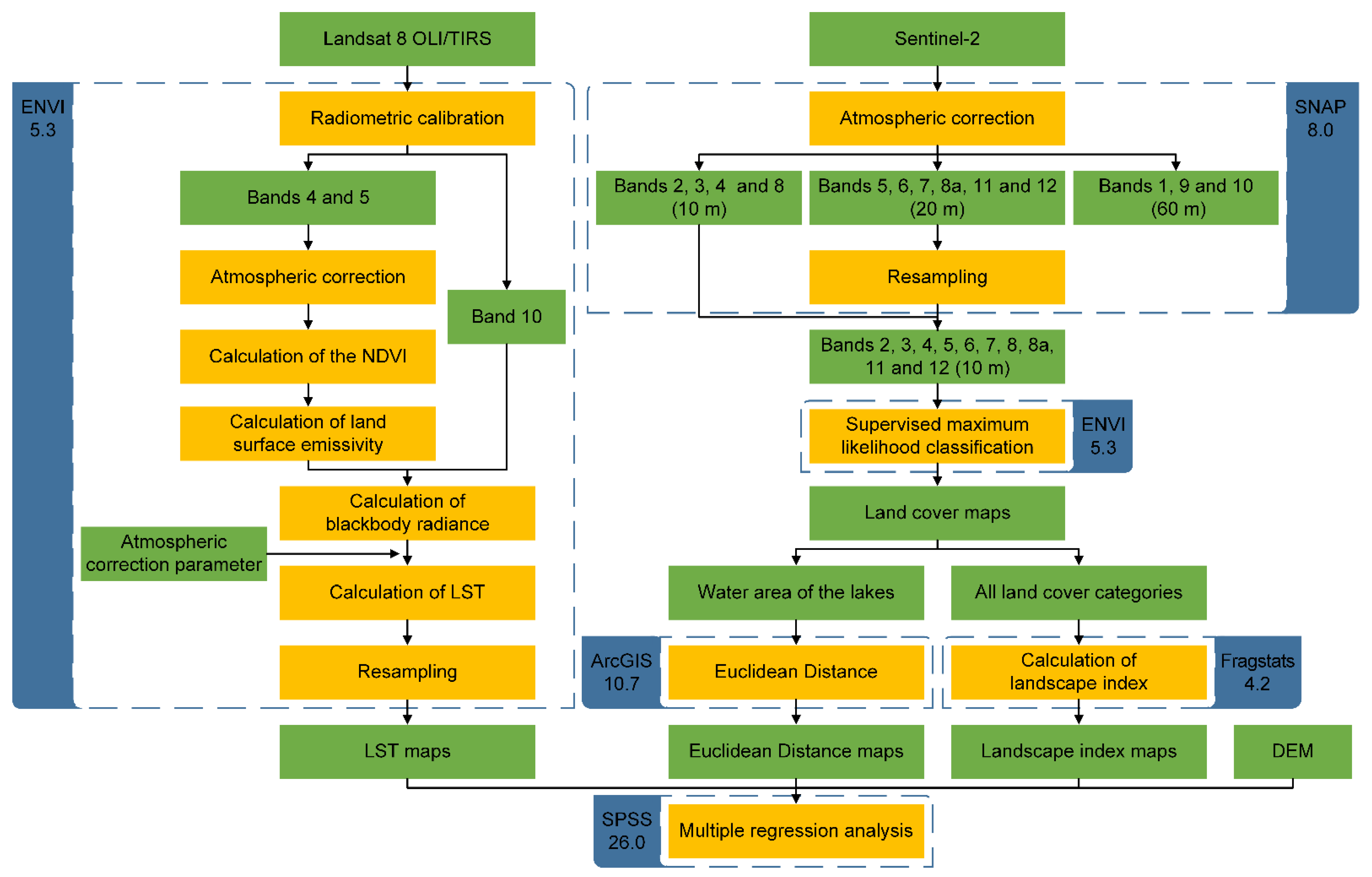
This study attempted to detect the cooling effects and scales of urban lakes using Landsat 8 OLI/TIRS and Sentinel-2 data. Herein, to accomplish this objective, the overall workflow was designed as follows (Figure 2), with four main procedures including: (1) LST inversion based on Landsat 8 OLI/TIRS images; (2) supervised maximum likelihood classification based on Sentinel-2 images; (3) landscape metrics measurement; and (4) multiple regression modeling of LST based on Euclidean distance maps, landscape composition and configuration indices, and digital elevation model (DEM).

2.4. LST Retrieval

The retrieval of LST followed the radiative transfer equation (RTE) method. The equation used to compute the thermal infrared radiance received by the sensor ( L λ ) is mentioned as given [42,43]:
L λ = [ ε B ( T S ) + ( 1 ε ) L a t m ] τ + L a t m
where ε is the land surface emissivity, B ( T S ) is the blackbody radiance (W/(m2∙sr∙μm)), T S is the LST (K), τ is atmospheric transmittance and L a t m and L a t m are upwelling and downwelling atmospheric radiance (W/(m2∙sr∙μm)), respectively. τ , L a t m and L a t m can be calculated on the Atmospheric Correction Parameter Calculator.
B ( T S ) is computed according to Equation (1). Subsequently, the LST is derived by Equation (2) [44]:
T S = K 2 ln ( K 1 B ( T S ) + 1 )
where K 1 is conversion constant 774.8853 W/(m2∙sr∙μm) and K 2 is conversion constant 1321.0789 K.
The land surface emissivity of water is 0.995, and the values of buildings and soil are obtained by the following equations [45]:
ε b u i l d i n g = 0.9589 + 0.0860 P v 0.0671 P v 2
ε s o i l = 0.9625 + 0.0614 P v 0.0461 P v 2
where P V is the vegetation proportion calculated by Equation (5) [46]:
P V = N D V I N D V I S o i l N D V I V e g N D V I S o i l
where NDVI is the normalized difference vegetation index, N D V I S o i l is the NDVI value of bare soil, N D V I V e g is the NDVI value of the area completely covered by vegetation. The equation of NDVI is [47]:
N D V I = ρ N I R ρ R e d ρ N I R + ρ R e d
where ρ N I R refers to the surface reflectance of NIR band (band 5, 0.845 0.885   μ m ), ρ R e d refers to the surface reflectance of Red band (band 4, 0.630 0.680   μ m ).
In addition, the LST data was up-sampled to 10 m resolution by nearest-neighbor interpolation to match the spatial resolution of Sentinel-2 data.

2.5. Land Cover Classification

The land cover classification was derived from the pre-processed Sentinel-2 images using the maximum likelihood supervised classification method. The land cover classification system developed by Cadenasso et al. [48] was adopted to classify the land cover into five categories, namely coarse-textured vegetation (CV), fine-textured vegetation (FV), impervious surface (IS), bare lands (BL), and water. The detailed information of these categories is shown in Table 2. The accuracy of classification was evaluated using 500 random points located in each classified land-cover map with reference to the ground-truth data in Google Earth. The results showed that the overall accuracies [49] of the classifications were 91.20% for Hangzhou and 91.67% for Nanjing. The kappa coefficients were 0.878 for Hangzhou and 0.883 for Nanjing.

2.6. Landscape Metrics-Based Analysis

Numerous landscape metrics have arisen as a method to quantify landscape patterns [50]. Herein, five commonly used class-level landscape metrics [51,52,53,54] were employed to relate the spatial variability of LST with the landscape patterns, including one composition metric: percentage of landscape (PLAND), and four configuration metrics: (1) Largest patch index (LPI); (2) Mean shape index (SHAPE_MN); (3) Aggregation index (AI); and (4) Patch density (PD) (Table 3). These metrics were selected according to the following principles [55,56]: (1) importance in both theory and practice; (2) simplicity in both calculation and interpretation; and (3) minimal redundancy. Fragstats Version 4.2.1 was employed to calculate the selected metrics. The uniform tiles method was adopted to subdivide the landscape into square tiles representing sub-landscapes. Bartesaghi-Koc et al. [57] proposed that a 50 m × 50 m grid size is proper for local-scale studies if very-high resolution data are available. In comparison, studies employing data with coarser spatial resolutions (>10 m) may require larger grid resolutions (>100 m). Masoudi et al. [58] and Masoudi and Tan [59] recommended an optimal grid size of 240 × 240 m to explore the relationship between LST and the spatial pattern of urban green spaces. Herein, considering that the resolutions of LST and land cover maps are 10 m, the side length was chosen as integer multiples of 100 m (10 × 10 pixels).

2.7. Statistical Analysis

The scatter diagram has been widely employed for qualitatively discussing the relationships between LST and the distance to the water bodies in previous studies [33,61]. In addition, the affecting scale was acquired by seeking the stationary point of the fitting function of the scatter diagram [4].
Relationships between LST and multiple influencing factors (i.e., the distance to the lakes, landscape metrics, and elevation) were quantitatively examined through the multiple linear regression (MLR) (Equation (7)) [62].
Y = β 0 + i = 1 n β i X i + ε
where n is the number of the independent variable, β 0 is the intercept, β i is the regression coefficient for X i , and ε is the error term of the model.
To reduce the redundancy, a stepwise regression approach was adopted to identify closely linked variables with LST from the MLR models and provide their predictive importance for LST [6]. The significance levels at 0.05 and 0.1 were adopted as thresholds for adding and removing predictor variables, respectively. Additionally, in order to get more stable predictions, the variance inflation factor (VIF) was employed to detect multicollinearity. A VIF value equal to or larger than ten means near collinearity [63], indicating that the corresponding variables should be excluded. The remaining variables were analyzed again by the above-mentioned regression analysis until the absence of multicollinearity amongst selected variables.
We took 100 m as the step length and gradually added samples according to the distance to the lake, which was defined as the nearest distance to the lake shoreline. In other words, as the distance to the lake increased by 100 m, the samples covered by a certain distance were added to the existing samples. The process continued until the distance to the lake was not considered an independent variable of the stepwise regression model, indicating the influence of the target lakes on LST can be neglected. Each variable was pre-processed using the normalization method (Equation (8)) before the regression analysis [64].
X ^ i = X i X m i n X m a x X m i n
where X i , X m i n , and X m a x are the original, minimum, maximum value of a variable, respectively. The regression analyses were carried out with the Statistical Package for the Social Sciences (SPSS) Version 26.

3. Results

3.1. Spatial Distributions of Land Cover and LST

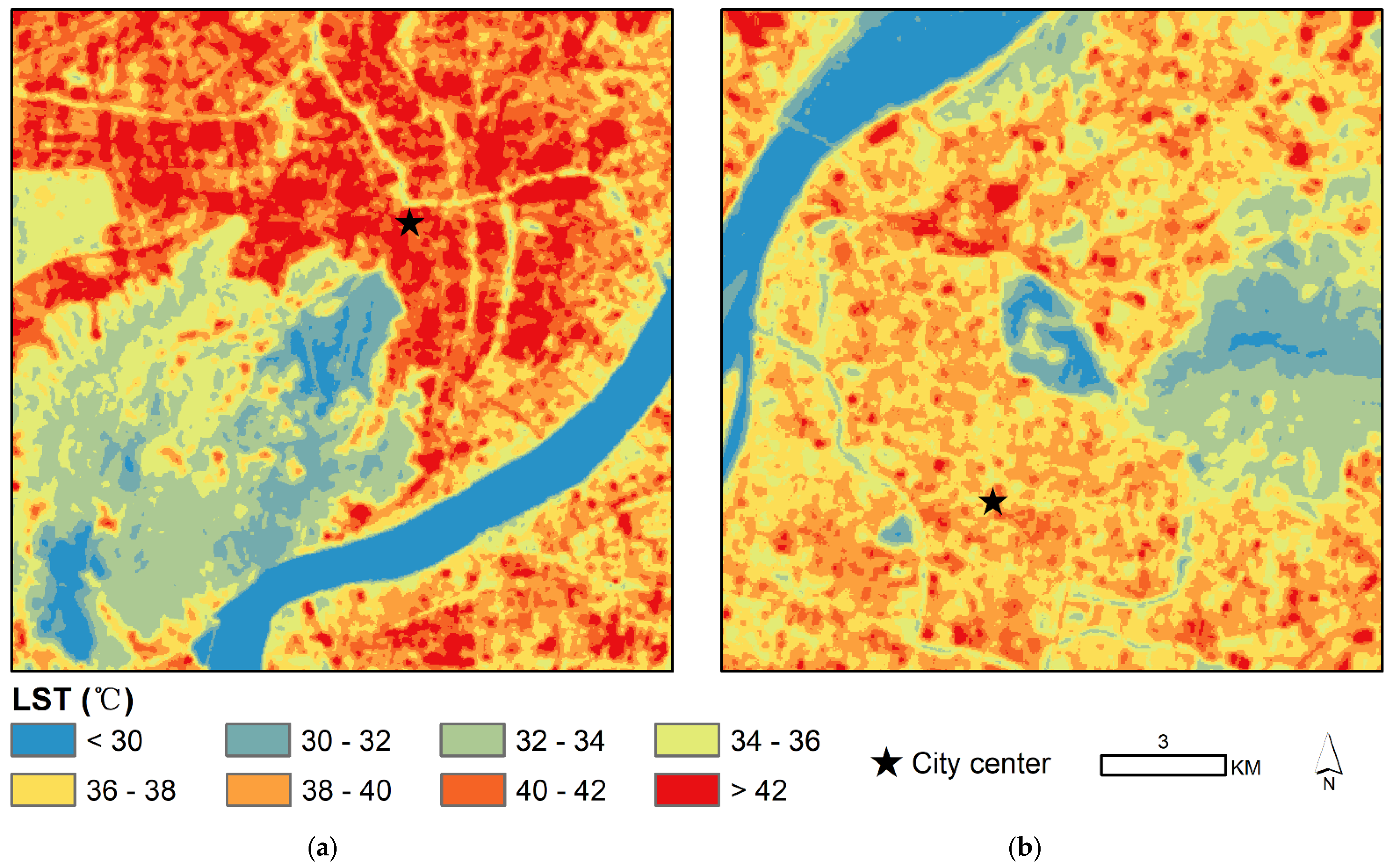
The spatial distribution of LST in Hangzhou and Nanjing were shown in Figure 3. The LST of Hangzhou ranged from 15.37 to 57.96 °C, with an average of 37.21 °C. The LST of Nanjing was between 28.28 and 50.72 °C, with an average of 36.45 °C. Temperature variation over impervious surface tended to be more variable, while the water-covered surface showed the opposite trend due to its high heat capacity. In Hangzhou, the north and east side of West Lake, mainly occupied by built-up areas, owned the highest LST. On the other hand, the south and west parts, dominated by CV, had lower LST. In addition, the Qiantang River passed through the southeast of the study area showing the lowest LST. For the case of Nanjing, Xuanwu Lake and the adjacent Zijin Mountain were the low-value areas of LST. The Yangtze River in the northwest of the study area owned the lowest LST, while the urban areas dominated by buildings had the highest LST.
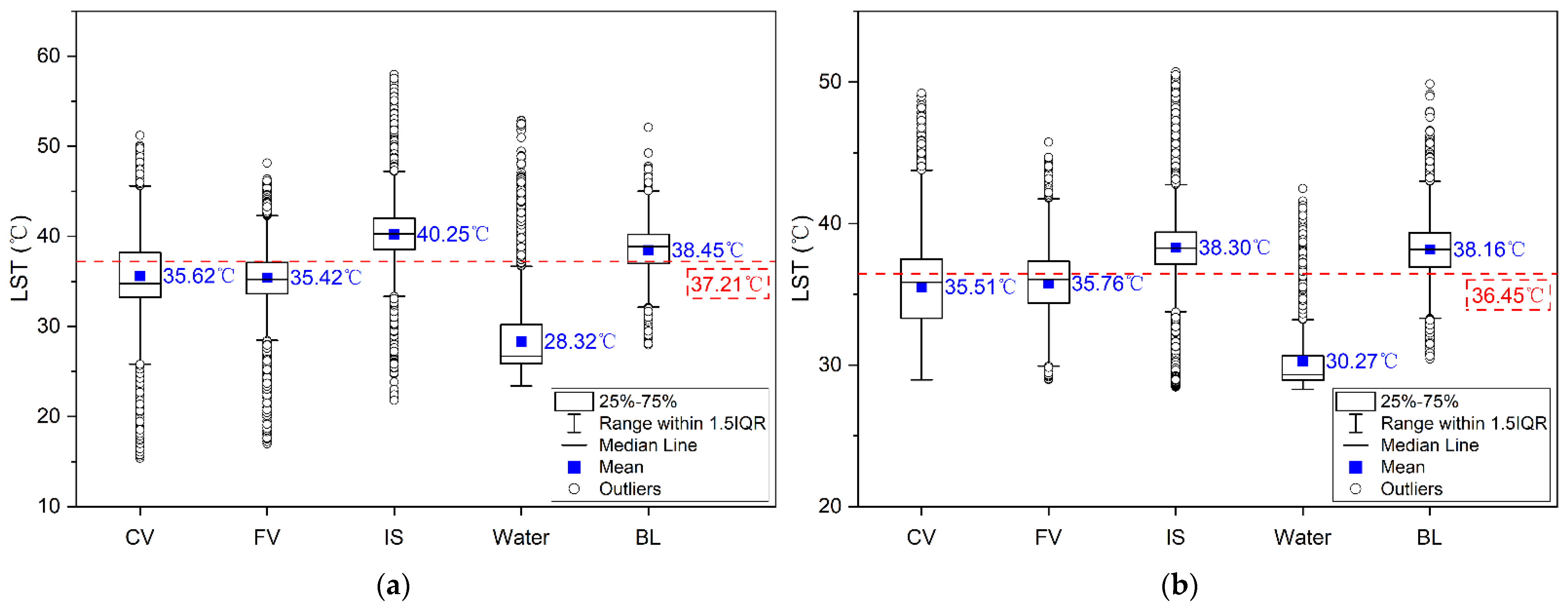
Similar LST patterns were observed in Hangzhou and Nanjing despite the different temperature conditions of the cities (Figure 4). The study areas were mainly covered by built-up areas, coarse-textured vegetation, and water body. The high-temperature region corresponding to the area was dominated by built-up, and the low-temperature region corresponding to the area were covered with water and coarse-textured vegetation. Compared with the average temperature (37.21 °C for Hangzhou and 36.45 °C for Nanjing), impervious surface (40.25 °C for Hangzhou and 38.30 °C for Nanjing) and bare land (38.45 °C for Hangzhou and 38.16 °C for Nanjing) had higher LST (Figure 5). In contrast, the LST of coarse-textured vegetation (35.62 °C for Hangzhou and 35.51 °C for Nanjing), fine-textured vegetation (35.42 °C for Hangzhou and 35.76 °C for Nanjing), and water (28.32 °C for Hangzhou and 30.27 °C for Nanjing) fell below the average line (Figure 5).

3.2. Drivers of LST Variations in the Lakes and Their Surrounding Areas

The results of the scatter diagrams showed an increasing trend of LST in response to the increase in distance to the lake within a certain scale (741 m for West Lake and 336 m for Xuanwu Lake) (Figure 6). The maximum cooling effects for West Lake and Xuanwu Lake were 4.86 °C and 4.78 °C, respectively. Additionally, the correlation analysis showed significant positive correlations between mean LST and the distance to the lake inside a certain scale. The Pearson correlation coefficients were 0.637 (p < 0.01) for West Lake, and 0.841 (p < 0.01) for Xuanwu Lake, respectively (Figure 6).
The scatter diagrams showed the relationships between LST and the distance to the water bodies intuitively but not quantitatively. Based on the above-mentioned affecting scale, multiple linear regression models were established to present the relationships quantitatively, and the significance tests were listed in Table 4 and Table 5. The models for Hangzhou (R2 > 0.81) and Nanjing (R2 > 0.65) were all of desirable goodness-of-fit.
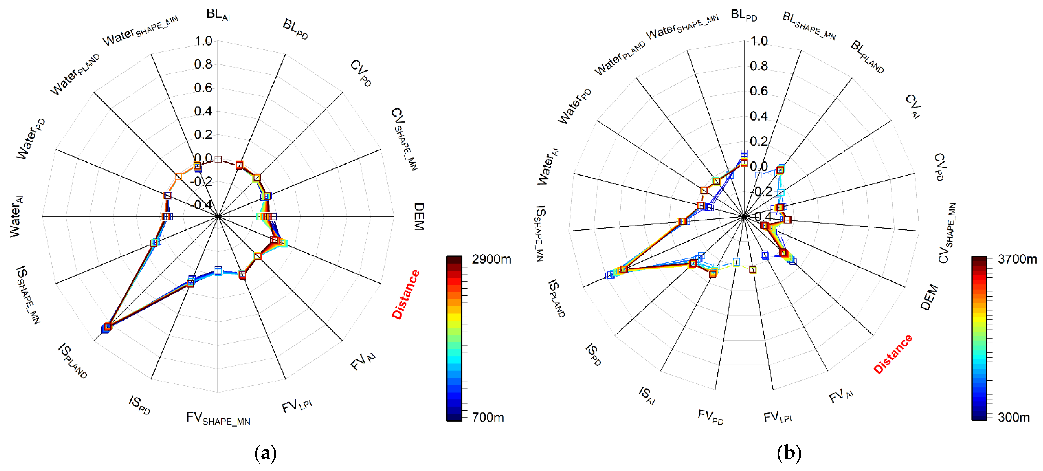
The multiple linear regressions showed that the distance to West Lake had significantly positive effects on LST in the range of 2900 m at the 5% significance level (Table 4 and Figure 7a). The distance to the Xuanwu Lake was a significant influencing factor in the range of 3700 m at the 5% significance level (Table 5 and Figure 7b).
As expected, the distance to the lake in both cities was positively related to LST regardless of the scale (Figure 7, Tables S1 and S2). Moreover, it is quite observant that as we examined LSTs at increasingly larger spatial extents, the standardized coefficients of distance generally had a decreasing trend, indicating that the explanatory power of distance parameters declined. The coefficients fluctuated between 0.078 and 0.110 in the first 1400 m around West Lake and kept decreasing in the extent of 1400 to 2900 m. For the Xuanwu Lake, the coefficients varied from 0.064 to 0.132 in the first 1200 m from the shoreline and showed a decreasing trend when the distance from the lake was more than 1200 m.
Although results from the MLRs showed that the distance to the lakes is an essential predictor of LST, the spatial configuration of impervious surface has a more significant effect on LST. The coefficients of the PLAND of IS were maintained at a high level both for West Lake (range from 0.811 to 0.867) and Xuanwu Lake (range from 0.639 to 0.779). In addition, with the decrease of the coefficients of distance, the coefficients of SHAPE_MN of IS showed higher values and tended to be stable after a certain distance (1800 m for West Lake and 1400 m for Xuanwu Lake). The coefficient values of PD of IS were steadily higher than that of distance after a certain distance (1500 m for West Lake and 1200 m for Xuanwu Lake). After 1500 m from Xuanwu Lake, the AI of IS also showed the same trend. The CV’s coefficients of SHAPE_MN (range from −0.077 to −0.036 for West Lake and −0.121 to −0.048 for Xuanwu Lake), PD (range from −0.051 to −0.027 for West Lake and −0.153 to −0.076 for Xuanwu Lake), and AI in Xuanwu Lake (range from −0.086 to −0.047) were negative regardless of the scale. DEM was negatively related to LST, and its coefficients varied greatly in the model with different scales. With the expansion of the spatial extent, the coefficients of DEM decreased first and then increased, and bottomed out at −0.150 in the model with a spatial extent of 1500 m for West Lake. On the scale of 600 m around Xuanwu Lake, DEM was not selected as the models’ variable, indicating that topography was not the main factor affecting LST. The first five models (600 m to 1100 m) that considered DEM as a dependent variable saw a dramatic fall in the coefficients of DEM, to a low of −0.204 in the model of 1100 m. Moreover, the coefficients of DEM dwindled to −0.231, after the rise to −0.152 in the extent of 1100 m to 3700 m.

4. Discussion

West Lake and Xuanwu Lake, located in the central areas of Hangzhou and Nanjing, showed a significant reduction of the LST in the surrounding areas up to a certain distance (741 m for West Lake and 336 m for Xuanwu Lake), demonstrating the ability of urban lakes in cooling the environment. Within the scale, the maximum cooling effects for West Lake and Xuanwu Lake were 4.86 and 4.78 °C, respectively. The cooling effect occurs when the thermal energy absorbed by the water is converted from sensible heating to latent heating with the production of water vapor [61]. Moreover, due to the high thermal capacity, the lakes own a lower temperature than the impervious surface during the daytime, which provides a higher pressure gradient for convective heat transfer [65]. Horizontal cooler air is generated above the lake and transported to the neighboring environment by the wind. The intensity of the processes decreases with the increasing distance to the lake, leading to the limited influence of the lakes on LST.
The ability of water bodies to adjust surrounding temperatures is determined both by the distance and its interactions with the surrounding environment [31]. However, most of the studies one-sidedly considered the distance to the water bodies, with little discussion on the integrated dynamics between the two features. Moyer and Hawkins [12] assessed the cooling effect of a fairly large river using urban temperature sensors deployed near the river. They reported that the UHI decreased by 0.6 °C to 0.3 °C for every 1000 m increase in distance from the river, depending on the season. Wu and Zhang [25] revealed that the horizontal cooling distance of Suzhou Bay could reach 800 m, and the maximum cooling effect was 3.02 °C. Cheval et al. [66] detected that the temperature regularly increases with the distance from the lake shoreline. Compared with these studies, our work underscored the necessity of considering the influence of its surrounding landscape patterns when quantifying the effects of the distance to the lakes on LST. In fact, most of the studies only focused on the scatter diagrams of LST to determine the cooling scale [4,33,61]. In contrast, after confirming the turning point from scatter diagrams, we continuously conducted a step-by-step multiple linear regression to detect the cooling potential of the two lakes on a much larger scale. The affecting scale obtained by seeking the stationary point of the fitting function of the scatter diagram was considered to be the region where the urban lakes massively lower the LST. The scale obtained by the multiple linear regression considering the influence of landscape patterns was deemed as the region where the urban lakes showed a significant capacity in cooling the environment. Although this study is conducted for West Lake and Xuanwu Lake, the general analysis procedure is flexible and can be extended to the case studies of urban lakes in other cities.
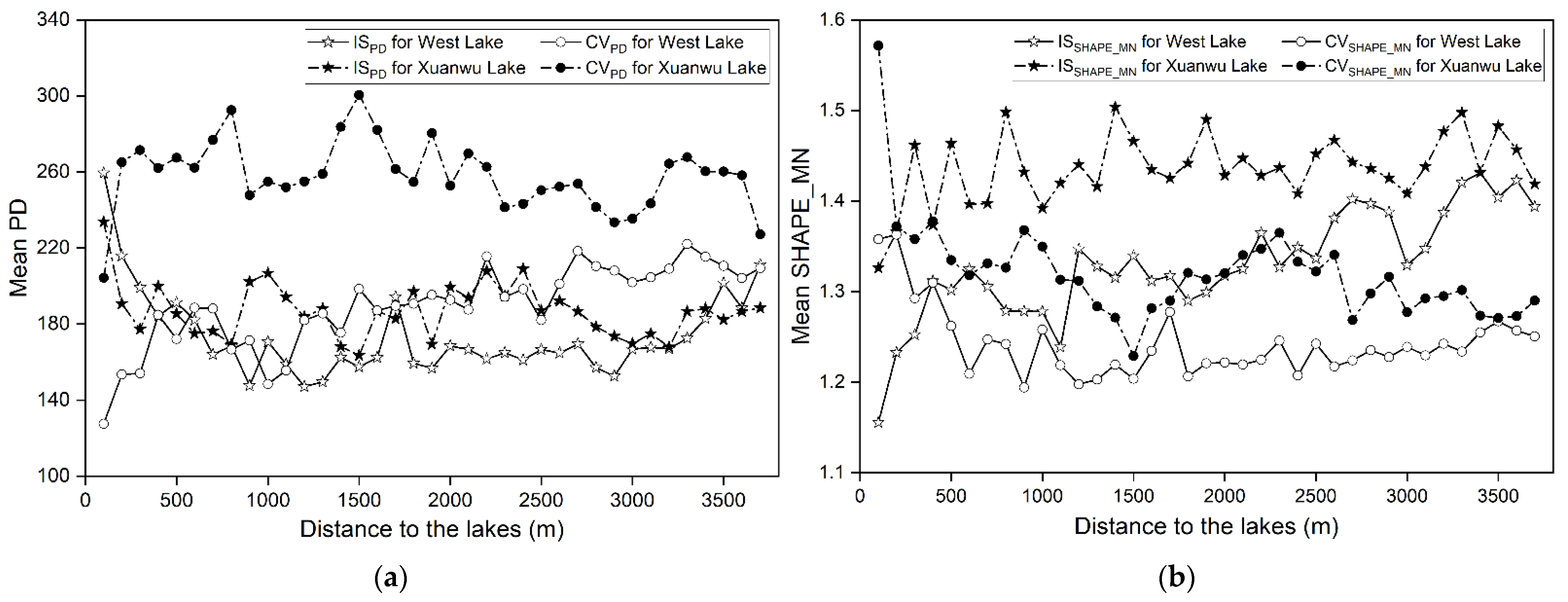
The regression results showed that although Xuanwu Lake was smaller in size, the maximum cooling scale could reach 3700 m, which was much larger than West Lake (2900 m). The cooling effect difference results from the surrounding landscape patterns, topography, and wind conditions (including wind directions and wind speed). It is demonstrated in Figure 8 that the PD of CV and the SHAPE_MN of IS around Xuanwu Lake were obviously higher than those of West Lake. High-density of trees and shrubs around the lake was conducive to forming a solid local circulation. The small and scattered architectural composition was instrumental in the formation of effective urban ventilation corridors [67], resulting in the expansion of the cooling range. In addition, large and dense buildings lead to significant heat effects [68,69]. To maximize the cooling potential of urban lakes, urban planners are suggested to arrange more trees and shrubs in the area around the lake and control the concentration of buildings. Meanwhile, West Lake is neighbored by mountains and is strongly impacted by a mountain valley breeze. Hence, the valley breeze in the northeast direction prevails in West Lake during the day [70], leading to the limited cooling effect on the urban area on the east side. Xuanwu Lake is mainly affected by east and southeast winds [71], which helps transport cooler air from the lake surface to the urban area.
Furthermore, as a famous tourist spot, West Lake, which ranked No.1 in the 2018 China National Scenic Spot Popularity Index Ranking, received 833,700 tourists only one day on 3 October 2018 [72]. The overloaded West Lake tourism was also considered a contribution to the emergence of heat islands in West Lake and its neighboring areas. Previous studies have shown the significant cooling effects of urban greenspace on LST [73,74,75]. Nonetheless, the PLAND of CV, which corresponds closely to the LST [76,77,78], was not considered as a predictor variable in the linear regression models. This is because a large number of samples in the study were composed of residential buildings and the greening around the buildings, resulting in a significant negative correlation between the PLAND of IS and CV (r = −0.738 and −0.670 in Hangzhou and Nanjing, respectively, p < 0.01). The VIF values of partial variables were much more significant than 10 when the PLAND of IS and CV were both considered as independent variables, indicating the existence of multicollinearity. In order to get satisfactory results in model accuracy and applicability, the problem of multicollinearity was eliminated by excluding the factor, the PLAND of CV.
Several limitations of this work should be addressed for future research avenues. First, the influence of the inherent properties of lakes (e.g., the size, shape, and water volume) on their cooling effect is not considered due to the limited number of lakes. Moreover, it is found that the relationship between landscape metrics and LST varies with the change of grid size. In this context, multi-scale analysis is needed in further studies to explore the cooling effects of urban lakes fully. Finally, this study was conducted in two cities with similar climatic conditions. The results may differ for other cities with a different climate. Thus, future studies involving other urban lakes with different climatic conditions are expected.

5. Conclusions

This study applied a distance—LST scatter diagram and multiple linear regression method to detect the cooling effect and scale of urban lakes based on Landsat 8 OLI/TIRS and Sentinel-2 data. Taking two famous city inner lakes, West Lake and Xuanwu Lake, as the study sites, the cooling effect and the potential cooling scale of large inner-city lakes were quantitatively analyzed. Meanwhile, the landscape patterns in the surrounding areas of the urban lake were considered as independent variables to detect the relationship in different scales. The whole research flow provides a complete procedure to detect the maximum cooling distance of a large cooling resource and can be applied not only to lakes but also to other specific complete cooling resources such as a park, a river, and a wetland. The results show that West Lake and Xuanwu Lake massively reduced the land surface temperature of surrounding areas within a certain distance (471 m for West Lake and 336 m for Xuanwu Lake) and had potential cooling effects on a larger scale (2900 m for West Lake and 3700 m for Xuanwu Lake). The results proved that the turning point in the temperature diagram could not reflect the cooling scale, and the exact cooling scale could be much larger. In addition, from the comparative study between Hangzhou and Nanjing, we detect the phenomenon that the surrounding landscape composition and configuration could strongly affect the maximum cooling scale. In detail, the high density of trees and shrubs, together with small and scattered buildings, could contribute to the extension of the cooling scale of inner lakes. However, to completely show the influencing factors for the cooling intensity and scale, future studies are suggested to consider more samples and consider the size and shape of lakes. In general, this research expands our scientific understanding of urban lakes’ cooling effects, especially the potential cooling scale. These findings provide insights for urban planners to arrange the landscape of surrounding areas of large inner-city lakes to pursuit better environmental outcomes.

Supplementary Materials

The following are available online at https://www.mdpi.com/article/10.3390/rs13081526/s1, Table S1: The coefficients of the multiple linear stepwise regression models at different scales for the West Lake. The bold and italic rows are standardized coefficients, Table S2: The coefficients of the multiple linear stepwise regression models at different scales for Xuanwu Lake. The bold and italic rows are standardized coefficients.

Author Contributions

Conceptualization, Y.Z., Y.L., and H.H.; methodology, Y.Z. and H.H.; software, Y.Z.; formal analysis, Y.Z. and H.H.; investigation, Y.Z., Y.L., and H.H.; resources, Y.Z.; data curation, Y.Z.; writing—original draft preparation, Y.Z. and Y.L.; writing—review and editing, H.H., Y.M., R.W., and T.H.; visualization, Y.Z.; supervision, H.H.; project administration, H.H.; funding acquisition, H.H and R.W. All authors have read and agreed to the published version of the manuscript.

Funding

This research was supported by the Natural Science Foundation of Zhejiang Province: LQ20D010008 (Representative: Hao Hou), and the Japan Society for the Promotion of Science (JSPS) Doctoral Fellowship: 19J11409 (Representative: Ruci Wang).

Institutional Review Board Statement

Not applicable.

Informed Consent Statement

Not applicable.

Data Availability Statement

The data that support the findings of this study are available from the author upon reasonable request.

Acknowledgments

The authors appreciate the editors and anonymous reviewers for their valuable comments and suggestions.

Conflicts of Interest

The authors declare no conflict of interest.

References

  1. Grimm, N.B.; Faeth, S.H.; Golubiewski, N.E.; Redman, C.L.; Wu, J.; Bai, X.; Briggs, J.M. Global change and the ecology of cities. Science 2008, 319, 756–760. [Google Scholar] [CrossRef] [PubMed] [Green Version]
  2. Pascual, J.I.; Lorente, N.; Song, Z.; Conrad, H.; Rust, H.P. Selectivity in vibrationally mediated single-molecule chemistry. Nature 2003, 423, 525–528. [Google Scholar] [CrossRef]
  3. Howard, L. The Climate of London; London Harvey and Dorton: London, UK, 1833; Volume 2, pp. 1818–1820. [Google Scholar]
  4. Hou, H.; Estoque, R.C. Detecting Cooling Effect of Landscape from Composition and Configuration: An Urban Heat Island Study on Hangzhou. Urban For. Urban Green. 2020, 53, 126719. [Google Scholar] [CrossRef]
  5. Ganeshan, M.; Murtugudde, R.; Imhoff, M.L. A multi-city analysis of the UHI-influence on warm season rainfall. Urban Clim. 2013, 6, 1–23. [Google Scholar] [CrossRef]
  6. Zhou, W.; Huang, G.; Cadenasso, M.L. Does spatial configuration matter? Understanding the effects of land cover pattern on land surface temperature in urban landscapes. Landsc. Urban Plan. 2011, 102, 54–63. [Google Scholar] [CrossRef]
  7. Santamouris, M.; Cartalis, C.; Synnefa, A.; Kolokotsa, D. On the impact of urban heat island and global warming on the power demand and electricity consumption of buildings—A review. Energy Build. 2015, 98, 119–124. [Google Scholar] [CrossRef]
  8. Rocklöv, J.; Forsberg, B.; Ebi, K.; Bellander, T. Susceptibility to mortality related to temperature and heat and cold wave duration in the population of Stockholm County, Sweden. Glob. Health Action 2014, 7, 22737. [Google Scholar] [CrossRef] [Green Version]
  9. Wong, L.P.; Alias, H.; Aghamohammadi, N.; Aghazadeh, S.; Sulaiman, N.M.N. Urban heat island experience, control measures and health impact: A survey among working community in the city of Kuala Lumpur. Sustain. Cities Soc. 2017, 35, 660–668. [Google Scholar] [CrossRef]
  10. Wu, Y.; Zhang, M.; Hong, L.; Xian, X.; Yang, K. Temporal and Spatial Variation of Urban Heat Island Effect in Plateau Lake Region Based on RS—A 30-Year Case Study in Dianchi Basin. In Proceedings of the 2018 26th International Conference on Geoinformatics, Kunming, China, 28–30 June 2018; pp. 1–6. [Google Scholar]
  11. Hathway, E.A.; Sharples, S. The interaction of rivers and urban form in mitigating the Urban Heat Island effect: A UK case study. Build. Environ. 2012, 58, 14–22. [Google Scholar] [CrossRef] [Green Version]
  12. Moyer, A.N.; Hawkins, T.W. River effects on the heat island of a small urban area. Urban Clim. 2017, 21, 262–277. [Google Scholar] [CrossRef]
  13. Voogt, J.A.; Oke, T.R. Thermal remote sensing of urban climates. Remote Sens. Environ. 2003, 86, 370–384. [Google Scholar] [CrossRef]
  14. Hu, L.; Sun, Y.; Collins, G.; Fu, P. Improved estimates of monthly land surface temperature from MODIS using a diurnal temperature cycle (DTC) model. ISPRS J. Photogramm. Remote Sens. 2020, 168, 131–140. [Google Scholar] [CrossRef]
  15. Chen, L.; Wang, X.; Cai, X.; Yang, C.; Lu, X. Seasonal Variations of Daytime Land Surface Temperature and Their Underlying Drivers over Wuhan, China. Remote Sens. 2021, 13, 323. [Google Scholar] [CrossRef]
  16. Cao, H.; Gao, B.; Gong, T.; Wang, B. Analyzing Changes in Frozen Soil in the Source Region of the Yellow River Using the MODIS Land Surface Temperature Products. Remote Sens. 2021, 13, 180. [Google Scholar] [CrossRef]
  17. Ngie, A.; Abutaleb, K.; Ahmed, F.; Darwish, A.; Ahmed, M. Assessment of urban heat island using satellite remotely sensed imagery: A review. S. Afr. Geogr. J. 2014, 96, 198–214. [Google Scholar] [CrossRef]
  18. Zhou, D.; Zhao, S.; Liu, S.; Zhang, L.; Zhu, C. Surface urban heat island in China’s 32 major cities: Spatial patterns and drivers. Remote Sens. Environ. 2014, 152, 51–61. [Google Scholar] [CrossRef]
  19. Clinton, N.; Gong, P. MODIS detected surface urban heat islands and sinks: Global locations and controls. Remote Sens. Environ. 2013, 134, 294–304. [Google Scholar] [CrossRef]
  20. Khorchani, M.; Vicente-Serrano, S.M.; Azorin-Molina, C.; Garcia, M.; Martin-Hernandez, N.; Peña-Gallardo, M.; Kenawy, A.E.; Domínguez-Castro, F. Trends in LST over the peninsular Spain as derived from the AVHRR imagery data. Global Planet. Chang. 2018, 166, 75–93. [Google Scholar] [CrossRef]
  21. Chen, X.; Zhao, H.; Li, P.; Yin, Z. Remote sensing image-based analysis of the relationship between urban heat island and land use/cover changes. Remote Sens. Environ. 2006, 104, 133–146. [Google Scholar] [CrossRef]
  22. Zhao, L.; Lee, X.; Smith, R.B.; Oleson, K. Strong contributions of local background climate to urban heat islands. Nature 2014, 511, 216–219. [Google Scholar] [CrossRef]
  23. Streutker, D.R. Satellite-measured growth of the urban heat island of Houston, Texas. Remote Sens. Environ. 2003, 85, 282–289. [Google Scholar] [CrossRef]
  24. Wu, C.; Li, J.; Wang, C.; Song, C.; Chen, Y.; Finka, M.; Rosa, D.L. Understanding the relationship between urban blue infrastructure and land surface temperature. Sci. Total. Environ. 2019, 694, 133742. [Google Scholar] [CrossRef]
  25. Wu, Z.; Zhang, Y. Water Bodies’ Cooling Effects on Urban Land Daytime Surface Temperature: Ecosystem Service Reducing Heat Island Effect. Sustainability 2019, 11, 787. [Google Scholar] [CrossRef] [Green Version]
  26. Deilami, K.; Kamruzzaman, M.; Liu, Y. Urban heat island effect: A systematic review of spatio-temporal factors, data, methods, and mitigation measures. Int. J. Appl. Earth Obs. Geoinf. 2018, 67, 30–42. [Google Scholar] [CrossRef]
  27. Arnfield, A.J. Two decades of urban climate research: A review of turbulence, exchanges of energy and water, and the urban heat island. Int. J. Climatol. 2003, 23, 1–26. [Google Scholar] [CrossRef]
  28. Schwarz, N.; Manceur, A.M. Analyzing the Influence of Urban Forms on Surface Urban Heat Islands in Europe. J. Urban Plan. Dev. 2015, 141, A4014003. [Google Scholar] [CrossRef]
  29. Theeuwes, N.E.; Solcerová, A.; Steeneveld, G.J. Modeling the influence of open water surfaces on the summertime temperature and thermal comfort in the city. J. Geophys. Res.: Atmos. 2013, 118, 8881–8896. [Google Scholar] [CrossRef] [Green Version]
  30. Spronken-Smith, R.A.; Oke, T.R.; Lowry, W.P. Advection and the surface energy balance across an irrigated urban park. Int. J. Climatol. 2000, 20, 1033–1047. [Google Scholar] [CrossRef]
  31. Gunawardena, K.R.; Wells, M.J.; Kershaw, T. Utilising green and bluespace to mitigate urban heat island intensity. Sci. Total Environ. 2017, 584–585, 1040–1055. [Google Scholar] [CrossRef]
  32. Song, W.; Xu, Q.; Fu, X.; Zhang, P.; Pang, Y.; Song, D. Research on the Relationship between Water Diversion and Water Quality of Xuanwu Lake, China. Int. J. Environ. Res. Public Health 2018, 15, 1262. [Google Scholar] [CrossRef] [Green Version]
  33. Cai, Z.; Han, G.; Chen, M. Do water bodies play an important role in the relationship between urban form and land surface temperature? Sustain. Cities Soc. 2018, 39, 487–498. [Google Scholar] [CrossRef]
  34. Xu, S.; Liu, Y.; Qian, Y.; Wang, Q. The significance of the West Lake pattern and its heuristic implications for creating China’s heritage tourism economics. Tour. Manag. 2017, 58, 286–292. [Google Scholar] [CrossRef]
  35. Hangzhou Municipal Bureau of Statistics. An Overview of Hangzhou. Available online: http://tjj.hangzhou.gov.cn/ (accessed on 26 January 2021).
  36. Nanjing Municipal Bureau of Statistics. Nanjing Statistical Yearbook 2020. Available online: http://tjj.nanjing.gov.cn/material/njnj_2020/ (accessed on 26 January 2021).
  37. Wang, L.; Hou, H.; Weng, J. Ordinary least squares modelling of urban heat island intensity based on landscape composition and configuration: A comparative study among three megacities along the Yangtze River. Sustain. Cities Soc. 2020, 62, 102381. [Google Scholar] [CrossRef]
  38. Gascon, F.; Bouzinac, C.; Thépaut, O.; Jung, M.; Francesconi, B.; Louis, J.; Lonjou, V.; Lafrance, B.; Massera, S.; Gaudel-Vacaresse, A.; et al. Copernicus Sentinel-2A Calibration and Products Validation Status. Remote Sens. 2017, 9, 584. [Google Scholar] [CrossRef] [Green Version]
  39. Shao, Z.; Cai, J.; Fu, P.; Hu, L.; Liu, T. Deep learning-based fusion of Landsat-8 and Sentinel-2 images for a harmonized surface reflectance product. Remote Sens. Environ. 2019, 235, 111425. [Google Scholar] [CrossRef]
  40. Fernandez-Beltran, R.; Baidar, T.; Kang, J.; Pla, F. Rice-Yield Prediction with Multi-Temporal Sentinel-2 Data and 3D CNN: A Case Study in Nepal. Remote Sens. 2021, 13, 1391. [Google Scholar] [CrossRef]
  41. Persson, H.J.; Jonzén, J.; Nilsson, M. Combining TanDEM-X and Sentinel-2 for large-area species-wise prediction of forest biomass and volume. Int. J. Appl. Earth Obs. Geoinf. 2021, 96, 102275. [Google Scholar] [CrossRef]
  42. Sobrino, J.A.; Jiménez-Muñoz, J.C.; Paolini, L. Land surface temperature retrieval from LANDSAT TM 5. Remote Sens. Environ. 2004, 90, 434–440. [Google Scholar] [CrossRef]
  43. Windahl, E.; Beurs, K.d. An intercomparison of Landsat land surface temperature retrieval methods under variable atmospheric conditions using in situ skin temperature. Int. J. Appl. Earth Obs. Geoinf. 2016, 51, 11–27. [Google Scholar] [CrossRef] [Green Version]
  44. Chander, G.; Markham, B.L.; Helder, D.L. Summary of current radiometric calibration coefficients for Landsat MSS, TM, ETM+, and EO-1 ALI sensors. Remote Sens. Environ. 2009, 113, 893–903. [Google Scholar] [CrossRef]
  45. Qin, Z.; Li, W.; Xu, B.; Chen, Z.; Liu, J. The estimation of land surface emissivity for Landsat TM6. Remote Sens. Land Resour. 2004, 16, 28–32,36,41. [Google Scholar] [CrossRef]
  46. Carlson, T.N.; Ripley, D.A. On the relation between NDVI, fractional vegetation cover, and leaf area index. Remote Sens. Environ. 1997, 62, 241–252. [Google Scholar] [CrossRef]
  47. Becker, F.; Choudhury, B.J. Relative sensitivity of normalized difference vegetation Index (NDVI) and microwave polarization difference Index (MPDI) for vegetation and desertification monitoring. Remote Sens. Environ. 1988, 24, 297–311. [Google Scholar] [CrossRef]
  48. Cadenasso, M.L.; Pickett, S.T.A.; Schwarz, K. Spatial heterogeneity in urban ecosystems: Reconceptualizing land cover and a framework for classification. Front. Ecol. Environ. 2007, 5, 80–88. [Google Scholar] [CrossRef]
  49. Congalton, R.G. A review of assessing the accuracy of classifications of remotely sensed data. Remote Sens. Environ. 1991, 37, 35–46. [Google Scholar] [CrossRef]
  50. O’Neill, R.V.; Krummel, J.R.; Gardner, R.H.; Sugihara, G.; Jackson, B.; Deangelis, D.L.; Milne, B.T.; Turner, M.G.; Zygmunt, B.; Christensen, S.W.; et al. Indices of landscape pattern. Landsc. Ecol. 1988, 1, 153–162. [Google Scholar] [CrossRef]
  51. Chen, A.; Yao, L.; Sun, R.; Chen, L. How many metrics are required to identify the effects of the landscape pattern on land surface temperature? Ecol. Indic. 2014, 45, 424–433. [Google Scholar] [CrossRef]
  52. Estoque, R.C.; Murayama, Y.; Myint, S.W. Effects of landscape composition and pattern on land surface temperature: An urban heat island study in the megacities of Southeast Asia. Sci. Total Environ. 2017, 577, 349–359. [Google Scholar] [CrossRef]
  53. Yao, L.; Li, T.; Xu, M.; Xu, Y. How the landscape features of urban green space impact seasonal land surface temperatures at a city-block-scale: An urban heat island study in Beijing, China. Urban For. Urban Green. 2020, 52, 126704. [Google Scholar] [CrossRef]
  54. Zhou, W.; Cao, F. Effects of changing spatial extent on the relationship between urban forest patterns and land surface temperature. Ecol. Indic. 2020, 109, 105778. [Google Scholar] [CrossRef]
  55. Maimaitiyiming, M.; Ghulam, A.; Tiyip, T.; Pla, F.; Latorre-Carmona, P.; Halik, Ü.; Sawut, M.; Caetano, M. Effects of green space spatial pattern on land surface temperature: Implications for sustainable urban planning and climate change adaptation. ISPRS J. Photogramm. Remote Sens. 2014, 89, 59–66. [Google Scholar] [CrossRef] [Green Version]
  56. Zhou, W.; Wang, J.; Cadenasso, M.L. Effects of the spatial configuration of trees on urban heat mitigation: A comparative study. Remote Sens. Environ. 2017, 195, 1–12. [Google Scholar] [CrossRef]
  57. Bartesaghi-Koc, C.; Osmond, P.; Peters, A. Spatio-temporal patterns in green infrastructure as driver of land surface temperature variability: The case of Sydney. Int. J. Appl. Earth Obs. Geoinf. 2019, 83, 101903. [Google Scholar] [CrossRef]
  58. Masoudi, M.; Tan, P.Y.; Fadaei, M. The effects of land use on spatial pattern of urban green spaces and their cooling ability. Urban Clim. 2021, 35, 100743. [Google Scholar] [CrossRef]
  59. Masoudi, M.; Tan, P.Y. Multi-year comparison of the effects of spatial pattern of urban green spaces on urban land surface temperature. Landsc. Urban Plan. 2019, 184, 44–58. [Google Scholar] [CrossRef]
  60. McGarigal, K.; Cushman, S.A.; Neel, M.C.; Ene, E. FRAGSTATS: Spatial Pattern Analysis Program for Categorical Maps. Available online: http://www.umass.edu/landeco/research/fragstats/fragstats.html (accessed on 26 January 2021).
  61. Gupta, N.; Mathew, A.; Khandelwal, S. Analysis of cooling effect of water bodies on land surface temperature in nearby region: A case study of Ahmedabad and Chandigarh cities in India. Egypt. J. Remote Sens. Space Sci. 2019, 22, 81–93. [Google Scholar] [CrossRef]
  62. Pardoe, I. Multiple Linear Regression. In Applied Regression Modeling, 3rd ed.; Pardoe, I., Ed.; John Wiley & Sons, Inc: Hoboken, NJ, USA, 2020; Volume 3, pp. 96–100. [Google Scholar]
  63. Franklin, J.B.; Sathish, T.; Vinithkumar, N.V.; Kirubagaran, R. A novel approach to predict chlorophyll-a in coastal-marine ecosystems using multiple linear regression and principal component scores. Mar. Pollut. Bull. 2020, 152, 110902. [Google Scholar] [CrossRef]
  64. Yuan, D.; Elvidge, C.D. Comparison of relative radiometric normalization techniques. ISPRS J. Photogramm. Remote Sens. 1996, 51, 117–126. [Google Scholar] [CrossRef]
  65. Sun, R.; Chen, L. How can urban water bodies be designed for climate adaptation? Lands. Urban Plan. 2012, 105, 27–33. [Google Scholar] [CrossRef]
  66. Cheval, S.; Popa, A.-M.; Șandric, I.; Iojă, I.-C. Exploratory analysis of cooling effect of urban lakes on land surface temperature in Bucharest (Romania) using Landsat imagery. Urban. Clim. 2020, 34, 100696. [Google Scholar] [CrossRef]
  67. Zhang, Q.; Wen, Y.; Wu, Z.; Chen, Y. Seasonal Variations of the Cooling Effect of Water Landscape in High-density Urban Built-up Area: A Case Study of the Center Urban District of Guangzhou. Ecol. Environ. Sci. 2018, 27, 1323–1334. [Google Scholar] [CrossRef]
  68. Athukorala, D.; Murayama, Y. Spatial Variation of Land Use/Cover Composition and Impact on Surface Urban Heat Island in a Tropical Sub-Saharan City of Accra, Ghana. Sustainability 2020, 12, 7953. [Google Scholar] [CrossRef]
  69. Liu, F.; Hou, H.; Murayama, Y. Spatial Interconnections of Land Surface Temperatures with Land Cover/Use: A Case Study of Tokyo. Remote Sens. 2021, 13, 610. [Google Scholar] [CrossRef]
  70. Yu, B.; He, X.; Wei, L.; Chen, L.; Zhou, W. Primary exploration for construction of urban multilevel ventilation corridors system in Hangzhou. J. Meteorol. Sci. 2018, 38, 625–636. [Google Scholar] [CrossRef]
  71. Zhang, Y.; Rui, D.; Zhou, L. Nanjing Zhongshan Mountain Scenic’s Influence on the Air Quality in Main Urban Area. Environ. Monit. Forewarning 2010, 2, 47–50. [Google Scholar] [CrossRef]
  72. Fei, J.; Chen, W.; Bao, Q.; Zhang, W. Evolution Characteristics and Multi-Value of Scenic Byway of the West Lake Mountain Forest in Hangzhou. J. Chin. Urban For. 2020, 18, 98–102. [Google Scholar] [CrossRef]
  73. Jenerette, G.D.; Harlan, S.L.; Brazel, A.; Jones, N.; Larsen, L.; Stefanov, W.L. Regional relationships between surface temperature, vegetation, and human settlement in a rapidly urbanizing ecosystem. Lands. Ecol. 2007, 22, 353–365. [Google Scholar] [CrossRef]
  74. Soydan, O. Effects of landscape composition and patterns on land surface temperature: Urban heat island case study for Nigde, Turkey. Urban. Clim. 2020, 34, 100688. [Google Scholar] [CrossRef]
  75. Liu, Y.; Huang, X.; Yang, Q.; Cao, Y. The turning point between urban vegetation and artificial surfaces for their competitive effect on land surface temperature. J.Clean. Prod. 2021, 292, 126034. [Google Scholar] [CrossRef]
  76. Kong, F.; Yin, H.; James, P.; Hutyra, L.R.; He, H.S. Effects of spatial pattern of greenspace on urban cooling in a large metropolitan area of eastern China. Lands. Urban Plan. 2014, 128, 35–47. [Google Scholar] [CrossRef]
  77. Fan, H.; Yu, Z.; Yang, G.; Liu, T.Y.; Liu, T.Y.; Hung, C.H.; Vejre, H. How to cool hot-humid (Asian) cities with urban trees? An optimal landscape size perspective. Agric. For. Meteorol. 2019, 265, 338–348. [Google Scholar] [CrossRef]
  78. Wang, R.; Hou, H.; Murayama, Y.; Derdouri, A. Spatiotemporal Analysis of Land Use/Cover Patterns and Their Relationship with Land Surface Temperature in Nanjing, China. Remote Sens. 2020, 12, 440. [Google Scholar] [CrossRef] [Green Version]
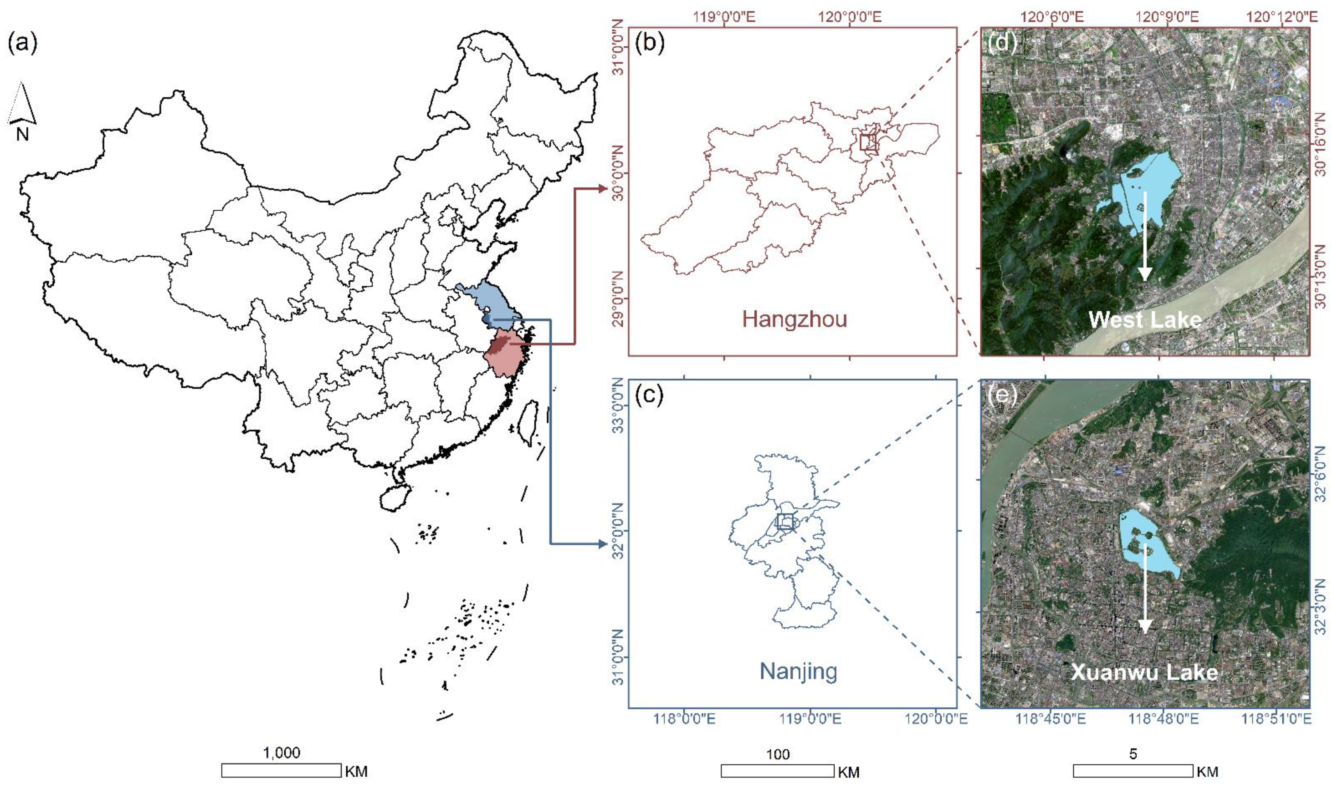
Figure 1. Location of the study area. (a) Map of China; (b) map of Hangzhou; (c) map of Nanjing; (d) Sentinel-2 image of West Lake and its neighboring areas; and (e) Sentinel-2 image of Xuanwu Lake and its neighboring areas. The sentinel-2 images were displayed in true color composite (Red—Band 4; Green—Band 3; and Bule—Band 2).
Remotesensing 13 01526 g001
Figure 2. Overall workflow of this study. Green, yellow, and blue represent data, operations, and software, respectively.
Remotesensing 13 01526 g002
Figure 3. The land surface temperature (LST) maps of (a) West Lake and its neighboring areas in Hangzhou, and (b) Xuanwu Lake and its neighboring areas in Nanjing.
Remotesensing 13 01526 g003
Figure 4. The land cover maps of (a) West Lake and its neighboring areas in Hangzhou, and (b) Xuanwu Lake and its neighboring areas in Nanjing (CV: coarse-textured vegetation; FV: fine-textured vegetation; IS: impervious surface; BL: bare lands; Water: water).
Remotesensing 13 01526 g004
Figure 5. LST of land cover categories in (a) West Lake and its neighboring areas in Hangzhou, and (b) Xuanwu Lake and its neighboring areas in Nanjing (CV: coarse-textured vegetation; FV: fine-textured vegetation; IS: impervious surface; BL: bare lands; Water: water).
Remotesensing 13 01526 g005
Figure 6. Mean LST at different distances to (a) West Lake in Hangzhou and (b) Xuanwu Lake in Nanjing.
Remotesensing 13 01526 g006
Figure 7. Radar diagrams showing the standardized coefficients of the multiple linear regressions for (a) West Lake and its neighboring areas, and (b) Xuanwu Lake and its neighboring areas. The significance levels of the coefficients are all less than 0.05 except for DEM (sig. = 0.058) from the 700 m model in Hangzhou, FV_AI (sig. = 0.067) from the 700 m model in Nanjing, FV_AI (sig. = 0.063) from the 900 m model in Nanjing, FV_PD (sig. = 0.062) from the 1200 m model in Nanjing and BL_PD (sig. = 0.050) from the 1400 m model in Nanjing.
Remotesensing 13 01526 g007
Figure 8. Mean (a) patch density (PD), and (b) SHAPE_MN at different distances to the lakes.
Remotesensing 13 01526 g008
Table 1. Information of the remote sensing data used in this study.
Study AreaPlatformResolutionAcquisition DataLocal Time
West LakeLandsat 830 m22 July 202010:31:30
Sentinel-210 m22 July 202010:35:51
Xuanwu LakeLandsat 830 m13 September 201910:37:38
Sentinel-210 m19 September 201910:45:51
Table 2. Land cover categories and their detailed information.
CategoryDescription
CVCoarse-textured vegetation which includes forest, woodland and shrub land
FVFine-textured vegetation which includes cropland and grassland
ISImpervious surface which includes buildings and pavements
BLBare lands which include bare soil and bare rock
WaterWater bodies which include natural-flowing river and lake as well as artificial pond and reservoir
Table 3. Landscape metrics used in this study [60].
Metrics
(Abbreviation)
Equation
(Unit)
Description
Percentage of landscape
(PLAND)
P L A N D = P i = j = 1 n a i j A × 100 The percentage of the landscape consisting of the corresponding patches.
Largest patch index
(LPI)
L P I = m a x ( a i j ) A × 100 The percentage of the landscape comprised by the largest patch.
Mean shape index
(SHAPE_MN)
S H A P E _ M N = j = 1 n 0.25 p i j a i j Mean shape index of the corresponding patches within an analysis unit.
Aggregation index
(AI)
A I = [ g i i m a x ( g i i ) ] × 100 The degree of the corresponding patches’ aggregation within an analysis unit.
Patch density
(PD)
P D = n i A × 10 6 The ratio of the corresponding patches’ number to the total landscape area within an analysis unit.
P i = proportion of the landscape occupied by patch type (class) i. a i j = area (m2) of patch ij. A = total landscape area (m2). p i j = perimeter (m) of patch ij. g i i = number of like adjacencies (joins) between pixels of patch type (class) i based on the single-count method. m a x ( g i i ) = maximum number of like adjacencies (joins) between pixels of patch type (class) i based on the single-count method. n i = number of patches in the landscape of patch type (class) i.
Table 4. Significance tests of the multiple linear regressions in Hangzhou.
ModelR2ΔR2AICFModelR2ΔR2AICF
700 m0.8170.815−3642.549475.977 ***1900 m0.8540.853−12,057.2911468.306 ***
800 m0.8200.819−4197.190425.007 ***2000 m0.8500.849−12,793.7361519.813 ***
900 m0.8280.826−4821.972561.296 ***2100 m0.8430.843−13,502.5451546.701 ***
1000 m0.8350.834−5454.464670.202 ***2200 m0.8400.839−14,323.4811607.948 ***
1100 m0.8440.842−6161.756677.878 ***2300 m0.8330.833−15,061.9221510.684 ***
1200 m0.8480.847−6838.319780.868 ***2400 m0.8290.828−15,915.9791555.192 ***
1300 m0.8510.850−7501.743816.920 ***2500 m0.8250.825−16,762.0301728.390 ***
1400 m0.8560.855−8228.796933.408 ***2600 m0.8230.822−17,648.9221792.588 ***
1500 m0.8580.857−8975.7911318.902 ***2700 m0.8200.820−18,556.2591858.858 ***
1600 m0.8580.857−9772.7151128.923 ***2800 m0.8150.815−19,416.5991894.329 ***
1700 m0.8570.856−10,546.8301301.174 ***2900 m0.8070.806−20,228.0781751.485 ***
1800 m0.8560.855−11,318.3901393.030 ***
*** p < 0.001. R2 = determinant coefficient; ΔR2 = adjusted R2; AIC = Akaike information criterion; F = F-test.
Table 5. Significance tests of the multiple linear regressions in Nanjing.
ModelR2ΔR2AICFModelR2ΔR2AICF
300 m0.6640.661−864.991182.782 ***2100 m0.7140.713−9074.115568.348 ***
400 m0.6620.658−1203.617151.728 ***2200 m0.7180.717−9736.086620.828 ***
500 m0.6540.651−1586.683191.253 ***2300 m0.7220.721−10,431.697629.963 ***
600 m0.6580.655−1985.280241.875 ***2400 m0.7240.723−11,123.377725.120 ***
700 m0.6810.676−2398.239159.392 ***2500 m0.7260.725−11,801.854778.349 ***
800 m0.6780.675−2793.519233.355 ***2600 m0.7270.726−12,514.335829.313 ***
900 m0.6900.687−3208.182207.705 ***2700 m0.7290.728−13,217.408884.023 ***
1000 m0.7000.697−3624.970248.397 ***2800 m0.7320.731−13,957.272949.271 ***
1100 m0.7080.706−4062.281321.778 ***2900 m0.7370.737−14,753.8431030.338 ***
1200 m0.7180.715−4504.243269.532 ***3000 m0.7440.743−15,557.3091120.447 ***
1300 m0.7210.719−4969.837354.215 ***3100 m0.7480.747−16,436.3571206.056 ***
1400 m0.7260.724−5491.625369.638 ***3200 m0.7500.750−17,272.6561281.379 ***
1500 m0.7230.721−5968.423399.837 ***3300 m0.7520.752−18,154.5461358.456 ***
1600 m0.7170.715−6443.835424.270 ***3400 m0.7540.754−19,048.4491438.198 ***
1700 m0.7100.708−6883.467482.297 ***3500 m0.7570.757−19,956.7571526.397 ***
1800 m0.7040.703−7324.604468.843 ***3600 m0.7630.762−20,979.3201646.591 ***
1900 m0.6990.698−7808.448495.792 ***3700 m0.7660.766−21,943.1991749.128 ***
2000 m0.7070.706−8408.943551.379 ***
*** p < 0.001. R2 = determinant coefficient; ΔR2 = adjusted R2; AIC = Akaike information criterion; F = F-test.
Publisher’s Note: MDPI stays neutral with regard to jurisdictional claims in published maps and institutional affiliations.