Remote Sensing Time Series Classification Based on Self-Attention Mechanism and Time Sequence Enhancement

Abstract

Nowadays, in the field of data mining, time series data analysis is a very important and challenging subject. This is especially true for time series remote sensing classification. The classification of remote sensing images is an important source of information for land resource planning and management, rational development, and protection. Many experts and scholars have proposed various methods to classify time series data, but when these methods are applied to real remote sensing time series data, there are some deficiencies in classification accuracy. Based on previous experience and the processing methods of time series in other fields, we propose a neural network model based on a self-attention mechanism and time sequence enhancement to classify real remote sensing time series data. The model is mainly divided into five parts: (1) memory feature extraction in subsequence blocks; (2) self-attention layer among blocks; (3) time sequence enhancement; (4) spectral sequence relationship extraction; and (5) a simplified ResNet neural network. The model can simultaneously consider the three characteristics of time series local information, global information, and spectral series relationship information to realize the classification of remote sensing time series. Good experimental results have been obtained by using our model.

1. Introduction

In recent years, the scale and length of time series data have exploded. Now, people often come into contact with time series data in their daily lives. For example, stock prices, weather readings, biological observations, operating status data monitoring, etc. In today’s era of big data and artificial intelligence, people are increasingly relying on hidden information mined from time series data. People use this information to benefit their lives. For example, in the medical industry, data are processed to understand the patient’s health; in the financial industry, past stock price charts are analyzed to obtain future stock price trends; in the power industry, time series data of electricity consumption are analyzed to provide a forecast of future electricity consumption. Therefore, the current quality of time series data processing will directly affect our quality of life. Time series data analysis in the field of remote sensing not only affects personal lives and productivity—it also affects the country’s land management, planning guidelines, and policies. Therefore, the processing of remote sensing time series has become particularly important.

At present, many experts and scholars are devoted to the research and analysis of time series data, and have put forward many methods for the analysis of time series data. Among the methods of analyzing time series data, the methods based on distance and deep learning are more popular. For a long period of time, distance-based methods have been frequently used for processing time series data. Additionally, it is common to use a combination of a nearest neighbor forest classifier and a distance function [1]. Time series classification based on distance can also be understood as time series classification based on similarity. This method is easy to understand and implement. The main difference is the definition of the distance function [2]. According to [2], there are eight methods of distance function, including lock-step measure (Manhattan distance (Manhattan), Euclidean distance (Euclidean), Pearson’s correlation (Cor)), elastic measure (dynamic time warping (DTW), longest common subsequence (LCSS), edit sequence on real sequence (EDR), edit distance with real penalty (ERP)), and threshold-based measure (threshold query-based similarity search (TQuEST)). Among them, the classification that uses the DTW method performs best [1]. People have also begun to study the processing of time series data by integrating the analysis results of multiple methods. Additionally, HIVE-COTE [3] enables the best classification of time series. However, this method involves training 37 different classifiers, and the final result is determined by the results of each model. Although this method is currently the best method [4], the time complexity of the training the model is very large.

With the continuous progress of neural network research and the continuous improvement of computing power, it is no longer difficult to use deep learning models to train neural network models. At the same time, the rapid development of deep learning methods in the fields of computer vision and natural language processing enables deep learning methods to be quickly applied to the field of time series data analysis. Wang, Z., et al. [5] proposed a strong baseline using a deep learning model, and implemented three neural network models (MLP, FCN and ResNet) to classify time series. Fawaz, H.I., et al. [6] summarized the current deep learning models, and implemented nine different deep learning models at the same time on the 85 univariable datasets of UCR/UEA and the 12 multivariable datasets of MTS. The results show that on the univariate dataset, ResNet performed best on 41 datasets, followed by the FCN model. For the multivariate dataset, FCN performed best on five datasets, while ResNet performed best on three datasets. Therefore, ResNet is the best model for processing univariable data, while the FCN is the best model for processing multivariable data. Fawaz, H.I., et al. [7] imitated the HIVE-COTE ensemble classifier and proposed a neural network ensemble classifier. Similar to HIVE-COTE, the model integrates six different deep learning models; each model is trained separately, and the final result depends on the results of each model.

Nowadays, many researchers use deep learning methods to classify time series data, and so neural network models of time series data processing are also emerging seemingly endlessly.

Similar to our method of slicing the original sequence, Cui, Z., et al. [8] proposed a multiscale convolutional neural network model. The term multiscale refers to slicing the original time series. The slicing method involves down-sampling the original time series at several different intervals to obtain multiple subsequences of different scales. However, this slicing method breaks the order characteristics of the original sequence and inevitably leads to the loss of part of the sequence’s information. Qian, B., et al. [9] proposed a dynamic multiscale convolutional neural network. Different from the previous model, the multiscale of this model is realized by using multiple convolution kernels of different sizes, and the size of the convolution kernels is dynamically generated according to the corresponding time series. The recurrent neural network is also a classical model for processing sequence data. Mikolov, T., et al. [10] proposed RNN for natural language processing. In order to solve the problems of gradient vanishing and gradient explosion in RNN, researchers have proposed recurrent neural networks with gating mechanisms, such as LSTM and GRU. In the field of natural language processing, the emergence of recurrent neural networks enables sentence processing to take advantage of long-term memory features. Since a sentence is also a sequence, we can naturally introduce the recurrent neural network model into the processing of time series data.

Interdonato, R., et al. [11] proposed using GRU and CNN to obtain the characteristics of remote sensing time series data from two different perspectives. Finally, the feature vectors obtained from the two branches are stitched together as the input of the classifier. The CNN branch convolves the input sequence through three layers to obtain a 1*1024 one-dimensional representation vector. The GRU branch passes the input sequence through the two-layer convolutional neural network to obtain a 1*64 one-dimensional representation vector, and then inputs this vector into the GRU recurrent neural network to obtain a 1*1024 one-dimensional representation vector. Finally, the one-dimensional representations obtained from the two branches are spliced, and then classified through a fully connected network. Karim, F., et al. [12] proposed using LSTM and FCN to process time series data. Similar to [11], the input sequence passes through the LSTM network and the FCN network, and obtains two fixed-length outputs. Then, the two fixed-length outputs of the two networks are spliced together. The purpose of proposing a recurrent neural network is to take the information of previous time series into account when processing the current moment. Although according to Zhao, J., et al. [13], RNN and LSTM do not have memory information for long time series, the performance of the model is improved to a certain extent after using the recurrent neural network.

Since the recurrent neural network can only handle one time step at a time, the latter step must wait for the previous steps to finish the process. This means that RNN cannot carry out the kind of large-scale parallel processing that CNN can, and it also means that the recurrent neural network has to save all the intermediate results before the completion of the entire task, which creates a huge memory consumption problem. In addition, the problem of gradient disappearance and gradient explosion persists in RNN. To cope with this situation, researchers have proposed a temporal convolutional network (TCN). Bai, S., et al. [14] proposed the TCN model and proved through experimentation that the TCN model was better than the recurrent neural network model in most aspects. The TCN model includes three main parts, namely causal convolution, expansion convolution, and residual connection. Causal convolution is used to prevent the disclosure of future information, while expansive convolution is used to expand the field of view. In order to obtain a wider field of vision, the number of network layers should be increased as much as possible. We know that with the increase in network depth, there will be a degradation problem (the degradation problem is that with the increase of network depth, the accuracy of model training will no longer improve, and may even show a downward trend), so the residual connection is introduced to avoid this problem. Yan, J., et al. [15] introduced the TCN model to predict ENSO.

With reference to the attention thinking mode of human beings, the attention mechanism is proposed in deep learning. Human vision can quickly scan a global image to obtain the target area that needs to be focused on, which is also known as focus of attention. Then, more attention resources are put into this area to obtain more details of the target, so as to suppress other useless information. The attention mechanism has been widely applied in the field of natural language processing [16] and has achieved many excellent results. The combination of the traditional attention mechanism with encoder–decoder based on a recurrent neural network has also achieved excellent performance, but the recurrent neural network has introduced great computational complexity to model training [17]. Therefore, Vaswani, A. et al. [17] proposed a network model that solely uses the attention mechanism by abandoning all recurrent neural network layers and convolution layers. This model is an extension of the attention mechanism, called the self-attention mechanism. The main purpose of the model is to find the weight relationship among the elements in the sequence. It then can take advantage of the global dependencies of the entire sequence. For the self-attention mechanism and convolutional neural network [18], it is pointed out that in the field of the image, the former can express any convolutional layer.

The self-attention mechanism is often combined with other network models to obtain new network models. Lin, Z., et al. [19] proposed embedding English sentences by combining LSTM with the self-attention mechanism. The input sentence sequence is passed through BiLSTM to obtain the hidden state sequence before and after time t, and then the sequence is passed through the self-attention layer. Finally, the weight sum of the hidden state sequence is used as the representation of the corresponding words at this moment. Iwana, B.K., et al. [20] proposed applying the self-attention layer to the distance metadata obtained based on the DTW algorithm. By processing the sequence of distance data obtained by the DTW algorithm, the problem of different labels with the same distance is solved. Chen, B., et al. [21] proposed using a combination of the self-attention mechanism and the GRU to process the time series. In this model, the self-attention mechanism is not used in the time dimension, but in the feature dimension. Singh, S.P., et al. [22] used LSTM and the self-attention mechanism to decode human behavioral activities. Pandey, A., et al. [23] and Pandey, A., et al. [24] used the self-attention mechanism combined with CNN and LSTM to enhance speech signals. Hao, H., et al. [25] proposed a sequence model named TCAN. This model uses the combination of TCN and the self-attention mechanism to realize the processing of sequence models. The basic unit in the model is the TCAN block. In the TCAN block, the self-attention operation is used before the TCN operation to strengthen the important part of the input sequence and weaken the unimportant part. Similarly, Lin, L., et al. [26] also used TCN combined with the self-attention mechanism to process medical sequence data to complete the diagnosis of myotonic dystrophy. The difference is that this model applies the self-attention mechanism to the output sequence of causal convolution and expansion convolution. As the TCN includes multiple hidden layers, you can derive multiple outputs from the attention layer. All the output sequences from the attention layer are composed into a new two-dimensional sequence. Then, the two-dimensional sequence is passed through the second self-attention layer to get the output of the model. Huang, Q., et al. [27] also used a combination of TCN and the self-attention mechanism to process audio signals. Some researchers pointed out that the self-attention mechanism uses a linear transformation to calculate the key vector K, query vector Q and value vector V of a specific time step, without considering the local information around the elements, which may lead to a lack of local data features in the calculation of K, V and Q. Therefore, a convolutional self-attention mechanism was proposed [28]. The convolutional self-attention mechanism uses a one-dimensional convolution operation with a size of convolutional kernel greater than 1 to obtain K, V and Q. Meanwhile, Yu, D., et al. [29] also combined this convolutional self-attention mechanism with LSTM to predict the hourly power level.

In the field of time series remote sensing data analysis, many researchers also used the self-attention mechanism. Yuan, Q., et al. [30] proposed some challenges of deep learning in the remote sensing field. Rußwurm, M., et al. [31] made a comparison of several existing neural network models for processing remote sensing time series data, and pointed out that the performance of the self-attention mechanism and recurrent neural network were better than the convolutional neural network in processing original time series remote sensing data. Garnot, V.S.F., et al. [32] pointed out that the parallelism of the recurrent network was inferior to the self-attention mechanism, so they introduced the self-attention mechanism into the model to classify the remote sensing time series data, and achieved good results. Li, Z., et al. [33] also used a transformer model based on the self-attention mechanism to classify crops. In other applications of remote sensing, there are many other models that use attention mechanisms. For example, Li, X., et al. [34] used the self-attention mechanism to embed the remote sensing image scene, Jin, Y., et al. [35] proposed the GSCA module based on the attention mechanism to get global spatial contextual information for shadow detection, and Chai, Y., et al. [36] proposed setting attention transformers after each block of the backbone to obtain the semantic information and textural information for cloud detection. However, for scene classification of remote sensing images, more people use convolutional neural networks [37,38,39].

Therefore, we summarized the experience of our predecessors and the methods to process time series in other fields, proposed a neural network model based on the self-attention mechanism and time sequence enhancement, and made a dataset for the real remote sensing image to complete the experiment. Our method comprises five parts: The first part is to extract the memory feature of the subsequence block. By slicing the original sequence sample, many subsequence blocks can be obtained, and we can then extract the memory feature vector of each subsequence block. In this process, each element can take into account the local feature information. The second part involves using the self-attention mechanism on the sequence of all the subsequence block’s memory feature vectors. Through this process, each subsequence block takes global information into account and realizes the function to get the long time sequence dependence, similarly to the recurrent neural network. The self-attention mechanism involves less time complexity than the recurrent neural network. The third part is time sequence enhancement. Time sequence enhancement can take into account the importance of different subsequence blocks in the timing dimension. The fourth part is the spectral sequence relationship feature extraction, which can obtain the unique relationship features between different spectra of the remote sensing time series data. The last part involves using the ResNet deep neural network, which realizes the classification of the aforementioned extracted features. It should be noted that the ResNet in our model only uses its residual idea. Our ResNet is a simplified version with only three residual blocks.

We propose such a model to classify the types of land cover. The main function is to use the characteristics of the self-attention mechanism to grasp the important and unique parts in the time series of different land covers to complete the classification of the types of features. For example, there are two types of land cover—bare land and buildings—some areas of which have great similarities in remote sensing images. The woodland and bare rock on the mountain often cross and mix, and it is difficult to distinguish between them. Therefore, we need to capture the uniqueness of similar land covers in time sequences and realize the distinctions between them. Our model was also tested on real remote sensing images.

The innovations of our model are as follows:

• We proposed a method that processes the subsequence block to obtain the most representative vector. These representative vectors better interpret the local characteristics of the original sequence. Then, it enables using the self-attention mechanism on the obtained representative vector sequence to consider global dependency in units of blocks;
• Through the weight matrix obtained by the self-attention mechanism, we obtained the importance degree of each subsequence block, and could enhance specific blocks in the temporal dimension;
• Our experiments were carried out on real multiband remote sensing data, and the self-attention mechanism was used to consider the internal relationship between each band of remote sensing data, so as to promote the classification of remote sensing time series.

2. Materials and Methods

In this section, we will introduce our data and our proposed model in detail. The model mainly uses the self-attention mechanism, time sequence enhancement, and spectral sequence relation extraction.

2.1. Time Series Remote Sensing Images and Time Series Classification

After geometric and radiation normalization, the remote sensing data essentially become a seamlessly organized and quantitative image tile in a two-dimensional space. Repeated observations of a long-term sequence of a region will inevitably produce a sequence of image tiles. If we organize the image tiles in the same area in the time series, it will provide four-dimensional data with band as the Z axis and time as the T axis [40].

Figure 1 shows the time series remote sensing data of the same area, wherein X and Y represent spatial dimension information, Z represents band, and T represents time.

In fact, for any classification problem, as long as the time sequence is considered, it can be called time series classification. When performing land cover classification for a single pixel in time series remote sensing data, the process takes into account the data of each band of the pixel within a certain time range. We arbitrarily took Landsat8 time series remote sensing data for a period of time, and visualized the time series of some samples. By observing these time series (Figure 2), we can identify a big difference in the trend according to the time series of different samples. Through these differences, we can divide the types of land cover into forest land, water bodies, buildings, and other types.

For remote sensing image data, it is not enough to consider only single-phase data. We need to consider the hidden information in the time dimension. In time series remote sensing data, there is a lot of phenological information offered by the Earth’s surface. The information on land cover change hidden in the time dimension can help improve the classification of land cover types.

Therefore, time series remote sensing data classification can make full use of different types of phenological change information, and obtain more accurate results. In addition, in the context of current big data, with the continuous accumulation of remote sensing observation image data, the use of long-term series of land cover classification can help determine the law of land cover transformation under the influence of natural change and human activities, and better guide human social practices [41].

The reason we used the pixel-oriented method for classification is that it is better at finding the phenological change information of a certain land cover over time, and that this method is simpler for images with medium resolution, such as Landsat. If used on high-resolution remote sensing images, the pixel-oriented method will indeed be subject to certain restrictions. When considering the surrounding neighborhood’s information, the method often involves a complicated process, with too many parameters, and it also has few samples and high dimensionality, which will have a definite impact on the feature extraction process.

2.2. Dataset

We used two datasets for our experiments. One of them was the standard dataset, and the other was the Landsat8 remote sensing data we downloaded and processed ourselves.

2.2.1. Benchmark Dataset

The experimental data come from the public dataset provided by the 2017 TiSeLaC time series land cover classification competition [42]. The original data were collected from 2A-level Landsat8 images of 23 scenes on Reunion Island in 2014. The study area has a pixel size of 2866 × 2633, a spatial resolution of 30 m, and it contains 10 bands, including the first 7 bands of the original data (Landsat8 Band1 to Band7) and 3 exponential bands (NDVI, NDWI and BI).

A total of 99,687 pixels were randomly sampled to form a dataset, which was divided into a training set of 81,714 pixels and a test set of 17,973 pixels. Figure 3 shows the pixel distribution after sampling. With reference to the CORINE Land Cover data for 2012 and the registration results of the land parcels reported by local farmers in 2014, the land cover of the study area was divided into 9 land cover types.

Table 1. Class Sample statistics on TiSeLaC dataset.

Label	Type	Train Set	Test Set
One	Urban areas	16,000	4000
Two	Other built-up surfaces	3236	647
Three	Forests	16,000	4000
Four	Sparse vegetation	16,000	3398
Five	Rocks and bare soil	12,942	2588
Six	Grassland	5681	1136
Seven	Sugarcane crops	7656	1531
Eight	Other crops	1600	154
Nine	Water	2599	519
Sum		81,714	17,973

shows the detail of the data set.

2.2.2. Self-Selected Dataset

Our dataset is composed of the Landsat8 time series remote sensing data of some parts of Shenzhen in 2017. The area we selected is located in the overlapping area of the two images (path = 121, row = 44 and path = 122, row = 44). Therefore, our original data in this area contain 46 time steps and 11 bands. However, we processed the original remote sensing data to get L1GT-level data. We spliced the processed data, and then eliminated moments when the cloud cover area was large. In the end, the remote sensing data we used included 22 time steps and 10 bands of data. These 10 bands included two quality control bands and 8 30-m resolution bands.

As shown in Figure 4, the selected area of our dataset is located at the junction of Luohu District, Yantian District, and Longgang District in Shenzhen City. Luohu District was the first urban area to be developed in the Shenzhen Special Administrative Region. The terrain is high in the northeast and low in the southwest, with mostly hilly mountains and alluvial plains. The highest peak in Shenzhen, Wutong Mountain at 943 m above sea level, is located in the eastern part of the district. Yantian District is adjacent to Luohu District in the west and Longgang District in the north. The terrain is high in the north and low in the south, belonging to the coastal landform of low hills. In the north are Wutong Mountain and Meishajian, and the landform is mainly exposed bedrock and mountain forests. The terrain is basically composed of a mountainous landform zone in the north and a coastal landform zone in the south. Longgang District is located in the northeast of Shenzhen City, connecting Luohu District and Yantian District to the south. The natural environment of Longgang District is superior. The terrain is high in the northeast and low in the southwest, and it is in the coastal area of low hills. Longgang District is an important high-tech industry and advanced manufacturing base, with a regional GDP that ranks second in Shenzhen.

A variety of landforms are included in the data selection area. For example, mountains, hills, woodland, cultivated land, lakes, sea and coast, etc. In addition, Wutong Mountain, the highest peak in Shenzhen, is located in our selected area. Therefore, we can mark a variety of ground object types in the remote sensing images, which is consistent with the subject we selected. At the same time, Shenzhen has also formulated a major plan to promote the urban renewal and secondary development of Luohu District, intending to build an ecological leisure and tourism area for citizens. Yantian District will take full advantage of its mountain and sea resources, Shenzhen–Hong Kong cooperation, and port hub. This will build Yantian Port into a comprehensive hub with modern influence in the Guangdong–Hong Kong–Macao Greater Bay Area, China, and the world, and build a high-quality urban area suitable for living, working, and traveling through a series of measures. Longgang District has further optimized its transportation layout and accelerated the construction of its transportation infrastructure, including its rail transit and highspeed highways. A study of these areas will certainly contribute to future planning implementation processes.

In order to derive a more accurate ground truth for each category, we first referred to the 2 m resolution image of the same area. Then, we considered displays with different band combinations to determine the ground truth of each category.

Finally, 12,803 sample pixels were selected and divided (8:2) into a training set and a test set that contained eight land types, namely bare land, woodland, water, arable, building, rock, road, and grass. We have used a different color for each type of land. The dataset is detailed in

Table 2. Class sample statistics for the self-selected dataset.

Label	Type	Train	Test	Color	Sum
1	Bare land	1203	300	Red	1503
2	Woodland	2398	599	Dark green	2997
3	Water	2089	522	Blue	2611
4	Arable	432	107	Yellow	539
5	Building	2163	540	Cyan	2703
6	Rock	488	121	Magenta	609
7	Road	713	178	Black	891
8	Grass	760	190	Green	950
Sum		10,246	2557		12,803

.

Different combinations of bands indicate obvious differences among the land types. The true color image was synthesized from three bands of red, green, and blue (as shown in Figure 5a). The image obtained by this combination is more close to the true color of the ground object, so we could determine different ground object types more intuitively, but the image was dull and the hue was gray. The composite image of swir1, nir, and blue (Figure 5b) shows a variety of vegetation types, which facilitated vegetation classification. The standard false color image (as shown in Figure 5c), synthesized from nir, red, and green bands, shows ground objects in bright colors, which was conducive to vegetation (red) classification and water body recognition. The nonstandard false color image (as shown in Figure 5d) was synthesized from nir, swir1, and red. This image has a clear water boundary, which has been conducive to the identification of coast and gives a better display of vegetation, but it is not convenient for distinguishing specific vegetation types.

In Figure 6, the region of interest we selected is displayed, and one can see that we fully considered the distribution characteristics of the ground objects in the image when selecting the samples. Additionally, we selected samples from areas with various features. The degree of separation between each category is shown in

Table 3. Class separation description.

Label	1	2	3	4	5	6	7	8
1		(1.99, 2.00)	(1.98, 1.99)	(2.00, 2.00)	(1.97, 1.99)	(1.99, 2.00)	(1.99, 2.00)	(1.99, 2.00)
2	(1.99, 2.00)		(2.00, 2.00)	(1.99, 2.00)	(1.99, 2.00)	(1.98, 1.99)	(1.99, 2.00)	(1.95, 1.99)
3	(1.98, 1.99)	(2.00, 2.00)		(2.00, 2.00)	(2.00, 2.00)	(2.00, 2.00)	(2.00, 2.00)	(2.00, 2.00)
4	(2.00, 2.00)	(1.99, 2.00)	(2.00, 2.00)		(1.99, 2.00)	(1.99, 2.00)	(1.99, 1.99)	(1.98, 1.99)
5	(1.97, 1.99)	(1.99, 2.00)	(2.00, 2.00)	(1.99, 2.00)		(1.99, 2.00)	(1.92, 1.99)	(1.99, 2.00)
6	(1.99, 2.00)	(1.98, 1.99)	(2.00, 2.00)	(1.99, 2.00)	(1.99, 2.00)		(1.99, 2.00)	(1.99, 1.99)
7	(1.99, 2.00)	(1.99, 2.00)	(2.00, 2.00)	(1.99, 1.99)	(1.92, 1.99)	(1.99, 2.00)		(1.99, 2.00)
8	(1.99, 2.00)	(1.95, 1.99)	(2.00, 2.00)	(1.98, 1.99)	(1.99, 2.00)	(1.99, 1.99)	(1.99, 2.00)

. In Table 3, the two values of each cell are Jeffries-matusita and Transformed Divergence, the closer the value is to 2, the higher the classification degree.

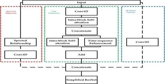
2.3. Model Structure

The structure (Figure 7) of the whole model can be divided into two main parts, namely, the feature extraction of remote sensing time series data and the classification of the ResNet neural network. We had to find the representative features of each category, and then classify the time series data according to these significant features. In our proposed neural network model, we mainly considered four kinds of features of remote sensing time series data, including the local intra-block memory feature, the inter-block correlation feature, the time sequence importance feature, and the spectral sequence correlation feature.

In the structure of our proposed model, the length of the input time series was T, and the characteristic dimension was D. First, the original data are multidimensionalized through a convolution operation, to derive a hidden representation of the input time series. Then, the result of the convolution of the input sequence was sliced up into many subsequences. The subsequence length was BLOCK-NUM, which was set by us. The slicing method started from the first time step of each sample sequence, with 1 as the move step size and BLOCK-NUM as the slice length. Finally, many subsequences with the same shape were obtained. Using the self-attention mechanism in each subsequence, a new sequence that considers the local feature of the element was obtained. Similar to the sequence encoded in the encoder–decoder model to obtain a fixed length semantic vector, our model used a convolution whose kernal size was BLOCK-NUM to obtain the memory feature vector that represents the subsequence. These memory feature vectors of all subsequences were spliced into a new sequence. Lastly, the local intra-block memory feature in the subsequence blocks was extracted.

After that, we passed the sequence that was spliced by all memory feature vectors through a self-attention layer again, and derived a new sequence that introduces the inter-block correlation feature. According to the weight matrix obtained through the process of using the self-attention mechanism among all the memory feature vectors, the importance degree of each block in the time sequence was calculated. By multiplying the sequence spliced by all memory feature vectors by the importance degree vector, we could derive the sequence that introduces the time sequence importance feature. Finally, the sequence that introduces the time sequence importance feature and the sequence that introduces the inter-block correlation feature are added together to combine the two kinds of features. The above operation was carried out on the time dimension. In order to consider the correlation information between various spectral sequences, we used the self-attention mechanism on the spectral dimension of the input sequence. We derived a new sequence that introduces the spectral sequence correlation feature. The input sequence changes dimensions through convolution to splice with the features listed above and derive the final feature sequence. The feature sequence was finally entered into a ResNet network for classification.

2.4. Self-Attention Mechanism

Vaswani, A., et al. [17] proposed the self-attention mechanism for the first time and applied it to machine translation. The model proposed in this paper completely abandons the recurrent neural network and the convolutional neural network, and only uses the self-attention mechanism to deal with the sequence problem, and achieves excellent results.

2.4.1. The Principle of the Self-Attention Mechanism

The difference between the self-attention mechanism and the traditional attention mechanism is that the self-attention mechanism considers the interaction among the various elements within the sequence. The self-attention mechanism mainly includes three parts: A. Calculate the query vector, key vector, and value vector for each time step; B. Calculate the weight matrix; C. Calculate the weight sum [43,44]. Figure 8 shows the structure of the self-attention mechanism.

The expression of the self-attention mechanism is as follows:

Attention(Q,K,V) = softmax(QK^T/√d)V,

(1)

Q, K, and V are the query vector, key vector and value vector, respectively. d is the dimension of the key vector.

The calculation method of these three vectors is as follows:

Q = W_QX

(2)

K = W_KX

(3)

V = W_VX

(4)

X is the data of one time step, and W_Q, W_K and W_V are parametric matrices.

In the process of calculating the weight matrix W, each time step uses its own Q and the transpose of K at other time steps to do a dot product to get a score. After deriving the dot product score for each time step, we input the result into a softmax layer to get the weight of each time step’s influence on the current time step. Finally, each time step was multiplied by the corresponding weight, and then added together to derive a new vector that represents the current time step. As such, each time step receives a new representation.

2.4.2. Intra-Block and Inter-Block Self-Attention

The process of intra-block and inter-block self-attention can be divided into two parts. The first part involves slicing the original sequence and then using the self-attention mechanism in the subsequence. The second part involves using self-attention mechanisms on all the blocks. Figure 9 shows these two parts.

In the processing of subsequence blocks, our method is different from the DP-SARNN proposed by Pandey, A., et al. [24]. Instead of combining RNN and self-attention in SARNN, we used only a self-attention mechanism, abandoning the RNN part of the recurrent neural network, which can greatly reduce the memory occupation and improve the efficiency of the model. In addition, in the self-attention part of the mechanism, the methods of acquiring the Q, K and V vectors are also different from in the DP-SARRN model. In DP-SARNN, layer normalizations are used for obtaining the Q, K and V for each time step, whereas in the model we present, we have used convolution for self-attention [28]. When using this method to obtain Q, K and V, the weight of each time step is shared, which can reduce the training burden of the model compared with the traditional self-attention mechanism.

The model we propose is different from the MCNN proposed in Cui, Z., et al. [8] in terms of the slice method. In MCNN, subsequences of different scales are obtained by the down-sampling of different scales.

In the model proposed by us, the method of acquiring subsequences starts from the first time step of each sample sequence, taking 1 as the move step size and BLOCK-NUM as the slice length.

Each result from the self-attention processing mechanism is added to the original subsequence that is the input of the self-attention mechanism. Then, the result of this addition is convolved into a one-dimensional vector using a convolution layer. This one-dimensional vector takes into account the local features of the subsequence and can be used as the memory feature vector of the subsequence. Finally, all the memory feature vectors are spliced into new sequences. The new sequence passes through the inter-block self-attention mechanism again. This operation allows each subsequence to take into account all other subsequences, thus introducing the characteristics of global information for the entire sequence.

2.5. Time Sequence Enhancement

Time sequence enhancement is inspired by the TCAN model proposed by Hao, H., et al. [25]. The purpose of time sequence enhancement is to find out the important parts of the time dimension, and to enhance this important part and weaken the unimportant part. In the TCAN model, in order to prevent the leakage of future information, the self-attention mechanism does not consider the information of the whole time series, but only considers the sequence information before the current time step. It is reasonable to apply such a self-attention mechanism in the domain of time series prediction. However, it does not apply to time series classification. We suggest considering the data for all the time steps in the time series. As in the classification process, all time steps affect the final classification result.

The time sequence enhancement process uses the weight matrix obtained from the inter-block self-attention process. Figure 10 shows the process.

The input of the inter-block self-attention mechanism is the concatenation, C, of all feature memory vectors. After the inter-block self-attention mechanism, we can derive a new sequence with global correlation characteristics and a weight matrix, W. In this part, we need to use the weight matrix, W. Each of its rows represents the weight of the current block affected by another block. Therefore, W(i,j) represents the influence weight of the j-th block on the i-th block. If we add up all the entries in the j-th column, we can integrate the effect of the j-th block on all the other blocks. Additionally, this gives us a rough idea of the importance of the j-th block in the entire time series. Therefore, we add each row of the weight matrix, W. Then, the result is passed through the softmax layer, and we can derive a one-dimensional vector. Each element in the one-dimensional vector represents the importance of each block.

2.6. Spectral Sequence Relationship Extraction

Wu, Z., et al. [45] introduces the relationship of multi-source data. We know that multispectral remote sensing images contain data for multiple bands. In the multispectral remote sensing time series data, there is a time series in every band of every pixel. Whether or not this means that there is a specific relationship between different spectral time series in a certain land class is debatable. We use the self-attention mechanism in the spectral dimension of the original multispectral remote sensing time series, and make use of the specific correlation among different spectral sequences of each species to classify them.

As every sample is made up of two-dimensional sequence data, the first dimension of the sample is the time dimension, and the second dimension is the spectral dimension. Suppose the data have T time steps and D bands. When the self-attention mechanism is used in the time dimension, the smallest element is a one-dimensional vector composed of D spectral data. The purpose of using the self-attention mechanism in the time dimension is to find the correlation between different time steps. Therefore, in order to find the correlation within the spectral dimension, we need to use the self-attention mechanism on the spectral dimension. When using the self-attention mechanism on the spectral dimension, the smallest element is the T time step data of a spectrum. Accordingly, we can apply the correlation between spectral sequences to the classification of remote sensing time series.

2.7. ResNet

After extracting all the features and fusing them, we input the fused features into a ResNet network. The method of feature fusion involves summing the local features extracted from the self-attention method within every subsequence, the global features extracted from the self-attention mechanism among the subsequences, and the time series enhancement features. Additionally, we then splice the addition results, the spectral sequence relationship features, and the original features to derive the final fusion feature. It should be noted that we only used the idea [46] of residuals, and did not use a very deep network structure. A similar structure is used in our model to the ResNet mentioned in Fawaz, H.I., et al. [6]. Figure 11 shows the structure of the simplified ResNet.

In this structure, we only use three residual blocks to process and classify the fusion features. There are three convolutions in each residual block, and the number of convolution kernels for the three convolutions in the block is the same. The numbers of convolution kernels for each of the three residual blocks are 192, 256 and 256, and each convolution is followed by a batch normalization layer and a ReLu activation layer. Finally, there is a global pooling layer and a softmax layer.

3. Results

In this section, we will introduce the results of experiments conducted on two datasets. Our experimental process includes a comparison among different models and digestion experiments.

3.1. Experimental Setup

We selected some other models for time series classification. These models were long short-term memory (LSTM) and temporal convolutional network (TCN). Figure 12 and Figure 13 respectively show the structure of LSTM and TCN.

The structure of the LSTM was a recurrent neural network LSTM layer. The number of units was 64. After these, there was a batch normalization layer and an activation function layer. The activation function used ReLu. The last was a softmax layer.

For the TCN we used a keras integrated tcn package.

The length of the sub-sequence block in OURS was 6. For the self-attention mechanism, the dimensions of the query vector, key vector and value vector are 64. The numbers of convolution filters in the three residual blocks are 192, 256 and 256, respectively, and the convolution was followed by batch normalization and ReLu activation functions.

Table 4. Hyperparameters.

Methods	Batch	Epoch	Optimizer	Loss	Min-lr
LSTM	64	800	Adam	CE 1	0.0001
TCN	64	800	Adam	CE 1	0.0001
OURS	64	800	Adam	CE 1	0.0001

¹ categorical_crossentropy.

shows the hyperparameters of the models.

In [6], the author used a large number of deep learning network models to classify a large number of time series datasets, and we summarized the hyperparameters of several network models with better classification effects.

3.2. Results on Benchmark Data

We will first introduce the results for the standard dataset.

3.2.1. Result Comparison

We uses the models and parameter settings from Section 2.1 for our experiments. We used the trained model to classify the test set. Finally, we derived the confusion matrix of the classification results of each model.

Table 5. Confusion matrix of LSTM.

Label	One	Two	Three	Four	Five	Six	Seven	Eight	Nine
one	3554	149	87	26	4	110	28	27	15
two	160	342	15	30	5	58	18	2	17
three	84	17	3535	150	16	106	34	34	24
four	17	23	81	3101	128	29	1	0	18
five	11	3	16	144	2398	2	1	0	13
six	42	6	119	35	0	914	12	7	1
seven	23	15	35	3	3	29	1404	15	4
eight	22	7	58	0	0	25	9	31	2
nine	19	22	50	36	10	0	6	3	373

,

Table 6. Confusion matrix of TCN.

Label	One	Two	Three	Four	Five	Six	Seven	Eight	Nine
one	3683	113	68	17	5	44	30	29	11
two	107	503	8	7	1	5	2	6	8
three	63	11	3704	75	23	54	22	26	22
four	9	6	54	3242	72	9	1	0	5
five	4	2	12	51	2514	1	1	0	3
six	18	1	53	10	1	1037	4	12	0
seven	21	6	16	2	1	10	1456	16	3
eight	11	2	17	0	1	6	5	112	0
nine	11	7	20	7	13	2	1	3	455

and

Table 7. Confusion matrix of OURS.

Label	One	Two	Three	Four	Five	Six	Seven	Eight	Nine
one	3797	72	55	4	2	29	25	12	4
two	83	552	2	1	1	1	2	0	5
three	46	11	3790	51	12	42	16	18	14
four	6	4	29	3288	60	3	0	0	8
five	2	0	11	32	2539	0	0	0	4
six	11	0	35	3	1	1076	6	4	0
seven	11	1	14	0	0	5	1494	5	1
eight	6	0	11	0	0	3	1	133	0
nine	9	3	14	3	7	0	0	1	482

show the confusion matrix LSTM, TCN and OURS.

Observing the above confusion matrix table, we can see that no matter the type of land cover, our model gave the most correct divisions.

We used the five evaluation indicators in

Table 8. Evaluation of models on benchmark dataset.

Name	Precision	Accuracy	Recall	F1 Score	Kappa
LSTM	0.7660	0.8709	0.7535	0.8700	0.8445
TCN	0.8716	0.9295	0.8908	0.9299	0.9153
OURS	0.9230	0.9543	0.9349	0.9543	0.9450

to evaluate the above models. Our model performed best on every evaluation indicator.

3.2.2. Digestion Experiment

In this section, we decided to remove some of the branches from our model for comparative experiments. In order to verify them separately, we deleted the self-attention part or the spectral sequence relationship feature part from our model.

For our first model, we removed the self-attention part used in the time dimension, and only retained the relationship characteristics of the spectral sequence. On the contrary, for our second model, we removed the spectral sequence relationship features that operate in the spectral dimension, and retained the self-attention part in the time dimension. In the last model, we removed both these two branches.

Combining Table 8 and

Table 9. Evaluation of models for the benchmark dataset.

Name	Precision	Accuracy	Recall	F1 Score	Kappa
Without attention	0.9142	0.9490	0.9161	0.9489	0.9386
Without spectral relationship	0.9133	0.9516	0.9237	0.9516	0.9418
Without both	0.9058	0.9479	0.9176	0.9479	0.9373
OURS	0.9230	0.9543	0.9349	0.9543	0.9450

, we can see that the single-branch model is better than the LSTM and TCN, but it is not as good as the classification result that combines the features of the two branches. The reason for this may be the feature fusion between different branches, which only compensates for their respective shortcomings and achieves a complementary result.

The model with both branches removed performed better than LSTM and TCN, indicating that the structure of our choice based on ResNet was correct. After introducing our self-attention part and the spectral sequence relationship features, the performance of the model was improved again.

3.3. Result on Self-Selected Dataset

We used trained models to classify the data from the test set. We used the five indicators of “precision”, “accuracy”, “recall”, “f1-score”, and “kappa-score” for evaluation.

From

Table 10. Evaluation of models on self-selected dataset.

Name	Precision	Accuracy	Recall	F1 Score	Kappa
LSTM	0.9135	0.9382	0.9190	0.9386	0.9257
TCN	0.9929	0.9910	0.9870	0.9910	0.9892
OURS	0.9973	0.9984	0.9984	0.9984	0.9981

, we can see that the model we proposed was better than the other models in terms of the classification of the test set. Moreover, we can see that the accuracy of the classification results for the test set is very high. We think that part of the reason is that the remote sensing image range of the dataset we selected was too small. The sample similarity in each category was relatively high, which led to the final classification result being too accurate. However, even so, our model performed better than other models on the same dataset.

We can derive a confusion matrix that uses our model to classify the test set.

Table 11. Confusion matrix of OURS for the self-selected test set.

Label	Bare Land	Woodland	Water	Arable	Building	Rock	Road	Grass
Bare land	299	0	0	0	0	0	1	0
Woodland	0	599	0	0	0	0	0	0
Water	0	0	522	0	0	0	0	0
Arable	0	0	0	107	0	0	0	0
Building	0	0	0	1	538	0	0	1
Rock	0	0	0	0	0	121	0	0
Road	0	0	0	0	1	0	177	0
Grass	0	0	0	0	0	0	0	190

shows the confusion matrix of our model’s classification results on the test set.

We used the trained model to forecast and classify the original 900 × 750 pixel points, and used the predicted results to derive a distribution map for the whole remote sensing image.

Figure 14 shows the prediction classification results of the original 900 × 750 pixel points.

The above classification results show that the LSTM model is very suitable for the classification of roads.

The LSTM module in Figure 15 shows the roads in more detail. On the other hand, our model blurs some dense road areas.

However, there are deficiencies in the distinction between bare land and cultivated land. For example, in Figure 16, we can see that the LSTM model incorrectly classified some types of bare land as cultivated land.

The accuracy of the TCN model on the test set was similar to that of our model, but still lacked quality in some places. For example, in Figure 17, we can see that the TCN did not divide the entire road, but divided the back part of the road into buildings.

4. Discussion

Whether it is on a standard dataset or a dataset of our choice, we can come to the conclusion that the combination of the self-attention mechanism and the correlation among multiple bands is beneficial to the time series classification of remote sensing data.

In this section, we will use the results obtained on the standard dataset to further explain the features of each part of the branch we proposed. We will first introduce the correlation features of the spectral sequence, and then the inter-block feature matrices and time sequence enhancement features of the self-attention part.

4.1. Spectral Sequence Relationship Feature Visualized Analysis

For multi-band remote sensing time series, the self-attention mechanism is used in the band dimension to obtain the relationship among each band sequence, and we have visualized this relationship. Figure 18 shows the visualization of spectral sequence relationship feature.

Overall, we see that the eighth band (NDVI) has the lowest impact on the other bands. In the four types of samples, forests, grassland, other crops and sugarcane crops, there are similarities in the distribution maps of the impact levels between the bands. The reason for this may be that all four types of land cover have green plants. This leads to similar distribution diagrams amongst the various bands.

The band relationship distribution maps of urban areas, other built-up surfaces, rocks, and bare land are also similar. The reason for this may be that the other built-up surfaces category includes some surface coverage similar to urban areas, such as some similar buildings. Moreover, there are some impervious objects in these three categories. Finally, water and sparse vegetation behave very differently from other surface coverage categories.

4.2. Inter-Block Self-Attention Matrix Visualized Analysis

In the process of global feature extraction, we use the degree of influence among the different subsequence blocks of each sample. In the model training process, this feature can be expressed as a weight matrix. For different types, their respective weight matrices should be different. Therefore, through the output and visualization of the intermediate results of the model, we have obtained visualizations of the weight matrices of different types of features. In the distribution diagram, the darker the color, the smaller the degree of influence. Figure 19 shows the visualization of the Inter-block self-attention matrix.

For each type of land cover, we selected the inter-block influence matrix of two samples for visualization. Although the distribution diagrams of different samples in the same category are not the same, we found two similar distribution diagrams for each category through selection.

Although there are similarities in the spectral relationship distribution diagrams, we can see some differences in their inter-block influence matrix distribution diagrams. For example, there are differences in the distribution maps of urban areas and other built-up surfaces. In the distribution map of urban areas, the area (13–18, 13–18) is brightly colored, which means that the mutual influence is greater; in the distribution map of other built-up surfaces, in (6–7, 0–18) and (12–13, 0–18), two areas show two obvious dark bands. Although there are dark bands in the distribution maps of forests and grassland at (7, 0–18), there are obvious dark areas in the distribution maps of forests at (12–15, 0–11). However, this dark area does not exist in the distribution map of grassland.

In addition, sparse vegetation and water are still the easiest to distinguish from other types of land cover. In the distribution graph of sparse vegetation, there is a dark band at (0, 0–18). The overall distribution of water is brighter.

4.3. Time Sequence Enhancement Feature Visualized Analysis

In the process of time sequence enhancement feature extraction, we can find the importance of each subsequence block in terms of timing. In the same way, we can output the intermediate results of the model and derive the timing importance curves of different types. Figure 20 shows the visualization of the time sequence enhancement feature.

In a sense, the timing importance curve exhibits a strong relationship with the inter-block influence matrix between the blocks. If a certain column in the inter-block influence matrix is a dark band, then the corresponding position on the timing importance curve will have a relatively low value.

In the timing importance curve, we can also see some differences between different samples. For example, where the horizontal axis of the timing importance curve of the forests sample is equal to 7, or is within the range of 12.5–15, the curve is at a low peak. However, there is a peak in the range of 3–5 or the range of 8–12. In the range of 5–7 or 10–12 on the timing importance curve of rocks and bare soil, the value is significantly low. The sample timing importance curve of sparse vegetation maintains a relatively high value above 9.

5. Conclusions

In our proposed model, we need to extract sample features from each time series sample. The method of extraction is to obtain the memory feature vectors of the subsequence first, and then to use the self-attention mechanism among the feature vectors of the subsequence. Therefore, the processing of a subsequence takes into account the local and global features of the time series. Then, we use the self-attention mechanism on the spectral dimension of remote sensing data to determine the relationship among each band of the time series. The fusion of these features imbues our final sequence with more comprehensive information. However, when our model is used to extract the relational features of spectral sequences, we just use a simple self-attention mechanism. This method does not obtain the characteristics of spectral sequence relations perfectly.

Considering the current rapid development of graph convolution, we will consider applying graph convolution in the extraction of the relationship between various spectra in the next work. Different bands can be considered as different nodes, and thus graph convolution can be used to utilize the characteristics of the relationship between the various bands.