Eddies in the Marginal Ice Zone of Fram Strait and Svalbard from Spaceborne SAR Observations in Winter

Abstract

Here we investigate the intensity of eddy generation and their properties in the marginal ice zone (MIZ) regions of Fram Strait and around Svalbard using spaceborne synthetic aperture radar (SAR) data from Envisat ASAR and Sentinel-1 in winter 2007 and 2018. Analysis of 2039 SAR images allowed identifying 4619 eddy signatures. The number of eddies detected per image per kilometer of MIZ length is similar for both years. Submesoscale and small mesoscale eddies dominate with cyclones detected twice more frequently than anticyclones. Eddy diameters range from 1 to 68 km with mean values of 6 km and 12 km over shallow and deep water, respectively. Mean eddy size grows with increasing ice concentration in the MIZ, yet most eddies are detected at the ice edge and where the ice concentration is below 20%. The fraction of sea ice trapped in cyclones (53%) is slightly higher than that in anticyclones (48%). The amount of sea ice trapped by a single ‘mean’ eddy is about 40 km², while the average horizontal retreat of the ice edge due to eddy-induced ice melt is about 0.2–0.5 km·d^–1 ± 0.02 km·d^–1. Relation of eddy occurrence to background currents and winds is also discussed.

1. Introduction

Eddies forming at the ice edge and within marginal ice zones (MIZ) are a common dynamic feature of the ice edge evolution under varying winds and ocean currents in polar oceans. They are known to be important for sea ice deformation, horizontal transport and melting. Previous studies show that MIZ eddies are common in polar ocean regions, such as Fram Strait, and discuss the broad variety of their generation mechanisms from available in situ, aircraft and satellite observations [1,2,3,4].

Recent studies also show that polar MIZs are rich in submesoscale flows with high Rossby numbers and strong ageostrophic effects [5,6,7,8,9,10]. Submesoscale ocean variability induces large vertical velocities bringing warm subsurface waters into the mixed layer and results in pronounced ocean-sea ice heat fluxes localized over cyclonic eddies and filaments reaching about 100 W m⁻² [8]. It also leads to enhanced mixing of water masses over short horizontal scales, so impacting the sea ice and biological structures within the MIZ [10].

Available eddy observations in the Arctic Ocean are still very sparse, and hence high-resolution hydrodynamic models are used to fill these gaps [11,12,13,14,15]. Though current state-of-the-art 1 km and finer resolution models potentially resolve small eddies in the MIZ and around sea ice leads [13], a realistic forecasting of meso- and submeso-scale MIZ dynamics is still challenging and needs a good observational basis for model improvement and validation. In this sense, satellite remote sensing using spaceborne synthetic aperture radar (SAR) is a good and effective source of information to explore and better understand the eddy field in the Arctic Ocean, including the ice-covered regions [1,3,7,10,16,17,18,19]. What is especially good about SAR is that it can map MIZ dynamics, including eddy motions, under broad variety of wind speeds including high wind conditions [1,10].

Historically, the eddies forming in the Fram Strait (FS) MIZ obtained a lot of attention during a set of specialized experimental programs such as MIZEX’83, ’84 that used a variety of observational techniques including in situ, satellite and aerial remote sensing (e.g., [1,2,3]). Here MIZ eddies occur in the region where two very different water masses co-exist, namely the cold Polar Water (PW) going with the East Greenland Current (EGC) southward and the warm Atlantic Water (AW) carried by the West Spitsbergen Current (WSC) northward. The latter splits into two recirculation branches interacting with the cold EGC, and Svalbard and Yermak branches entering the Arctic Ocean (Figure 1). Such a close occurrence of the cold PW, the warm AW with very high levels of eddy kinetic energy [13,14,19], and the year-round MIZ creates very favorable conditions for intensive eddy generation [1,7].

Though previous studies in FS gained much information about eddy generation mechanisms, their spatial and kinematic properties and influence on sea ice, the obtained results were still episodic and resolving only a limited number of eddies. The only work reporting a detailed statistics of MIZ eddies in FS and the Greenland Sea using Envisat ASAR data of 2008 and 2009 is that of Bondevik [18]. According to [18], the maximum occurrence of MIZ eddies takes place in summer when the ice extent is near its minimum, while generation and surface manifestation of eddies is favored at relatively low winds of predominant northern direction. In that work, the regions north and northeast of Svalbard, as well as coastal regions around it were not considered.

The aim of this study is to analyze the intensity of eddy generation and document their properties over the region of 74°–83° N and 20° W–40° E (Figure 1), while also assessing their influence on ice trapping and ice edge retreat, and discussing relation to background currents and winds using historical Envisat ASAR and contemporary Sentinel-1 SAR observations in winter season.

2. Materials and Methods

To investigate eddy signatures in FS and around Svalbard we analyze SAR C-band images acquired by ENVISAT Advanced SAR (ASAR) in winter 2007 (December 2006–March 2007) and Sentinel-1 A/B in winter 2018 (January–April 2018). These two winter seasons were selected primarily due to better data availability without much consideration about the sea ice and hydrographic conditions that were somewhat unusual in the study region, as discussed below.

For the analysis we use 212 ASAR images acquired in wide swath mode and image mode with spatial resolution of 150 m and 30 m, respectively. For Sentinel-1 A/B, we use 1827 images taken in interferometric wide swath and extra-wide swath modes with spatial resolution of 20 m and 90 m, respectively. For both data sets we use all publicly available data for the considered time periods. Envisat ASAR data were obtained from the European Space Agency rolling archive, while Sentinel-1 A/B data were obtained from Copernicus Open Access Hub (https://scihub.copernicus.eu (accessed on 1 July 2021). A summary of the data used, their quantity and time periods are given in

Table 1. Number of spaceborne SAR images used in the analysis during winter 2007 and 2018.

Year	Sensor	December	January	February	March	April	Total
2007	ASAR	13	69	52	78	-	212
2018	S-1 A/B	-	500	418	383	526	1827

.

As seen from Table 1, the total number of SAR images analyzed in winter 2018 is nearly 9 times larger than that in 2007. The number of images also varies from month to month in both years, but not significantly. Figure 2 shows the spatial coverage of the study site by SAR data in 2007 and 2018. The maximal density of SAR observations in 2007 is about 70–90 scenes per unit area over the northern Greenland Sea, while for the rest of the region the mean value is about 40 images per unit area. In 2018, the overall density of SAR observations is much higher than in 2007, yet somewhat less homogeneous. The highest image density is found over the northern FS and north of Svalbard where it exceeds 200 images per unit area, in other regions it varies from 30 to 150 images per unit area. Such a big difference in spatial SAR data coverage between 2007 and 2018 is primarily linked to availability of two Sentinel-1 sensors and their more frequent sampling compared to Envisat ASAR. In addition, also note that ASAR has a very poor coverage north of 80° N and east of 10° E which is critical for eddy observations in this important region.

It is also important to note that the season-mean ice margin length and position are different between 2007 and 2018 (Figure 2). In particular, the ice margin is found much further north of Svalbard and there is a much larger ice field southeast of archipelago in winter 2018. As a result, the mean MIZ length is ~3430 km in winter 2007 and ~4160 km in winter 2018, i.e., 1.2 times longer in 2018 than in 2007.

Under light to moderate winds the morphology of the marginal ice zone reflects the underlying ocean circulation, including eddy features [3]. Eddies in the MIZ and at the ice edge are visible in spaceborne SAR images owing to spatial redistribution of drifting ice fields tending to accumulate in the surface current convergence zones associated with spiraling motion of eddy-induced currents [1].

SAR manifestations of MIZ eddies depend on background wind and thickness of drifting ice. In this case thinner ice (e.g., newly forming or melting ice) would be seen in SAR image as dark patterns (low backscatter), while thicker ice fields—as bright patterns (high backscatter). This is well illustrated in Envisat ASAR image acquired on 23 February 2007 over the 50–60 km wide MIZ in Fram Strait (Figure 3). As seen, very dark eddying patterns are seen further off the pack ice that has nearly uniform gray background in the upper left part of the image. Closer to the pack ice, eddy signatures have higher backscatter due to entrainment of more and thicker ice floes in their centers. The distance between the centers of adjacent eddies range from 10 km to 50 km, 30 km on average. Note also numerous bright elongated filaments that are formed due to enhanced ice accumulation in the surface current convergence zones and outline eddy boundaries. The visual inspection of such eddy-induced regions of enhanced/decreased radar backscatter shows the limits of the areas with positive or negative vorticity linked to eddy structures [7].

Our method for eddy detection in SAR data is based on visual identification of their surface signatures frequently used in similar studies [18,20,21,22]. Earlier, it was successfully applied to quantify eddy properties during summer periods in the Western Arctic [23], northern Greenland Sea and Fram Strait [24,25], Barents, Kara and White seas [16]. In order to obtain a coherent pan-Arctic climatology of eddy properties, here we use the same visual detection of eddies in SAR data.

Following the methodology described in [23], every SAR image was visually inspected at full resolution in search for distinct eddy signatures and identification of their boundaries. Then by looking at eddy boundaries outlined due to accumulation of floating ice, their location and vorticity sign (cyclone/anticyclone) were defined manually. The mean of the two quasi-perpendicular sections across the eddy center was taken as a mean eddy diameter.

Analysis of ASAR data was performed using Matlab-based software suggested in [26], while the analysis of Sentinel-1 data was performed using the open-source ESA SNAP software (http://step.esa.int/main/toolboxes/snap (accessed on 14 February 2021). The entire procedure of data pre-processing and eddy detection was similar for all the data. The original SAR data were calibrated to normalized radar cross-section units and smoothed to reduce the speckle noise using Lee filter [27].

The background sea ice concentration corresponding to each eddy center was obtained from daily AMSR-E and its successor AMSR-2 sea ice concentration maps produced by the University of Bremen [28], while a detailed estimate of the amount of sea ice entrained into the eddies was derived directly from SAR images. Depth values corresponding to eddy center coordinates were retrieved from IBCAO Version 3.0 [29]. To analyze the relation of eddy generation intensity to background winds and ocean currents we used ERA Interim Reanalysis 10 m winds and CMEMS GLORYS12V1 reanalysis data for January–April 2018, respectively. For ocean currents’ data we used the surface layer at 0.5 m depth.

3. Results

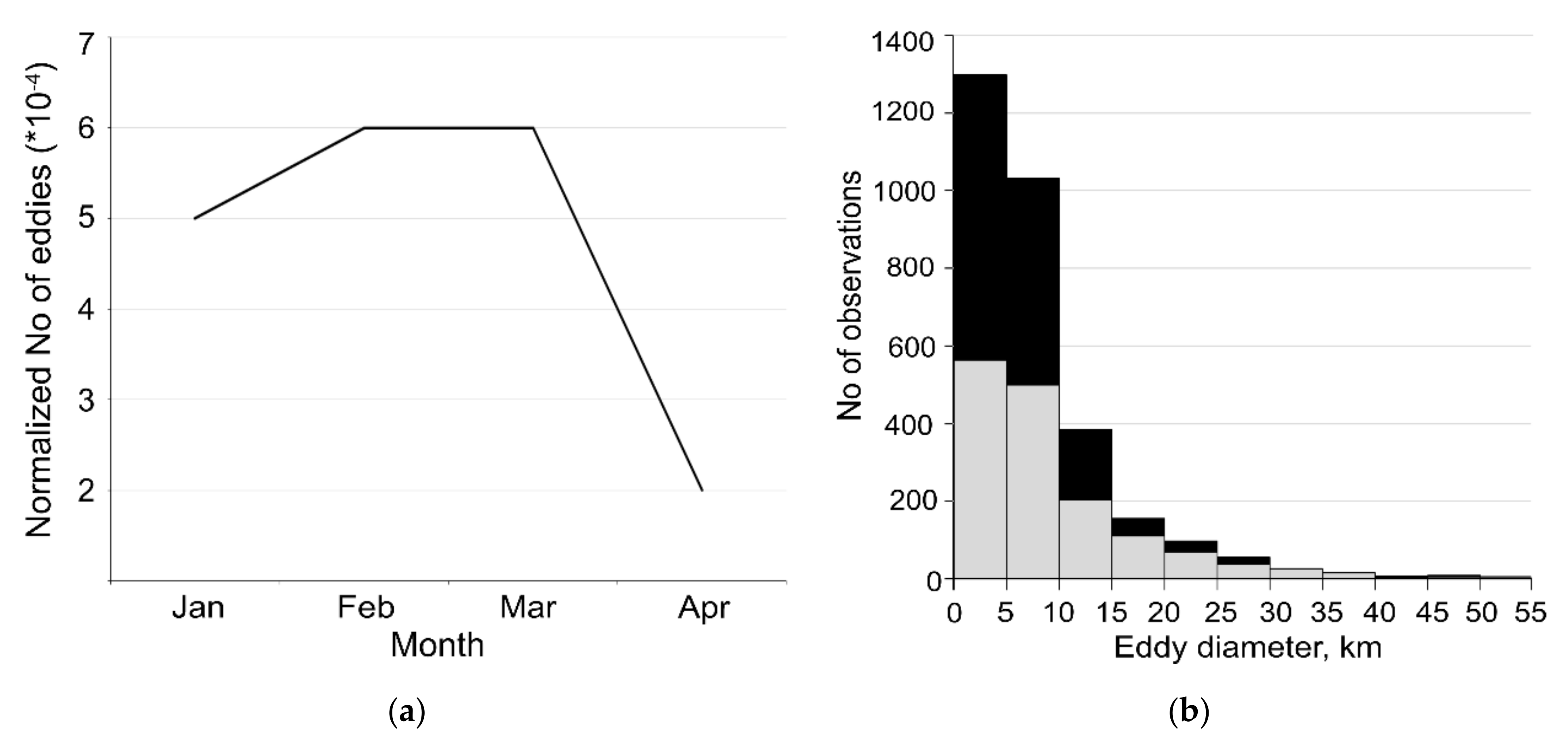
3.1. Spatio-Temporal Statistics of MIZ Eddies

Analysis of spaceborne SAR data for two winter periods of 2007 and 2018 allowed identifying 4619 eddy signatures in the MIZ and at the ice edge with 399 eddy signatures detected in December 2006–March 2007, and 4220—in January–April 2018. Quantitatively, two Sentinel-1 sensors captured 10.5 times more eddies compared to Envisat ASAR, or 1.2 times more eddies when normalized on the number of available SAR images. However, when accounting for the 1.2 times difference in total MIZ length between 2007 and 2018, the average number of eddies detected per one image per kilometer of MIZ length is similar in 2007 and 2018 and does not depend much on the sensor used.

Apart of MIZ eddies, open-ocean eddies were also detected in the data, however, their number was surprisingly small, only 323 eddy signatures. In contrast, much more open-ocean eddies (1609 eddies) were detected in July–September 2007 [24,25]. Such a pronounced difference in open-ocean eddy detections between winter and summer seasons could be related to the less pronounced vertical stratification and the higher near-surface winds during winter months that limits eddy identification in SAR images [18]. Hence, we did not consider open-ocean eddies in the analysis.

Table 2. Summary of the MIZ eddy detection in spaceborne SAR data in winter seasons of 2006/2007 and 2018.

Month	Number of Eddies						Mean Diameter (STD), km
	C		AC		SUM		C		AC		SUM
	2007	2018	2007	2018	2007	2018	2007	2018	2007	2018	2007	2018
December	31	-	7	-	38	-	11.2	-	12.3	-	11.4	-
January	56	752	13	410	69	1162	8	7.5	9.4	9.3	8.3	8.1
February	83	848	40	432	123	1280	11.4	7.1	14	9.5	12.2	7.9
March	109	767	60	424	169	1191	9.7	8.1	12.8	8.2	10.8	8.1
April	-	430	-	157	-	587	-	9.3	-	11.3	-	9.9
Total	279	2797	120	1423	399	4220	10 (8.1)	7.8 (7.2)	12.8 (10.8)	9.2 (8.5)	10.9 (9.1)	8.3 (7.7)

provides a summary of eddy detection results in MIZ obtained upon the processing of all SAR data.

What is immediately apparent, the number of cyclones is twice larger than that of anticyclones (AC), i.e., 67% of C versus 33% of AC, similar for 2007 and 2018. This exactly matches the results of the summer-time observations of MIZ eddies in the Western Arctic [24], and is slightly less than was obtained in the Greenland Sea [18].

In terms of monthly variability, both records show the highest number of eddies in February and March (Table 2). This is also confirmed by the number of eddies detected per given month normalized by the SAR coverage during that month (Figure 4a) and shows similar high values in February and March, a bit lower value for January and a minimum in April.

Table 2 also shows mean values of eddy diameters in 2007 and 2018 and their standard deviations (STDs). The minimum (maximum) value of eddy diameters registered in 2007 is about 1.3 km (66.8 km). In 2018, the minimum diameter value, ~0.6 km, is lower than in 2007 due to higher spatial resolution of Sentinel-1 data, while the maximum is nearly the same, 67.6 km. Large intervals between minimum and maximum values of eddy diameters in 2007 and 2018 explain high STDs in the record.

Figure 4b shows a histogram distribution of eddy diameters for eddies registered in winter 2018. Both cyclones and anticyclones have a peak in the range of diameters of 1–10 km. It is also apparent that at scales of 1–15 km cyclones strongly dominate over anticyclones. However, in the range of 15–30 km this difference is gradually vanishing, and for diameter values above 30 km anticyclones start to dominate slightly. This appears to be a characteristic feature previously documented for open-ocean eddies detected in SAR images elsewhere [22,30].

Figure 5 shows a spatial distribution of MIZ eddies detected in 2007 and 2018, and their probability calculated on a 35 km × 35 km grid as the ratio between the total number of eddies encountered within a given grid cell and the number of SAR looks of that cell. The probability color bars in Figure 5c,d have a maximum at 0.2 which means that at the particular grid cell at least one eddy is registered in every fifth SAR image. Note that at some locations the maximal probability values exceed this upper limit.

In 2007, the eddies were identified across the narrow band (hereinafter, Fram band) extending over 75°–80° N and 10° W–4° E (i.e., the region of maximum SAR coverage in 2007), in Great Fjord Strait and over the Spitsbergen Bank (Figure 5a).

The results for winter 2018 confirm and expand the above results for 2007. A very dense and 200–250 km wide band of eddy detections, resulting from the gradual week-to-week variability of the ice edge location, now expands all along the Greenland Sea shelf break and slope, Fram Strait, southern Yermak Plateau (YP) and further east up to 40° E over the deep water north of Svalbard (Figure 5b). These regions are also characterized by the highest probability of eddies of 0.2 and higher (Figure 5c,d).

Many eddies are also registered over the Spitsbergen Bank and in the coastal regions around Svalbard, in many fjords and straits, especially in the southern part. The highest probability of eddies is found east of Edge Island, around Hopen, Prince Karl Land and Bear Islands, and near the southern tip of Spitsbergen. The most pronounced hot spot of MIZ eddy generation is the region over the Spitsbergen Bank and near Hopen Island. The barotropic tidal currents are strong here [31,32], reaching 20 cm/s, and the eddies are generated due to instability of sheared current when the flow passes the orographic obstacle [33]. High eddy probability is also found in Great Fjord Strait, where frequent eddy generation was also reported in summer [25], and could be related to interaction of cold PW entering through Heleisund and Freeman straits and warm AW coming with the WSC.

From the comparison of two data sources one can clearly see that the ASAR-based eddy observations in winter 2007 partly lack some important regions of frequent eddy generation observed by Sentinel-1 in winter 2018, e.g., north of Svalbard and in many coastal areas around it. Of course, the observed difference results not only from a much wider coverage of the study site by Sentinel-1 data, but is also related to rather different sea ice extent and ice margin location in 2007 and 2018 (see Figure 2).

Figure 6 shows a spatial distribution of mean and maximum values of eddy diameters on the 35 × 35 grid for 2007 and 2018. Comparison of mean values for 2007 and 2018 (also shown in Table 2), where they overlap, suggests that higher mean values were observed in 2007. This is particularly pronounced at 76–79° N where mean eddy diameters of ~20–25 km are observed in 2007 versus ~12–20 km in 2018.

However, it is not the case for the maximum eddy diameter values (Figure 6c,d). Where observational data of 2007 and 2018 overlap, the data of 2018 have, in general, higher values. Moreover, there are at least three hot spots in Fram eddy band (75°–80° N) where eddy diameters are of 40–60 km, while only one is seen in 2007 (marked by red boxes in Figure 6c,d). There are also other hot spots of high eddy diameters—over the southeastern YP and further eastward.

Figure 6 also clearly shows the overall difference in eddy diameters between the deep and the shallow regions with larger eddies usually found over the deep water. This is detailed in Figure 7a showing a distinct increase in eddy diameters from about 6–7 km over <500 m depths to maximum values of 11–15 km over 2000–3000 m depths, and another pronounced decrease for deeper regions.

According to [34], the first mode Rossby radius is about 5–8 km over the deep-water regions of the Greenland Sea, Fram Strait and north of Svalbard in winter, and about 0.5–3 km in the shallow coastal regions around Svalbard. In our case, the observed mean eddy radii are about 3 km in shallow water and 5–7.5 km in deep water, suggesting that submesoscale and small mesoscale eddies dominate in the record. Indeed, the portion of submesoscale eddies for shallow water (i.e., eddies with radii <3 km) is 69% out of 2121 eddies, and 57% out of 2168 eddies found over deep water (i.e., eddies with radii <5 km).

Note also that anticyclones (gray curve in Figure 7a) are always 15–30% larger in diameter than cyclones (black curve in Figure 7a), which is also well seen from Table 2 for all months and years. This, again, appears to be a common feature in the Arctic Ocean [16,23] and elsewhere [22,33,35].

Figure 7b provides a general information about the background ice concentration at the locations of MIZ eddy encounters in 2007 and 2018. Clearly, most eddies were detected at the ice edge and in the regions with the low ice concentration (<20%). Once the ice concentration rises above 10%, the number of detected eddies rapidly drops down with the minimum found around 60–90% of the ice concentration. Interestingly, a small rise of eddy detections is also seen over the pack ice with the ice concentrations of 90–100% which makes it different from the results obtained in the Western Arctic in summer [23]. Another remarkable feature is that the size of detected eddies apparently rises with increasing ice concentration, especially prominent for cyclonic eddies (Figure 7b). Plausibly, the increase of mean floe size with increasing ice concentration in the MIZ limits the detection of small eddies under pack ice compared to low ice concentrations.

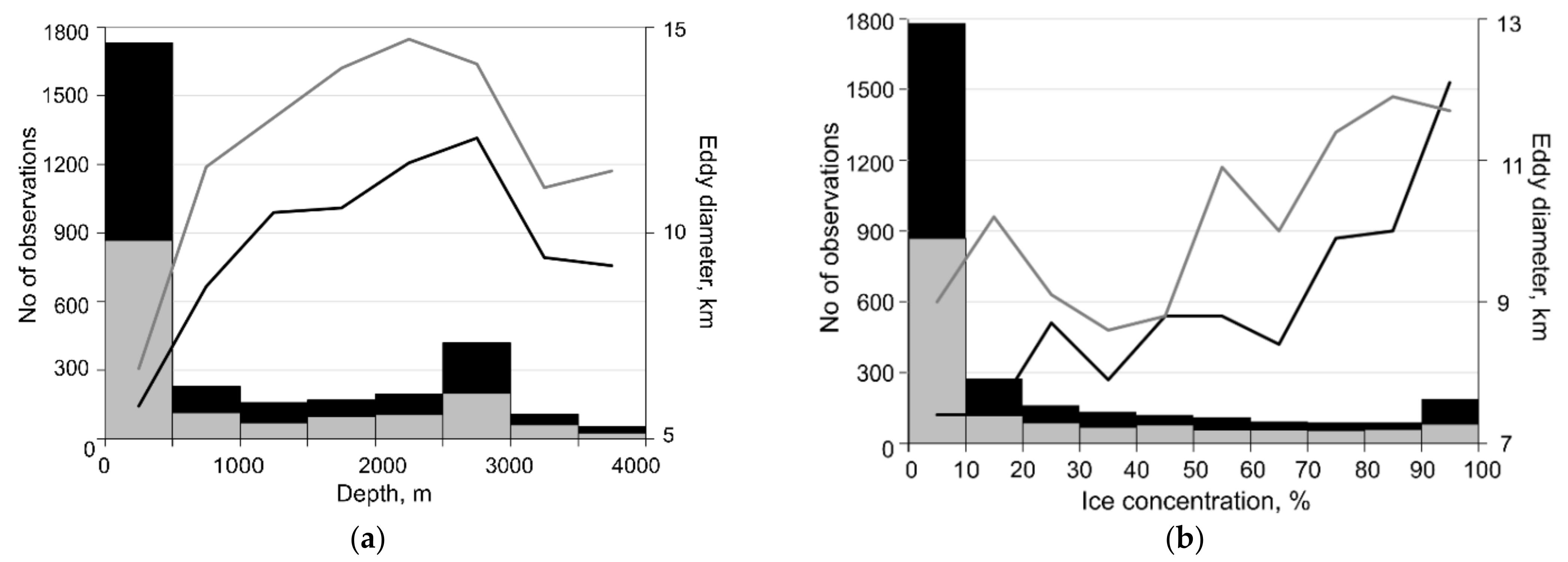
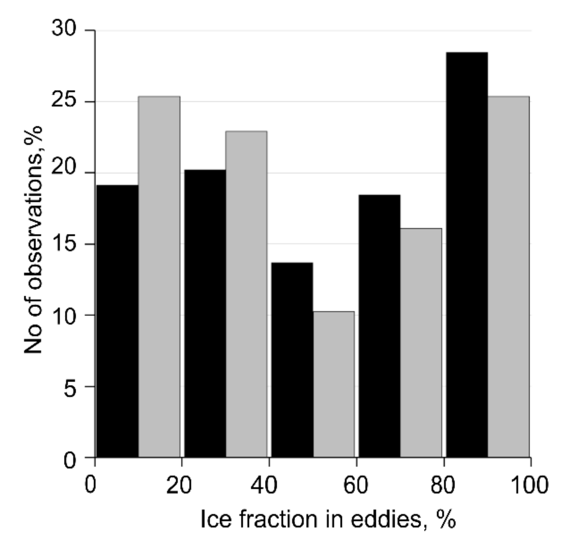
3.2. Ice Trapping and Melting by Eddies

Figure 8 further shows a histogram distribution of sea ice fraction inside detected eddies derived from SAR images. This property was counted only for eddies detected in January 2018 (1162 eddies), presuming that it should be relevant for the entire record. It describes the amount of sea ice trapped inside every single eddy. The ice fraction in eddies was visually estimated using five classes from 0% to 100% with a 20% step in sea ice concentration. For this, every eddy was zoomed at full resolution, and then a curve following the eddy boundaries and two perpendicular lines denoting the eddy diameter were put on. A relative amount of ice within the eddy was then evaluated visually and assigned to one of five classes with mean ice concentration values of 10%, 30%, 50%, 70% and 90%.

Bearing in mind that cyclones were twice more frequent than anticyclones, the number of observations for cyclones (anticyclones) in Figure 8 is given relative to the total number of cyclones (anticyclones), not the total number of all eddies, so that their histogram distributions would be easily comparable. As seen from Figure 8, the distribution for cyclones (black bars) has peaks in two classes of 20–40% and 80–100% with higher number of observations in the latter. For anticyclones (gray bars), two equal peaks are in 0–20% and 80–100% classes with an overall higher portion of observations for ice fraction values below 50%. Indeed, the mean value of ice fraction for anticyclones is slightly lower (48%) than that for cyclones (53%). Hence, below we take the mean ice fraction in eddies equal to 50%.

Bondevik [18] used the same value of mean ice fraction of 50% and mean eddy radius of 30 km to quantify the area of sea ice trapped by a single eddy and associated integral eddy-induced retreat of the ice edge. Our results suggest a much smaller range of mean eddy radii, 3–7 km. Following [1,18] and taking the mean eddy radius $r=$ 5 km, and the mean ice fraction $f=$ 0.5 (i.e., 50%) results in trapping of $S_{ice}=\pi r^{2}f=3.14\times 5^2\times 0.5~$40 km² of sea ice by a single ‘mean’ eddy, i.e., about 40 times less than estimated in [18].

In general, MIZ eddies can persist from couple of days till several weeks [1,7]. Assuming that each eddy was detected in SAR data at least twice (but could be more frequent), the average number of eddies per winter month equals to ~500 eddies. As a result, a total area of sea ice trapped by all eddies per month equals to ~2 × 10⁴ km².

Using the obtained information one can estimate an average horizontal retreat of the ice edge due to MIZ eddies following a simple formula suggested in [1] and applied in [18] in the form:

$$A=\left(\omega f\pi r^2\right)/\left(lh\right)$$

(1)

where $\omega =$ 0.38 m·d^–1 is the mean bottom ablation [36], $f=$ 0.5, $r$ has range of 3–6 km for shallow and deep water; $l$ is the mean distance between the centers of adjacent eddies taken as 15 km for shallow water and 30 km for deep water, respectively; and $h=$ 1.5 m is the mean ice thickness [1,18]. When using Equation (1), we assume that all parameters are constant apart of $r$ that has error ${\sigma }_r\approx$ 0.1 km (i.e., equal to the spatial resolution of the data that is 2 × pixel size $\approx$90 m). To calculate the error propagation, Equation (1) can be presented in the form $A=b{r}^2$, where $b=\left(\omega f\pi \right)/\left(lh\right)$ is a constant value. The relative error is then ${\sigma }_A/A=2{\sigma }_r/r$, and the error of $A\approx$ 0.02 km·d^–1. In this case, the average horizontal retreat perpendicular to the ice band equals to 0.2–0.5 km·d^–1 ± 0.02 km·d^–1.

Having spatial fields of some parameters (i.e., $f$ and $r$) used in Equation (1) on the 35 × 35 grid, it is a natural step to obtain a spatial distribution of $A$ first for January 2018 and then for the entire winter 2018. To calculate $A$ for January 2018 we use ice fraction in eddies, $f$ (Figure 9a), and eddy radii, $r$ (Figure 9b), on the 35 × 35 grid derived from SAR observations, the mean distance between the centers of adjacent eddies equal to 15 km (depth < 300 m) and 30 km (depth > 300 m), and other parameters as constants described above.

Note that ice fraction in eddies (Figure 9a), in general, has higher values over the Fram eddy band, 0.5–0.8 (or 50–80%), and a similar range of values over the northern band and the Spitsbergen Bank near Hopen, 0.2–0.6 (20–60%). For the entire winter of 2018 (Figure 9d), only $r$ is taken on the 35 × 35 grid ($r=d/2$ with the spatial distribution of $d$ shown on Figure 6b), and the distance between adjacent eddies varies depending on depth, while other parameters are constant (including $f=$ 0.5).

According to calculations, in January 2018, high values of horizontal ice retreat, up to 1.5–2 km·d^–1, are seen over the southern part of the Fram eddy band, between 74–79° N, and over the slope regions northeast of Svalbard and YP (Figure 9c). These regions are characterized by relatively high values of eddy radii and ice fraction inside eddies as compared to adjacent regions (Figure 9a,b). Minimal $A$ values about 0.1–0.2 km·d^–1 are seen in the coastal regions of Svalbard and over the central and eastern YP, while moderate values (0.3–1 km·d⁻¹) are found over the northern eddy band (southern flanks of YP) and northeast of Hopen Island.

The color lines in Figure 9c show the ice edge location taken from AMSR-2 data in the beginning (5th), middle (15th) and end (25th) of January 2018. As seen, during the month the ice edge boundary has moved either westward (for the Fram eddy band) or northward (for the northern band and over the Spitsbergen Bank), meaning a decrease in the actual MIZ area that could be at least partially attributed to the eddy-induced ice melt. The strongest decrease of MIZ area and shift of the ice edge location are seen during the first part of January (compare the location of red and pink lines), confirming that MIZ possess a strong week-by-week spatial variability. While the ice edge has partially restored back in some locations during the second half of January 2018 (compare red and green lines), the resulting area of MIZ has obviously decreased during the month. However, the amplitude of the ice edge movement does not entirely correlate with the plotted $A$ values, though in some locations the correspondence is still observed.

The distribution of the horizontal ice edge retreat for the entire winter 2018 (Figure 9d) has many similar patterns to its distribution in January 2018 with higher $A$ values observed over the southern part of the Fram eddy band and at some certain locations north, east and south of Svalbard. The spatial distribution of $A$ values in Figure 9d is proportional to eddy size distribution shown in Figure 6b and basically suggests that larger eddies would have a stronger impact on the ice edge retreat in the MIZ. Due to longer time period and rather complex MIZ variability, here we do not attempt to make a direct comparison of $A$ values plotted in Figure 9d with the ice edge locations throughout the 4-month period. Obviously, such a comparison is a very challenging task and would need a lot of additional information about the coupled ocean–ice–atmosphere state in the study region. Nevertheless, the presented methodology allows one to make a kind of sensitivity tests and a bulk estimate of eddy influence on the ice edge retreat in the MIZ.

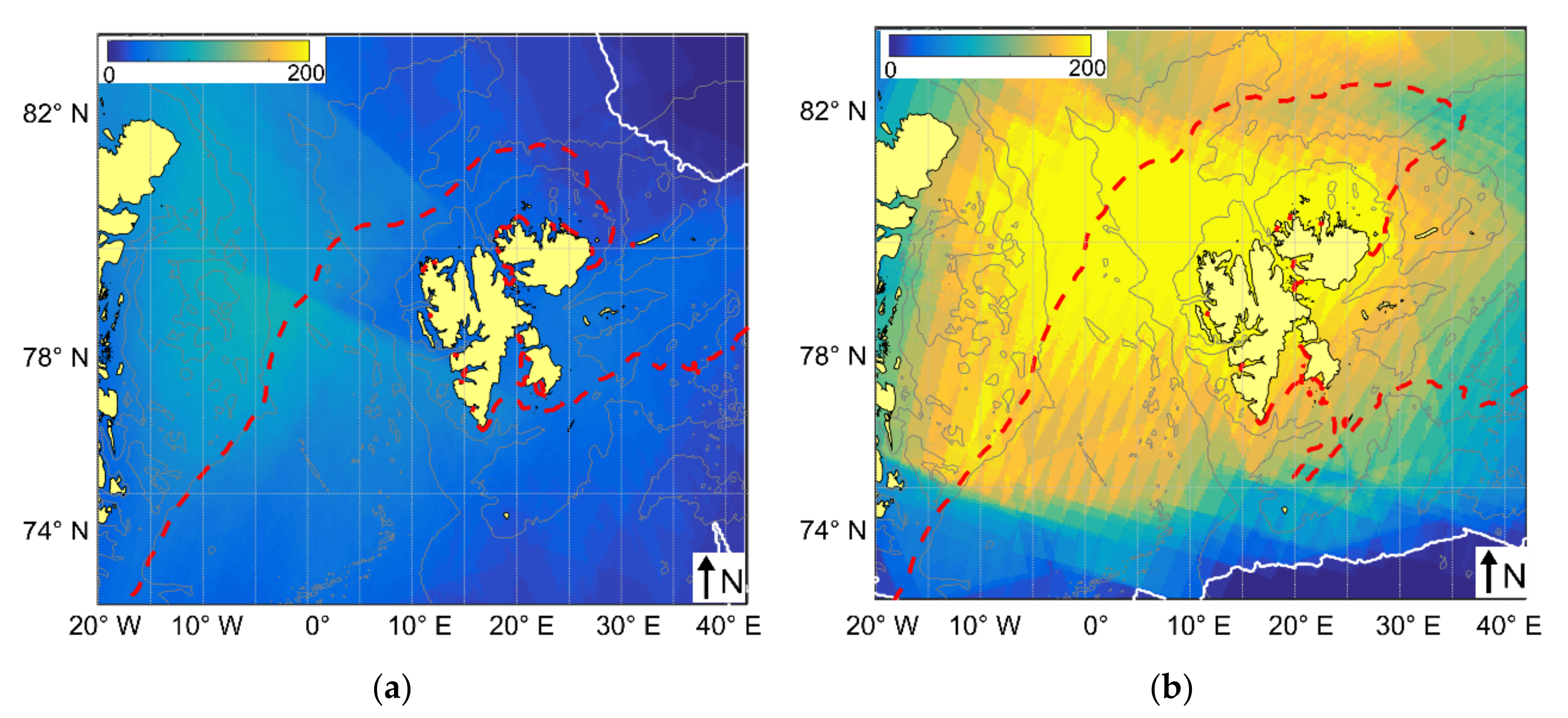
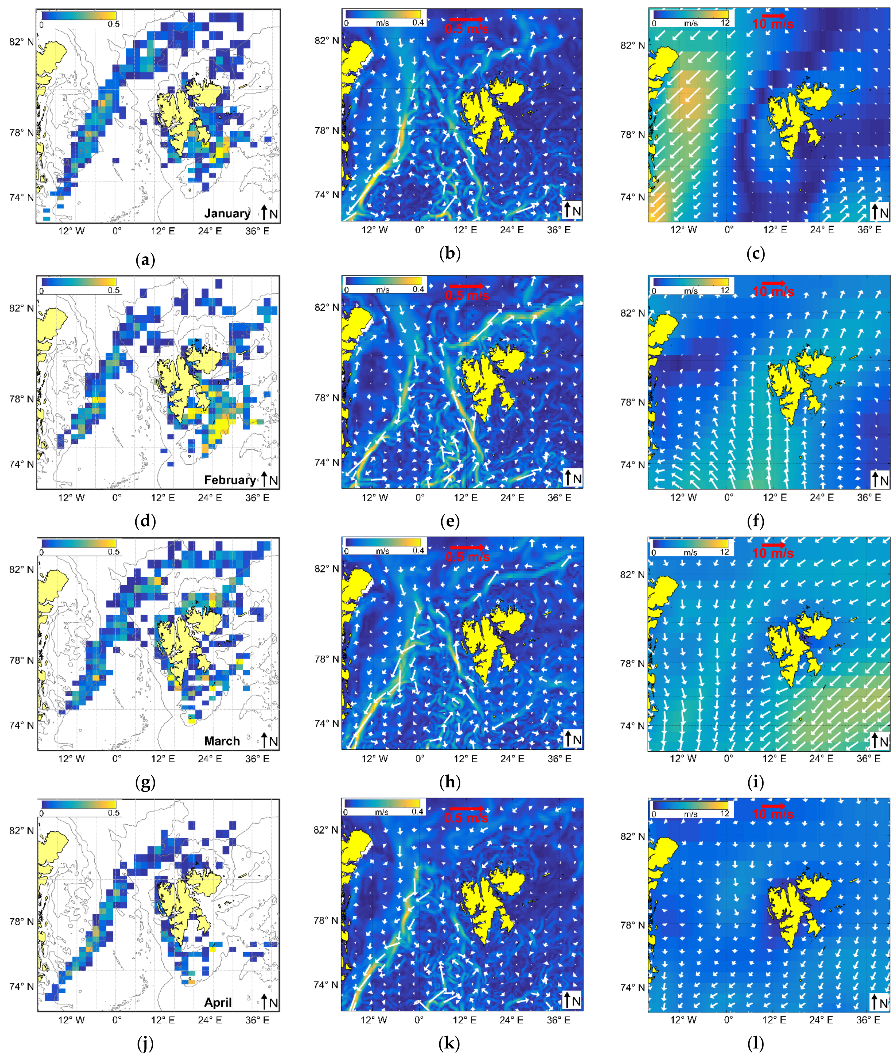
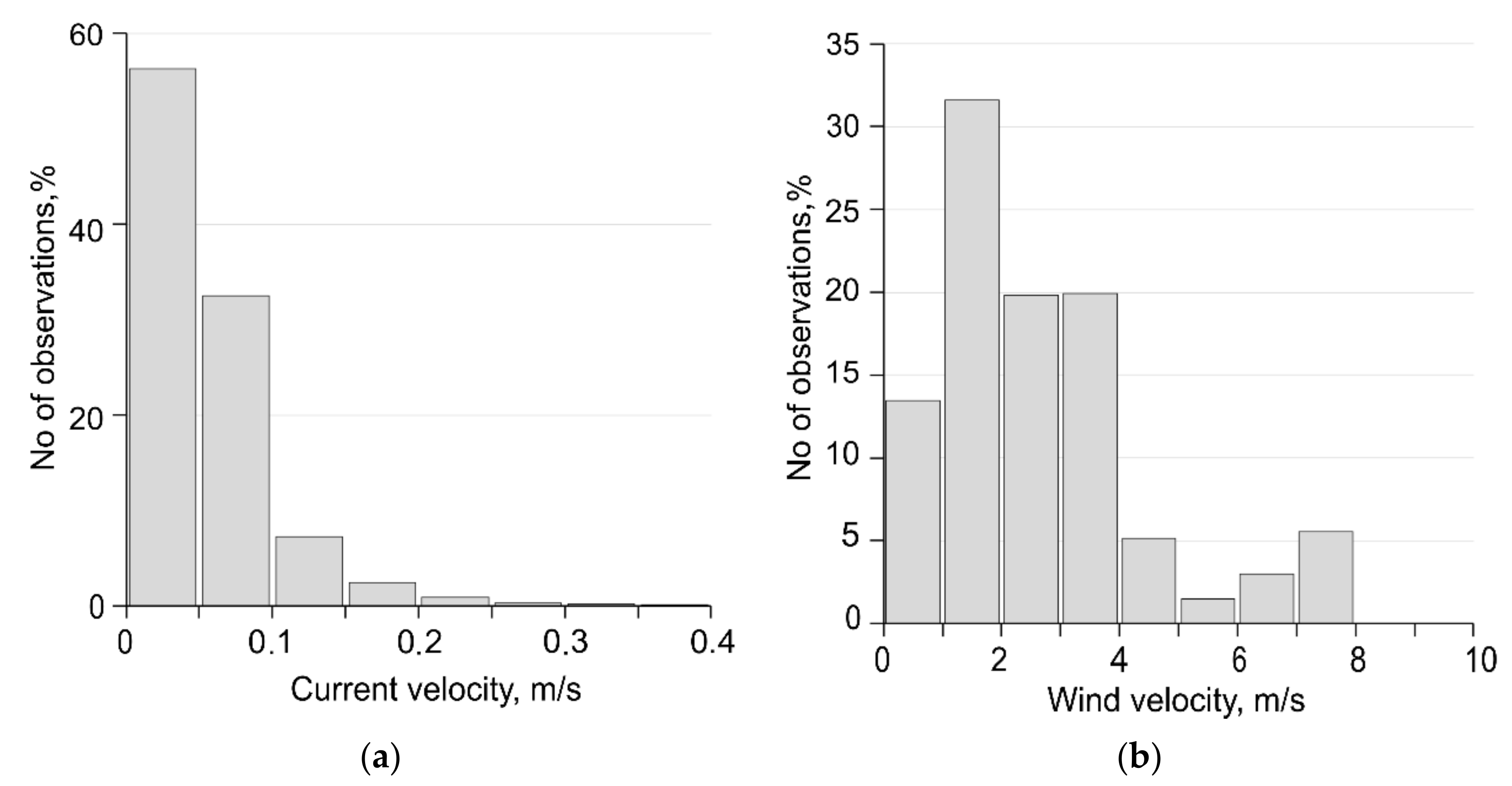
3.3. Relation to Boundary Currents and Winds

As seen from Figure 1 and Figure 5, bands of MIZ eddies are often found along or in close proximity to the main boundary currents of the region, i.e., the EGC, the WSC and its Svalbard and Yermak Branches, that follow topography and, in some locations, coincide with the ice edge boundary. In such case it seems reasonable to expect that intensity of boundary currents should have an impact on eddy generation at the ice edge and in the MIZ [1] as the eddy kinetic energy is highest along main currents over topography slopes [13]. Wind speed and direction are also key factors defining the movement of ice floes in the MIZ and resulting eddy generation [17,18,37].

To check the spatial correlation between eddies, currents and winds we have plotted monthly-mean distributions of these properties for January–April 2018 (Figure 10). The numbers of eddy detections between January and March are very similar (Table 2), but their probability maps have certain spatial differences (Figure 10, left column). The Fram eddy band between 74°–80° N is the most stable one and directly correlates with the position of main jet of the EGC directed southward (Figure 10a,b).

According to the GLORYS12V1 reanalysis data, the EGC intensity is highest in January, reaching 0.3–0.4 m/s (Figure 10b). At this time the Fram eddy band has high probability values and across-band width (Figure 10a). A monthly-mean wind field map shows a presence of northeasterly winds of 7–9 m/s over the Greenland Sea and western FS, and low winds of changing direction around Svalbard (Figure 10c). As seen from Figure 10a,c, high eddy probabilities over the Fram band are observed under moderate northeasterly winds that are favorable for eddy development at the ice edge in this region [18].

In turn, the eddy band north of 80° N (at 0–40° E, hereinafter, northern band) have largest area but moderate probability values that also correspond to moderate intensity of background currents (Figure 10b). As seen, the eddy activity is higher in the western part of the band influenced by northeasterly winds that blow parallel to the ice edge causing a westward movement of sea ice and upwelling along the ice edge. Lastly, rather intense eddy generation is observed near Hopen Island, where both currents and winds seem to be rather weak.

In February 2018, when the maximum number of eddies is registered, the WSC Svalbard Branch is intensified, but the eddy band is patchy and locates north of the main current. We do not see more eddies forming in this region. Instead, eddy probability has a maximum southeast from Hopen Island, where the currents are slightly more intense compared to January (Figure 10e). The wind field map shows a pattern of enhanced southerly winds that appear to favor eddy formation in FS and near Hopen.

In March 2018, the northern band has high probability values with the highest one registered over the southeastern slope of YP (Figure 10g), where currents are rather intense (Figure 10h). The wind speed is also relatively high and of favorable northern–northeastern direction. Further hot spots of eddy generation/observations are forming just north of North East Land (see Figure 1) and along the southwestern coast of Spitsbergen. Enhanced currents and 7–9 m/s northeasterly winds are seen over Hopen Island, but no apparent rise in eddy probabilities is seen in this case.

In April 2018, the overall intensities of the boundary currents and winds are lowest that, in general, correlates quite well with the smallest number of detected eddies and the lowest eddy probabilities apart of the Fram band (74–80° N) where the intensities of currents and eddies are still quite pronounced. The northern band shifts closer to Svalbard with no peaks in eddy probabilities, in agreement with weak currents in this region.

To sum up a general correspondence of eddies to background currents and winds, Figure 11 shows histogram distributions of the number of eddies observed in winter 2018 as a function of background current velocity and wind speed. Though there is a certain portion of eddies observed over the regions with enhanced currents of 0.2–0.4 m/s, most of them were observed in the regions with modest current velocity below 0.1 m/s (Figure 11a). As for the wind speed, most of the detected eddies were observed over low winds of 1–4 m/s, while about 15% of eddy observations were made under moderate winds of 4–8 m/s (Figure 11b).

4. Discussion

Here we should make a remark about the reported eddy numbers, their changes from month to month, and the spatial maps of eddy probability. The typical lifetime of eddies generated at the ice edge or inside the MIZ could be from couple of days to couple of weeks. In such case almost every eddy (apart of very short-lived ones) in the record would be repeatedly identified in SAR images. Surely, the most accurate counting of MIZ eddies would need a precise tracking of every individual eddy whose surface/SAR signatures may strongly evolve throughout its lifetime. This is a difficult and a time-consuming task. To simplify it, we have applied a simple normalization of the total number of detected eddies by the SAR coverage. This allowed to answer two simple, yet very important questions—when and where the number of detected eddies, assumed to be proportional to their generation intensity, was highest over the study region during these two particular winter seasons.

As already mentioned above, the winter seasons of 2007 and 2018 were selected arbitrary. However, both these years were characterized by anomalous states in regard of sea ice and hydrographic conditions, e.g., the year of 2007 was known as one of the years with record minimum ice extent in the Arctic Ocean, while the year of 2018 had an anomalously low sea ice outflow through Fram Strait [38,39] and rather long MIZ. Without going into details, it is obvious that the results from these two years might not apply in all years. Specifically, the zonal position/extent of the main eddy bands, i.e., the Fram band, the northern band and near Hopen are different in 2007 and 2018, and might differ with those in other years.

The obtained results clearly show that submesoscale and small mesoscale eddies dominate in the record, while the overall range of eddy diameters spans from 1 km to 68 km. Both cyclones and anticyclones have a peak in the range of diameters of 1–10 km. At diameter scales of 1–15 km, cyclones strongly dominate over anticyclones, in agreement with historical field observations [1] and model results [8]. However, in the range of 15–30 km this difference is gradually vanishing, and for diameter values above 30 km we observe an approximate parity between them, in agreement with satellite altimetry results [24,40], with a slight dominance of anticyclones. Such a transitioning from dominating cyclones to anticyclones happens when the eddy size exceeds the Rossby deformation radius, i.e., when mesoscale eddies start to dominate over submesoscale, as earlier reported for open-ocean eddies in [22,30]. However, to our knowledge, such a peculiarity has never been reported before for the MIZ eddies.

Another notion should be completed regarding the specifics of SAR imaging of eddy features of certain spatial scales. For the ice-free regions, SAR observations are known to have a certain bias toward relatively small, predominantly submesoscale eddies often having pronounced surface patterns due to more intense convergence zones at the surface as compared to mesoscale eddies. Such signatures strongly depend on background winds and are well-detectable under low to moderate wind conditions [41]. In this case spatially varying oceanic and atmospheric conditions add complexity for identifying large eddy structures over open ocean. However, within MIZ and at the ice edge, where floating ice serves as a tracer, the visibility of eddy signatures in SAR is not limited by winds what allows the detection of large eddies as well (see examples e.g., in [1,4,7,23]). Therefore, we presume that our record should not have a pronounced bias toward small-scale eddies.

However, the observed dominance of cyclones at submesoscales might have a certain explanation that is linked to ice trapping by eddies. Using physical arguments, the model study [8] shows that the sea ice accumulates preferentially in submesoscale cyclones where the frictional Ekman pumping generates strong convergence, while anticyclones repel the sea ice. This fact is also supported by our results, though the observed difference in the amount of ice trapped by cyclones and anticyclones is not large. As a result, cyclones appear to have more pronounced ice-related surface signatures and, hence, are more easily identified in SAR data. Yet, the method of visual assessment of ice fraction in eddies used here is not very precise and can have certain errors. Therefore, future studies should address this question using automated machine learning methods (e.g., [42,43]) for sea ice detection and masking inside eddy patterns.

Here we also attempted to give a first-order estimate of the eddy-induced horizontal sea ice retreat using observed values of eddy radii and amount of sea ice trapped in the eddies, and empirical mean values of ice bottom ablation and ice thickness. The obtained average horizontal ice retreat is about 0.2–0.5 km·d^–1 ± 0.02 km·d^–1. These values are several times smaller than those obtained by Johannessen et al. [1] and Bondevik [18] which is mainly due to the lower mean eddy radii observed in our data and used for calculations. In our calculations, we discarded the effect of lateral ablation though it might be important for relatively small ice floes dominating in the MIZ [1]. Moreover, we presumed the equal role of cyclones and anticyclones in sea ice melt, while the latter are thought to be more efficient in ice melting due to Ekman upwelling caused by ‘Eddy Ice Pumping’ mechanism prominent within the compact ice zone [44].

The spatial patterns of the eddy-induced horizontal sea ice retreat derived from SAR data suggest a pronounced decrease in MIZ area and a shift in the edge location that does not contradict the observations. Though the obtained values have many uncertainties that should be carefully examined in a more thorough study, presented methodology allows to obtain first-order bulk estimates of eddy influence on sea ice melt in the MIZ.

The analysis of the spatial correlation between eddies, currents and winds shows that the intensity of eddy generation/observations and their detectability in the MIZ, and the width of eddy bands correlate with the intensity of northern and northeasterly winds, as also previously shown in [18]. In some regions, e.g., along the Greenland Sea shelf break, in Fram Strait and over the Spitsbergen Bank the probability values of eddy occurrence in the MIZ seem to correlate with stronger boundary currents, while north of Svalbard and over Yermak Plateau higher probability values are observed under low/moderate currents and winds.

5. Conclusions

In this work, we have attempted to document the generation/occurrence hot spots and properties of MIZ eddies in FS and around Svalbard from the analysis of distinct quasi-circular features seen in spaceborne SAR images. We believe that these features in the sea ice distribution are most likely caused by mesoscale and submesoscale eddies in the ocean below, as numerous previous studies confirm. However, there may be plenty more eddies further away from the ice or into the denser pack ice that do not lead to similar signatures well-detectable in SAR data. There can also be eddies that are mostly or entirely subsurface and, therefore, do not have a strong surface expression. Additionally, there may be non-circular features such as narrow filaments that are not considered here. In this sense our SAR-based results present only a lower limit of the real eddy activity occurring in the MIZ.

Open-ocean eddies were also detected in the used SAR data; however, their number was surprisingly small as compared to the summer season when an order of magnitude more eddies were detected (e.g., [16,23,24,25]). We link this to the less pronounced vertical stratification and the relatively high winds in winter season limiting eddy manifestation in SAR images. Therefore, our current study does not allow us to conclude whether the eddy generation intensity over the open-ocean regions is higher in winter as compared to summer, as models suggest (e.g., [11,12,14]).

Analysis of SAR data from historical Envisat ASAR and contemporary Sentinel-1 SAR-C missions clearly shows a better performance of the latter in terms of spatial coverage of the study site that allowed a broader identification of eddy generation/occurrence hot spots in the marginal ice zone. Two Sentinel-1 sensors allowed to identify 1.2 times more eddies than ASAR when normalized on the number of available SAR images. However, when accounting for 1.2 times longer MIZ in winter 2018 compared to winter 2007, the average number of eddies detected per one image per kilometer of MIZ length is similar in both years and does not depend much on the sensor used.

Almost twice better spatial resolution of Sentinel-1 means that it may better resolve spatial patterns of fine- and small-scale dynamic features in the MIZ. The orbital design of two Sentinel-1 sensors allows sequential mapping of MIZ eddies on a daily regular basis which is critical to assess their dynamic properties and evolution [7], that was previously available only from altimetry observations of large mesoscale open-ocean eddies in the Arctic Ocean [24,40]. However, in this study, we do not consider kinematic properties of MIZ eddies which is a subject of future work.

References

1. Johannessen, J.A.; Johannessen, O.M.; Svendsen, E.; Shuchman, R.; Manley, T.; Campbell, W.J.; Josberger, E.G.; Sandven, S.; Gascard, J.C.; Olaussen, T.; et al. Mesoscale eddies in the Fram Strait marginal ice zone during the 1983 and 1984 Marginal Ice Zone Experiments. J. Geophys. Res. Oceans 1987, 92, 6754–6772. [Google Scholar] [CrossRef] [Green Version]
2. Johannessen, O.M.; Johannessen, J.A.; Svendsen, E.; Shuchman, R.A.; Campbell, W.J.; Josberger, E. Ice-edge eddies in the Fram Strait marginal ice zone. Science 1987, 236, 427. [Google Scholar] [CrossRef]
3. Shuchman, R.A.; Johannessen, O.M.; Campbell, W.J.; Lannelongue, N.; Burns, B.A.; Josberger, E.G.; Manley, T. Remote sensing of the Fram Strait marginal ice zone. Science 1987, 236, 427–439. [Google Scholar] [CrossRef]
4. Wadhams, P.; Squire, V.A. An ice-water vortex at the edge of the East Greenland Current. J. Geophys. Res. 1983, 88, 2770–2780. [Google Scholar] [CrossRef]
5. Biddle, L.C.; Swart, S. The observed seasonal cycle of submesoscale processes in the Antarctic marginal ice zone. J. Geophys. Res. Oceans 2020, 125, e2019JC015587. [Google Scholar] [CrossRef]
6. Brenner, S.; Rainville, L.; Thomson, J.; Lee, C. The evolution of a shallow front in the Arctic marginal ice zone. Elem. Sci. Anth. 2020, 8, 17. [Google Scholar] [CrossRef]
7. Kozlov, I.E.; Plotnikov, E.V.; Manucharyan, G.E. Brief Communication: Mesoscale and submesoscale dynamics in the marginal ice zone from sequential synthetic aperture radar observations. Cryosphere 2020, 14, 2941–2947. [Google Scholar] [CrossRef]
8. Manucharyan, G.E.; Thompson, A.F. Submesoscale sea ice–ocean interactions in marginal ice zones. J. Geophys. Res. Oceans 2017, 122, 9455–9475. [Google Scholar] [CrossRef]
9. Swart, S.; du Plessis, M.D.; Thompson, A.F.; Biddle, L.C.; Giddy, I.; Linders, T.; Mohrmann, M.; Nicholson, S.-A. Submesoscale fronts in the Antarctic marginal ice zone and their response to wind forcing. Geophys. Res. Lett. 2020, 47, e2019GL086649. [Google Scholar] [CrossRef] [Green Version]
10. von Appen, W.J.; Wekerle, C.; Hehemann, L.; Schourup-Kristensen, V.; Konrad, C.; Iversen, M.H. Observations of a submesoscale cyclonic filament in the marginal ice zone. Geophys. Res. Lett. 2018, 45, 6141–6149. [Google Scholar] [CrossRef]
11. Crews, L.; Sundfjord, A.; Albretsen, J.; Hattermann, T. Mesoscale eddy activity and transport in the Atlantic Water inflow region north of Svalbard. J. Geophys. Res. Oceans 2018, 123, 201–215. [Google Scholar] [CrossRef] [Green Version]
12. Hattermann, T.; Isachsen, P.E.; von Appen, W.-J.; Albretsen, J.; Sundfjord, A. Eddy-driven recirculation of Atlantic Water in Fram Strait. Geophys. Res. Lett. 2016, 43, 3406–3414. [Google Scholar] [CrossRef] [Green Version]
13. Wang, Q.; Koldunov, N.V.; Danilov, S.; Sidorenko, D.; Wekerle, C.; Scholz, P.; Bashmachnikov, I.L.; Jung, T. Eddy kinetic energy in the Arctic Ocean from a global simulation with a 1-km Arctic. Geophys. Res. Lett. 2020, 47, e2020GL088550. [Google Scholar] [CrossRef]
14. Wekerle, C.; Wang, Q.; Von Appen, W.-J.; Danilov, S.; Schourup-Kristensen, V.; Jung, T. Eddy-resolving simulation of the Atlantic water circulation in the Fram Strait with focus on the seasonal cycle. J. Geophys. Res. Oceans 2017, 122, 8385–8405. [Google Scholar] [CrossRef]
15. Wekerle, C.; Hattermann, T.; Wang, Q.; Crews, L.; von Appen, W.-J.; Danilov, S. Properties and dynamics of mesoscale eddies in Fram Strait from a comparison between two high-resolution ocean–sea ice models. Ocean Sci. 2020, 16, 1225–1246. [Google Scholar] [CrossRef]
16. Atadzhanova, O.A.; Zimin, A.V.; Romanenkov, D.A.; Kozlov, I.E. Satellite radar observations of small eddies in the White, Barents and Kara Seas. Phys. Oceanogr. 2017, 2, 75–83. [Google Scholar] [CrossRef] [Green Version]
17. Cole, S.T.; Toole, J.M.; Lele, R.; Timmermans, M.; Gallaher, S.G.; Stanton, T.P.; Shaw, W.J.; Hwang, B.; Maksym, T.; Wilkinson, J.P.; et al. Ice and ocean velocity in the Arctic marginal ice zone: Ice roughness and momentum transfer. Elem. Sci. Anth. 2017, 5, 55. [Google Scholar] [CrossRef] [Green Version]
18. Bondevik, E. Studies of Eddies in the Marginal Ice Zone along the East Greenland Current Using Spaceborne Synthetic Aperture Radar (SAR). Master’s Thesis, The University of Bergen, Bergen, Norway, 2011; 95p. [Google Scholar]
19. von Appen, W.J.V.; Schauer, U.; Hattermann, T.; Beszczynska-Möller, A. Seasonal cycle of mesoscale instability of the West Spitsbergen Current. J. Phys. Oceanogr. 2016, 46, 1231–1254. [Google Scholar] [CrossRef] [Green Version]
20. Dokken, S.T.; Wahl, T. Observations of Spiral Eddies along the Norwegian Coast in ERS SAR Image; Rep. 96/01463; Norwegian Defence Research Establishment (NDRE): Kjeller, Norway, 1996; 29p. [Google Scholar]
21. Karimova, S.S. Spiral eddies in the Baltic, Black and Caspian seas as seen by satellite radar data. Adv. Space Res. 2012, 50, 1107–1124. [Google Scholar] [CrossRef]
22. Stuhlmacher, A.; Gade, M. Statistical Analyses of Eddies in the Western Mediterranean Sea based on Synthetic Aperture Radar Imagery. Remote Sens. Environ. 2020, 250, 112023. [Google Scholar] [CrossRef]
23. Kozlov, I.E.; Artamonova, A.V.; Manucharyan, G.E.; Kubryakov, A.A. Eddies in the Western Arctic Ocean from spaceborne SAR observations over open ocean and marginal ice zones. J. Geophys. Res. Oceans 2019, 124, 6601–6616. [Google Scholar] [CrossRef] [Green Version]
24. Bashmachnikov, I.L.; Kozlov, I.E.; Petrenko, L.A.; Glock, N.I.; Wekerle, C. Eddies in the North Greenland Sea and Fram Strait from satellite altimetry, SAR and high-resolution model data. J. Geophys. Res. Oceans 2020, 125, e2019JC015832. [Google Scholar] [CrossRef]
25. Petrenko, L.A.; Kozlov, I.E. Properties of eddies near Svalbard and in Fram Strait from spaceborne SAR observations in summer. Sovr. Probl. DZZ Kosm. 2020, 17, 167–177. [Google Scholar] [CrossRef]
26. Kozlov, I.E.; Kudryavtsev, V.N.; Zubkova, E.V.; Zimin, A.V.; Chapron, B. Characteristics of short-period internal waves in the Kara Sea inferred from satellite SAR data. Izv. Atmos. Ocean. Phys. 2015, 58, 1073–1087. [Google Scholar] [CrossRef]
27. Lee, J.-S. Digital image smoothing and the sigma filter. Comput. Gr. Image Process. 1983, 24, 255–269. [Google Scholar] [CrossRef]
28. Spreen, G.; Kaleschke, L.; Heygster, G. Sea ice remote sensing using AMSR-E 89 GHz channels. J. Geophys. Res. Oceans 2008, 113, 1–14. [Google Scholar] [CrossRef] [Green Version]
29. Jakobsson, M.; Mayer, L.; Coakley, B.; Dowdeswell, J.A.; Forbes, B.; Fridman, S.; Hodnesdal, H.; Noormets, R.; Pedersen, R.; Rebesco, M. The International Bathymetric Chart of the Arctic Ocean (IBCAO) Version 3.0. Geophys. Res. Lett. 2012, 39, 1–6. [Google Scholar] [CrossRef] [Green Version]
30. Karimova, S. Observations of asymmetric turbulent stirring in inner and marginal seas using satellite imagery. Intern. J. Remote Sens. 2017, 38, 1642–1664. [Google Scholar] [CrossRef]
31. Fer, I.; Drinkwater, K. Mixing in the Barents Sea polar front near hopen in spring. J. Mar. Syst. 2014, 130, 206–218. [Google Scholar] [CrossRef]
32. Marchenko, A.V.; Morozov, E.G.; Kozlov, I.E.; Frey, D.I. High-amplitude internal waves southeast of Spitsbergen. Cont. Shelf Res. 2021, 227, 104523. [Google Scholar] [CrossRef]
33. Zatsepin, A.; Kubryakov, A.; Aleskerova, A.; Elkin, D.; Kukleva, O. Physical mechanisms of submesoscale eddies generation: Evidences from laboratory modeling and satellite data in the Black Sea. Ocean Dyn. 2019, 69, 253–266. [Google Scholar] [CrossRef]
34. Nurser, A.J.G.; Bacon, S. The Rossby radius in the Arctic Ocean. Ocean Sci. 2014, 10, 967–975. [Google Scholar] [CrossRef] [Green Version]
35. Kubryakov, A.; Stanichny, S.V. Mesoscale eddies in the Black Sea from satellite altimetry data. Oceanology 2015, 55, 56–67. [Google Scholar] [CrossRef]
36. Josberger, E.G. Bottom ablation and heat transfer coefficients from the 1983 Marginal Ice Zone Experiments. J. Geophys. Res. 1987, 92, 7012–7016. [Google Scholar] [CrossRef]
37. McPhee, M.G.; Maykut, G.A.; Morison, J.H. Dynamics and thermodynamics of the ice/upper ocean system in the marginal ice zone of the Greenland Sea. J. Geophys. Res. 1987, 92, 701–77031. [Google Scholar] [CrossRef]
38. Mayot, N.; Matrai, P.A.; Arjona, A.; Bélanger, S.; Marchese, C.; Jaegler, T.; Ardyna, M.; Steele, M. Springtime export of Arctic sea ice influences phytoplankton production in the Greenland Sea. J. Geophys. Res. Oceans 2020, 125, e2019JC015799. [Google Scholar] [CrossRef]
39. Sumata, H.; de Steur, L.; Gerland, S.; Divine, D.; Pavlova, O. Unprecedented decline of Arctic sea ice outflow in 2018. Res. Square 2021, 1–34. [Google Scholar] [CrossRef]
40. Kubryakov, A.A.; Kozlov, I.E.; Manucharyan, G.E. Large mesoscale eddies in the Western Arctic Ocean from satellite altimetry measurements. J. Geophys. Res. Oceans 2021, 126, e2020JC016670. [Google Scholar] [CrossRef]
41. Karimova, S.S.; Gade, M. Improved statistics of sub-mesoscale eddies in the Baltic Sea retrieved from SAR imagery. Int. J. Rem. Sens. 2016, 37, 2394–2414. [Google Scholar] [CrossRef]
42. Boulze, H.; Korosov, A.; Brajard, J. Classification of Sea Ice Types in Sentinel-1 SAR Data Using Convolutional Neural Networks. Remote Sens. 2020, 12, 2165. [Google Scholar] [CrossRef]
43. Park, J.-W.; Korosov, A.A.; Babiker, M.; Won, J.-S.; Hansen, M.W.; Kim, H.-C. Classification of sea ice types in Sentinel-1 synthetic aperture radar images. Cryosphere 2020, 14, 2629–2645. [Google Scholar] [CrossRef]
44. Gupta, M.; Marshall, J.; Song, H.; Campin, J.-M.; Meneghello, G. Sea-ice melt driven by ice-ocean stresses on the mesoscale. J. Geophys. Res. Oceans 2020, 125, e2020JC016404. [Google Scholar] [CrossRef]
Figure 1. Bathymetry map of study site showing schematic of main currents in Fram Strait and near Svalbard. Arrows indicate the directions of currents: WSC—West Spitsbergen Current, EGC—East Greenland Current, SB—Svalbard Branch, YB—Yermak Branch. Gray lines mark 200 and 2000 m isobaths.
Remotesensing 14 00134 g001
Figure 2. Spatial coverage of the study site by SAR data during: (a) December 2006–March 2007; (b) January–April 2018. The number of available SAR images is shown in color. The white line denotes the boundary of a region where the number of SAR images is below 10. Overlaid grey lines are the 200- and 2000-m isobaths taken from IBCAO v.3.0. Red dashed lines show the season-mean position of ice-water boundary for particular winter season.
Remotesensing 14 00134 g002
Figure 3. Map of normalized radar cross section showing an example of MIZ eddy manifestations in Envisat ASAR image acquired on 23 February 2007 at 12:17 UTC over Fram Strait. Notions given in different colors show position of consolidated ice (blue), MIZ (yellow) and open water (red).
Remotesensing 14 00134 g003
Figure 4. (a) Monthly variability of the normalized number of MIZ eddies detected in winter 2018; (b) histogram distributions of the number of eddies as a function of eddy diameter. Black and grey colors correspond to cyclones and anticyclones, respectively.
Remotesensing 14 00134 g004
Figure 5. Locations (a,b) and probability (c,d) of the MIZ eddies identified in spaceborne SAR data during winter of 2007 (a,c) and 2018 (b,d). Blue (red) circles in (a,b) mark cyclonic (anticyclonic) eddies. The thick white line in (a,b) denotes the boundary of a region with the number of SAR images below 10. Grey lines are the 500- and 2000-m isobaths.
Remotesensing 14 00134 g005
Figure 6. Spatial distribution of the mean (a,b) and the maximum (c,d) diameters of the MIZ eddies in 2006/2007 (a,c) and 2018 (b,d) in kilometers. Overlaid grey lines are the 200- and 2000-m isobaths.
Remotesensing 14 00134 g006
Figure 7. Histogram distributions of the number of eddies and their mean diameters observed in winter 2007 and 2018 as a function of: (a) depth corresponding to eddy locations; (b) sea ice concentration. Black and grey colors correspond to cyclones and anticyclones, respectively.
Remotesensing 14 00134 g007
Figure 8. Histogram distribution of sea ice fraction in eddies detected in Sentinel-1 SAR images in January 2018. Black (gray) bars indicate cyclonic (anticyclonic) eddies.
Remotesensing 14 00134 g008
Figure 9. Spatial distributions of: (a) ice fraction in eddies and (b) eddy radii in January 2018; the average horizontal retreat of the ice edge due to MIZ eddies for (c) January 2018 calculated using the data from (a,b); (d) for the entire winter 2018, when only r variations in space (shown in Figure 6b) were considered. Red, pink and green lines in (c) show the ice edge location from AMSR-2 data in the beginning (5th), middle (15th) and end (25th) of January 2018.
Remotesensing 14 00134 g009
Figure 10. Monthly-mean spatial fields of eddy probability in the MIZ (a,d,g,j), surface current speed [m/s] and direction from GLORYS12V1 reanalysis (b,e,h,k), and 10 m wind speed [m/s] and direction from ERA Interim Reanalysis (c,f,i,l) for January–April 2018. Red arrows show velocity scales in the middle and right columns. Overlaid grey lines in left column are the 200- and 2000-m isobaths.
Remotesensing 14 00134 g010
Figure 11. Histogram distributions of the number of eddies observed in winter 2018 as a function of (a) current and (b) wind velocities [m/s] around the locations of detected eddies derived from GLORYS12V1 model and ERA Interim Reanalysis.
Remotesensing 14 00134 g011