Dynamic Relationship Study between the Observed Seismicity and Spatiotemporal Pattern of Lineament Changes in Palghar, North Maharashtra (India)

Abstract

The Palghar region (north Maharashtra, India), located in the northwestern part of the stable continental region of India, experienced a low magnitude earthquake swarm, which was initiated in September 2018 and is continuing to date (as of October 2021). From December 2018 to December 2020, ~5000 earthquakes with magnitudes from M1.2 to M3.8 occurred in a small region of 20 × 10 km². These earthquakes were probably triggered by fluid migration during seasonal rainfall. In this study, we have used multi-temporal Landsat satellite data of the year 2000, 2015, 2018, 2019, and 2020, extracted lineaments, and studied the changes in frequency and pattern of lineaments before and after the initiation of the swarm in the Palghar region. An increase in the lineament density and amount of rainfall are found to be associated with the increasing frequency of earthquakes.

1. Introduction

The earthquakes in the Indian shield are common, in the past numerous small to large earthquakes have occurred in many parts [1,2,3,4,5,6,7]. These earthquakes occur along well-known lineaments and faults. Some of the earthquakes that occurred in the Indian shield are associated with reservoir seismicity (e.g., [4,8,9,10,11,12,13,14,15,16,17,18,19,20]). The Indian shield experienced several significant intraplate earthquakes [4,17,21,22,23,24,25,26,27,28,29,30,31,32,33,34,35,36,37,38,39]. Earthquake swarm (clustering of earthquakes) activities in time and space are common and observed in many parts of the country [40,41,42,43,44,45,46]. Earthquake swarms are triggered either due to a nearby large magnitude earthquake or due to the movement of water through fracture (weak) zones [42,43]. Generally, earthquake swarms are small in magnitude but sometimes they could lead to a large magnitude earthquake. A few places in western India, south Gujarat [41,43,44,45,46,47,48], and Saurashtra regions have earlier witnessed swarm-type earthquakes [42,43,49,50,51]. These events were attributed to triggering due to rainfall during the monsoon season [43,44,45,46,47]. On 3 March 2020, the swarms have attracted the attention of people living locally and in other regions of India, where efforts were made to clarify that the observed earthquakes may not lead to a big earthquake in the region [52]. Further, it was expressed that the earthquakes swarms observed on the west coast of India, could be due to tidal waves that may cause changes in the hydrological regime of the swarm regions [52]. Further, the ongoing swarm’s induced earthquakes were observed in the Palghar area [44] associated with energy in the high-frequency range (20–40 Hz) (audible range) is being monitored by many premier seismological institutions of India (e.g., National Centre for Seismology, Ministry of Earth Sciences, New Delhi and National Geophysical Research Institute, Hyderabad) using their own local seismic network. This has been later confirmed by the local residents who witnessed subterranean sounds like those generated due to blasting, in the epicentral region [53].

On 18 November 2018, unusual earthquake activities started in the Palghar District, Maharashtra located in the Deccan Volcanic Province of Western India [44,45] with the occurrence of an M3.8 earthquake on 11 November 2018. Among these, several events with magnitude ≥3.0 were also felt by the people in the Palghar area. The earthquakes of magnitude less than M2.0 were also recorded by the local seismographs, which may not be felt by the residents. These earthquakes occur in a tight cluster at shallow depths <10.0 km. Many of these events were also reported to be accompanied by audible sounds with or without shaking. The earthquake catalog of the Palghar region indicates that the region has not witnessed any major earthquake of magnitude >5.0 in the past few decades (see

Table A1. List of past earthquakes that occurred in the study area from 1702–2005.

SL. No.	Year	Month	Date	Latitude (°N)	Longitude (°E)	Depth (km)	Magnitude	Location	References
1	1702	-	-	19.700	73.100	-	3.7 Ms	Bhima river	CGS
2	1856	12	25	20.000	73.000	-	5.7 Ms	Near Dahanu	CGS
3	1856	12	25	20.000	72.99	-	5.7 Ms	Panvel region	CGS
4	1893	02	08	19.700	73.09	-	3.7 Ms	Bhima river	CGS
5	1935	07	20	20.000	73.000	-	5.0 Ms	Near Dumas	CGS
6	1935	07	20	20.000	72.999	-	5.0 Ms	Panvel region	CGS
7	1986	04	26	20.636	73.429	33	4.3 Ms	Near Surat	CGS
8	1986	04	28	20.712	73.367	33	4.3 Ms	Near Surat	CGS
9	1991	04	30	20.879	73.099	33	4.4 Ms	Near Surat	CGS
10	1998	11	17	19.490	73.261	-	2.9 Mc	Panvel region	Mohan et al., 2007; Bansal and Gupta, 1998
11	1999	06	30	19.981	72.767	25.8	3.0 Mc	Panvel region	Gupta et al., 1998; IRIS
12	1999	11	09	20.096	73.165	-	2.6 Mc	Panvel region	Mohan et al., 2007; Bansal and Gupta, 1998
13	2000	01	01	20.006	72.916	-	2.8 Mc	Panvel region	Mohan et al., 2007; Bansal and Gupta, 1998
14	2000	04	07	19.947	73.062	18	2.8 Mc	Panvel region	Mohan et al., 2007; Bansal and Gupta, 1998
15	2001	03	14	19.526	72.894	-	3.0 Mc	Panvel region	Mohan et al., 2007; Bansal and Gupta, 1998
16	2001	12	22	19.807	72.932	-	3.3 Mc	Panvel region	Mohan et al., 2007; Bansal and Gupta, 1998
17	2002	05	17	19.817	72.843	22.5	2.2 Mc	Panvel region	Gupta et al., 1998; IRIS
18	2002	10	1	19.496	73.024	8.3	2.7 Mc	Panvel region	Gupta et al., 1998; IRIS
19	2003	01	16	19.487	73.229	23.0	2.3 Mc	Panvel region	Gupta et al., 1998; IRIS
20	2003	05	12	18.469	73.035	20.1	3.3 Mc	Panvel region	Gupta et al., 1998; IRIS
21	2003	10	01	19.526	73.315	23.2	2.4 Mc	Panvel region	Gupta et al., 1998; IRIS
22	2005	10	15	20.090	73.127	-	3.3 Mc	Panvel region	Gupta et al., 1998; IRIS
23	2005	10	28	20.002	73.013	-	3.3 Mc	Panvel region	Gupta et al., 1998; IRIS
24	2005	10	28	20.069	73.185	-	3.3 Mc	Panvel region	Gupta et al., 1998; IRIS

Source: Historical earthquakes information taken from available published literature [34,67,68]; and ‘-’ means data not available. Note: Due to the large volume of the earthquake swarm points, the details of the catalog update till 31 December 2020 are not attached with this table. The swarms data are available to the user upon request. The detailed access request of the swarms catalog is given in the data availability statement section.

). In the present study, we have analyzed changes in density and pattern of tectonic lineaments using Landsat data of five years 2000, 2015, 2018, 2019, and 2020 before and after the beginning of the earthquake swarm in the Palghar region.

1.1. Earthquake Swarm in Palghar Region

The observed earthquake swarms including historical earthquakes in the Palghar region are shown in Figure 1. This region falls in seismic zone III in the seismic zoning map of India [54] where the intensity of VII or VIII from the regional large earthquakes or local earthquakes are expected. In the present study, we have closely examined the earthquake swarm activity in the region bounded by latitude 19.42°–20.93°N and longitude 72.40°–73.25°E (Figure 1, red bounding box). The Indian shield region is relatively more active and is made of different cratons, which have undergone significant deformation in geological time. The geomorphological and lineaments features are good indicators of neo-tectonics of any region. Tectonic lineaments derived from satellite data have been mapped by many in different parts of the world and contrast differences in the density of lineaments prior to and after earthquakes are reported [54,55,56,57,58,59,60,61,62,63]. Further, the need for lineament mapping has been stressed to evaluate seismic hazard zones and long-term earthquake forecasts.

In the present study, we considered Landsat satellite images for the years 2000, 2015, 2018, 2019, and 2020 to extract tectonic lineaments and soil moisture changes by applying soil moisture index (SMI) derived from the freely available archive of USGS earth explorer. To validate these changes, we further focused on some meteorological and geophysical parameters (rainfall, surface skin temperature, and soil moisture content at 0–10 cm depth) produced with the Giovanni online data system (https://giovanni.gsfc.nasa.gov/giovanni/#service, accessed on 3 November 2020) developed and maintained by the NASA’s Goddard Earth Sciences Data and Information Services Center (GES DISC) [64]. The parameters we considered to study changes in surface or sub-surface in the swarm regions at the surface or certain depth. As it is suggested that earthquakes were probably triggered by the fluid migration during seasonal rainfall [45], therefore, the above-mentioned meteorological and geophysical parameters were mainly selected to understand the seismicity in the study area. Moreover, this study helps us to understand the rainfall-induced earthquakes in the region.

1.2. Geological Settings and Geophysical Information of the Study Area

The source zone of the swarm activities in the Palghar region is covered with a thick fractured basaltic rock. In this study, the Palghar swarm covers an area of approximately 200 km² located within 10 km of the highway NH-8 [65], which is ~45 km north of Palghar, ~110 km north of Mumbai, and ~20 km east of the western coast of India (Figure 2). The study area is shown with the vertical red bounding box (Figure 2a), which consists of two major geological settings, Q refers to ‘Quaternary’ in the Navsari district area and TKv broadly represents the entire SW under ‘Cretaceous-Paleocene Volcanic’ origin [66] (Figure 2b). The earthquakes are located close to several regional faults such as the axis of Panvel flexure, N-S oriented normal fault known as ‘West Coast Fault’ (WCF, Figure 1), Neo-tectonic fault, several basement faults, and major lineaments (Figure 1c and Figure 2c).

The geophysical studies along the western continental margin of the Indian shield ascertained the thickness of the trap, crust, and lithosphere including the basement configuration [69,70,71,72,73,74]; Pavankumar and Manglik [75] delineated the upper crustal structure based on electrical conductivity. They advocated that the upper crustal heterogeneities are coupled with the basement fault and the low rheological strength of the fractured upper-to-middle crust might be leading to triggering of the seismicity in the region. The above idea has been also reported by Roy [76] that the heterogeneous deformation is comparable to block tectonics that restricts the relative movements of the Indian Shield. Therefore, internally the blocks remain rigid, which might trigger earthquake activities. Epicenters of all the known recorded major earthquakes lie either on major lineaments or reasonably close to them. Further, we made an effort to understand the influence of retrieved meteorological and geophysical parameters on lineaments and associated earthquake activities.

Based on the density and orientations of lineaments from satellite images in the last 20 years observed by us, the earthquake swarm activity and its relationship with the spatiotemporal pattern of lineament changes observed in this study are discussed. The observed seismicity revealed a complex phenomenon interplay within the earthquake swarm region and its surroundings, confirmed through meteorological and geophysical parameters and temporal lineaments changes.

2. Datasets and Methods

2.1. Data Used

The seismicity data were considered in this study from the catalog of the National Centre for Seismology (NCS) [www.seismo.gov.in (accessed on 3 November 2021)] and published literature [45]. The observed earthquake epicenters were clustered along the national highway (NH-8) and its close adjoining areas especially located between Dahanu and Talasari geographic areas (Figure 2b). It is mentioned that the earthquakes catalog used in this study, compiled by NCS. The NCS is monitoring ongoing earthquake activities by a temporary seismological network established on 12 December 2018. NGRI, Hyderabad is also monitoring ongoing earthquake activities since 30 January 2019. Here, we have considered the earthquake M ≥ 1.2 from December 2018 to December 2020 in the present study, the activities are further being monitored. In the study area, the earthquake swarm (M ≤ 3.5) is located close to the Kurze reservoir and a few villages where people experienced the swarm activities over a long period. In addition, past earthquakes datasets from 1702 AD to 2005 [34,67,68] were also collected from the earthquake catalog (1200 AD to 2005) of published literature, and there only selective earthquakes (24 in total) were considered in the study area.

We also made efforts to study the changes in lineaments derived from multi-temporal Landsat satellite images with path 148 and row 046, available from freely available USGS Earth explorer archive (https://earthexplorer.usgs.gov, accessed on 3 November 2020) [77]. To observe temporal lineaments changes, we have considered images under different scenarios such as, for past scenario Landsat–5 TM 2000 (16 January 2000), before earthquake swarm, Landsat–8 OLI for 2015 (9 January 2015), and 2018 (1 January 2018), 2019 (20 January 2019) for ongoing change referring to earthquake swarm activities, and 2020 (23 January 2020) for present scenario, respectively. Lineament density and orientation studies through rose diagram were found ideal to discuss in view of the earthquake swarm activities in an area. Lineament changes prior and after were observed immediately after the Bhuj 2001 earthquake [78] and two other different earthquakes such as Gorkha of Nepal (M7.9) in 2015 and Imphal of Manipur (M6.7) [79] were used in a single study for comparison only to observe the pattern of lineaments changes [79].

We have considered monthly average rainfall (mm), average surface skin temperature (kelvin), and soil moisture content (kg m⁻²) data from the NASA Giovanni portal (https://giovanni.gsfc.nasa.gov/giovanni/#service (accessed on 3 November 2021) [64]. These parameters have been selected as meteorological and geophysical parameters changes are observed by numerous studies focusing on induced seismicity in the fault regions where the majority of earthquakes are concentrated, and all changes are related to the surface. Therefore, we considered the rock fractured concept, as during the progress of earthquake event, high stress along the tectonic faults is observed and surface temperature increasing phenomena are observed before and after the earthquake events in several active fault areas in the world.

2.2. Methodology

2.2.1. Image Pre-Processing and Lineaments Extraction from Remote Sensing Data

In this study, we focused to monitor multi-temporal lineament changes in the wide swath areas of Landsat satellite imageries, where present earthquake swarms are located. These changes were observed in different time periods (2000, 2015, 2018, 2019, and 2020) to monitor the changes in lineaments and corresponding earthquake activities. We carried out pre-processing steps at the initial stage, from digital numbers (DN) to atmospherically corrected reflectance image conversion using the FLAASH (Fast Line-of-sight Atmospheric Analysis of Hypercubes) module in ENVI 5.3 software and applied linear 5% stretch over multispectral data to enhance better visualization. In the next, images were assigned to WGS 1984 datum with the projection parameter of UTM zone 46N.

Further, principal component analysis (PCA) was performed on each image, and PC1 best band selection was carried out based on Eigen number and Eigenvalue to utilize the image (grayscale) in automatic discontinuities structural lineaments extraction. This automatic extraction process is done by following the common popular traditional method i.e., the Line algorithm of PCI Geomatica software [79,80,81,82,83]. Various computer-aided methods such as edge detection, thresholding, and curve extraction steps were involved in the processes. For processing and extraction of lineaments, the following algorithm parameters and their user-defined corresponding values were assigned in the line algorithm window, such as RADI–Radius of the filter in pixels (10), GTHR–Threshold for edge gradient (50), LTHR–Threshold for Curve length in pixels (30), FTHR–Threshold for Line fitting error in pixels (3), ATHR–Threshold for Angular difference in degrees (15), and DTHR–Threshold for linking distance in pixels (20). The extracted raw lineament data saved as permanent vector polyline (shapefile) features, further imported and performed line splitting operation with a model builder in ArcGIS 10.8 software. Subsequently, with the help of road and railways features (taken from Geofabrik, OpenStreet Map data; http://download.geofabrik.de/asia.html; accessed on 10 June 2020) [65] checking were performed in extracted lineaments data derived from each satellite image to avoid the anthropogenic artifacts [78,79,81,82,83,84].

2.2.2. Lineament Density and Satellite Image Derived Soil Moisture Analysis

Based on the observed lineament after detailed processing, we have plotted lineament density with different classes using the quantile classification method of ArcGIS 10.8 software to understand the structural changes and surface stress pattern in the study area. In the final stage, the corrected lineament data shapefile is exported to AutoCAD dxf format to know its orientation, and this has been performed through a rose diagram generated using Rockworks Advanced 2018 (RockWare Inc., Golden, CO, USA) software. The number of lineaments, their density changes, and the statistical analyses are further carried out in the swarm region with the aid of ArcGIS 10.8 software. At this stage, the distribution of the changes in lineaments at the local level is compared with the broad regions. The descriptive statistics of the frequency of lineament and density changes at five-time domains are taken into account to relate with the lineaments and earthquake swarm activity in the study area.

In addition, the same Landsat atmospheric corrected reflectance images in five different times (e.g., 2000, 2015, 2018, 2019, and 2020) were considered to observe the Soil Moisture Content (SMC) of the broad study regions, further narrowly focused on earthquake swarm regions (red bounding box). This has been done by applying Soil Moisture Index (SMI) in each respective image with the given Equation (1) by Dupigny-Giroux et al. [85].

$$SMI=\frac{NIR}{VisBlue}$$

(1)

where, NIR is the near-infrared reflectance band 4 (0.77–0.90 µm); VisBlue reflectance is the visible blue band 1 (0.45–0.52 µm) for Landsat–5 TM and band 5 (0.85–0.88 µm) and band 2 (0.45–0.51 µm) for Landsat–8 OLI, respectively.

2.2.3. Earthquake 2D Depth and 3D Mesh Model, and Spatial Variations Analysis Method

In addition, earthquake focal depths were considered to generate a 2D depth map of the study regions by applying the Inverse Distance Weighted (IDW) interpolation method of utilizing spatial analyst extension of ArcGIS 10.8 software. IDW interpolation was used to visualize the number of earthquake occurrences at which depth, more specifically, to know the spatial details on how many of them are in shallow, intermediate, and deep-seated earthquakes. To prepare earthquake depth map, quantile classification method was used with 10 class ranges representing with brown (highest depth) to ocean blue (lowest depth) intensity color depth (see Section 3.5 for detailed discussion) and then grayscale tiff images are processed by ENVI 5.3 software to construct depth series profile. As indicated earlier in Figure 1 (top-bottom left) North-South and East-West directions are marked as a reference, where we constructed 8 transects across the image at different directions (4 are in N-S direction refers to VT (1–4) and 4 are in E-W direction refers to HT (1–4)). These transects are constructed using ENVI 5.3 software to observe the earthquake depth variations at a spatial scale. The corresponding depth profile pictures are based on pixels considered within the transect line, where depth info is automatically placed in the vertical bar as the data value. Further, based on all earthquake swarms, a 3D mesh model was generated to know spatial variations of the earthquake swarm events according to the reported occurrence depth level.

2.2.4. Meteorological and Geophysical Parameters Analysis Method

We have analyzed two meteorological and one geophysical parameter i.e., rainfall and monthly skin temperature, and soil moisture [86] to check whether these parameters have direct or indirect influences on the occurrences of earthquake swarm activity or not within the study region. The time-series area-averaged daily accumulated precipitation (combined microwave-IR) (GPM-3IMERGDE-V06) [86] with spatial resolution 0.10 was considered for monthly rainfall (mm) estimation. The monthly average surface skin temperature (unit: kelvin) with 0.5 × 0.625 degrees (MERRA–2 model M2TMN*SLV version 5.12.4) (Figure 8c) and monthly averaged time-series soil moisture content (unit: kg m⁻²) (0–10 cm underground) (GLDAS_NOAH025M v 2.1) model with 0.25° spatial resolution (Figure 8b) were saved in the similar time domain for the comparative analysis and its association with monthly total earthquakes of the earthquake swarm areas.

2.2.5. Observed Seismicity

We also considered historical and reported earthquakes distributions from 1702 AD to 2005 for the analysis. The recent earthquake activities are considered in the lineament density red bounding box (similar to Figure 1b,c) with geographic co-ordinate extension 19.42°–20.93°N and 72.40°–73.25°E. Additionally, we also explored the changes in lineaments associated with the surface manifestations in the north Maharashtra area and its relations with the observed seismicity. The lineament data are mapped using multiple Landsat images for the entire areas in different time periods.

From December 2018 to December 2020, a clustering of small magnitude earthquakes is observed in the Palghar region that we refer to as the Palghar earthquake swarm activity. The total earthquakes recorded by the temporary network of NCS is 29,330 of magnitude 1.1 to 3.8. However, about 5000 earthquakes of local magnitude M1.2–M3.8 were reported by NCS during December 2018 to December 2020. Out of these, 10% of earthquakes have M ≥ 3.0 and the first event of the maximum magnitude of M3.8 occurred on 01 March 2019. The ctivity in 2020 is following a trend similar to the one noticed during 2018–2019. The focal depths of the events are mostly depth <10 km, and the magnitude range is found to be M0.4 to 3.8 [45]. Most of the earthquakes (~90%) have magnitudes <2.0. The general trend of the present activity is along NNE—SSW directions and is located close to the two tectonic structures namely, Panvel flexure and WCF (Figure 1 and Figure 2c), which are mostly associated with the Deccan volcanism and tectonics in conformity with the strike of the local lineaments. The Palghar region has no instrumental record of seismicity but, earthquake swarms have been reported from adjacent locations within the same tectonic-geological setting. The lithology of the area is composed of the fractured rock mass of Deccan basalt, which may provide a favorable medium for rainwater to subsurface infiltration. Nevertheless, the area receives only monsoon rainfall and no clear connection between the rainfall and seismicity could be established due to limited data sets. Table A1 shows 24 reported earthquakes in and around the Palghar area. The study of magnitude-frequency relation of Gutenberg-Richter (1944): logN = a-bM, is considered in this study [87,88], where a, b values are constants. The distribution implies that the estimated magnitude of completeness in the catalog is 1.2 in the Palghar area (Figure 3), so we may consider magnitude greater or equal to 1.2 for any statistical analysis. The calculated Mc was found as 1.2 with a 90% goodness-of-fit level [89]. The estimated Mc assumes of a power-law Gutenberg–Richter relationship and the magnitude where the first derivative of the frequency–magnitude curve has its maximum is taken as the Mc value. Mc can also be defined as the lowest magnitude in which 100% of the events are detected in space and time volume [90].

Therefore, accurate knowledge of Mc is essential for many seismicity-based studies, particularly seismicity parameters such as the b-value of the G-R relationship. As such, a large b-value indicates a high frequency of earthquakes with relatively small magnitudes of earthquakes. The estimated b-value is 1.00 ± 0.01 in this study, which indicates that the earthquake occurred due to active tectonics in the region.

3. Results

3.1. Regional Seismicity Analysis

From 1702 AD to 2005 [34,67,68] seismic activities were sporadically distributed in the study area (see Table A1). In this study, we have considered 24 past earthquakes of magnitudes M2.4 to M5.7 taken from reported and available earthquake catalogs during 1200 AD–2005. Out of 24 earthquakes, 17 are located in the Panvel region, 3 are near to Surat, 2 others in the Bhima River (month date unclear, 1702) with M3.7 and near Dumas (occurred on 20 July 1935) with M5.0, and only one in near Dahanu occurred on 25 December 1856 [67] with M5.7 and the depth is unclear as reported by the Indian Meteorological Department (IMD). However, during 1986–1999, only M 2.6–4.5 earthquakes occurred and from 1 January 2000 to 28 October 2005 earthquakes of magnitudes M2.8–M3.3 occurred in the study areas. In an earthquake catalog, the magnitude of completeness is the minimum magnitude above, which all earthquakes within a certain region are reliably recorded. To get any reliable conclusions, it is recommended to check the completeness of the earthquake catalog. For example, in Gutenberg-Richter’s (G-R) 1954 [88] distribution of earthquake magnitude, it is expected that in a shorter time window there are fewer (even no one) earthquakes of large magnitudes occurred in any region. Therefore, this study progress with the G-R distribution of the earthquake swarms (Figure 3) from December 2018 to December 2020 to make a reliable earthquake catalog for the study area.

3.2. Observed Lineament, Temporal Changes and Density Measurement from 2000 to 2020

To observe the past lineaments (Figure 4), we commenced from the year 2000 and continue till 2015 (Figure 4a,b). According to Landsat–5 TM (2000) derived results, total lineaments observed 1508 in number (Figure 4a) immediate after the Mc 2.8 earthquake occurred on 1 December 2000 (see Table A1) and its orientation was in NE–SW and NNE–SSW trend with mean strike line (red color) position approx. 29° NE to 209° SW direction. During this time, the number of lineaments were observed low-medium as confirmed through extracted lineaments and lineament density values (LD_Max value 0.79 km/km²) (Figure 4b). From 1 December 2000 to 28 October 2005, 12 earthquakes occurred at shallow to deep-focus earthquakes (8–25 km depth), and we assumed that north Maharashtra suffered from surface manifestations representing shield areas were tectonically viable to generate more earthquakes afterward.

In 2015, changes in stress have been observed through lineaments data on 9 January 2015 (Figure 4c) almost 2.34 times increase in lineaments with mean strike line (red color) direction 47° NNE to 227° SSW along with medium-high stresses have been observed, which is represented with LD_max value 1.04 km/km² (Figure 4d) compared to 16 January 2000 (Figure 4b).

To continue with Palghar earthquake swarm activities, lineaments retrieved from the 1 January 2018 imagery (Figure 4e) show a similar trend to that in 2015, with the number of lineaments recorded at 1600 with an LD_Max value of 1.05 km/km² (Figure 4f). This indicates the presence of ongoing stresses in the broad regions including swarm regions which began in 2015 (9 January 2015 in our case) and the mean strike line (red color) position was in approximately NNE (N49°) to SSW (N229°) direction (average 2° forward rotating than 2015) along with medium-high stresses observed. The northern Maharashtra portion is a tectonically active region where we observed an increase in the lineaments up to 1600 in number on 1 January 2018 compared to 20 January 2019 (number of lineaments 961) (Figure 4g). Such changes in the number of lineaments are associated with the starting of earthquake swarms (Figure 4e), a sharp 1.72-fold decrease, with LD_Max value of 1.20 km/km² (Figure 4h) with mean strike line position was in approximately 47° NNE to 227° SSW direction (approximately 2° rotating back from the mean strike of 2018). During this time medium-high stresses were observed and change in stresses occurred as the lineaments dropped. Therefore, this could be occurred due to changes in surface deformation, and soil moisture content.

As we observed that the earthquake swarm is continuing, we have focused our lineament analysis using recent Landsat imagery of 23 January 2020 (Figure 4i), where lineament density is found to increase almost 2-fold (1845 lineaments) compared to 20 January 2019 (961 lineaments) with LD_Max value 1.19 km/km² (Figure 4h) and mean strike position advancing 2° rotating forward compared to 2019. However, in 20 years cycle (2000–2020), lineaments increase by 2.78-fold, with a mean strike position moving forward (approximately 16°) with the shifting of lineaments’ directions from NE-SW to NNE-SSW. The subsequent temporal lineament maps have been visually compared within ArcGIS 10.8 software and the change in lineaments direction is represented with the rose diagram incorporated as an inset image within individual figures (Figure 4a,c,e,g,i).

Further, the study highlights and presented LD distribution in the swarm regions to know the changes in high or low stress. Based on the red bounding box, lineaments are a subset from the lineaments of the broad region, and LD maps of the swarm’s region are similarly created through ArcGIS software (Figure 5a–e). A total of 22 lineaments have been observed with LD_max value 2.14 km/km² (Figure 5e) in the year 2000 (LD_max was 2.24 km/km² and predominant direction is N-S, and NE-SW) (Figure 5a). The lineaments have been slightly reduced in the intermediate time as observed on 9 January 2015 (20 lineaments with LD_max 2.10 km/km²) (Figure 5b) and in 2018, LD_max was observed high (2.25 km/km²) (Figure 5c) among all the years we considered in this study. However, on 20 January 2019 (12 with LD_max 2.13 km/km²) (Figure 5d) which is half of the lineaments compared to 2020 records.

Moreover, the extended analyses of lineaments have clearly observed the high-stress pattern in the swarm regions alternatively indicating the development of surface cracks and high stress in the swarm regions compared to the broad regions that we already discussed in the early part of this section. Figure 5f highlights the LD_max values changes through the long time span (from 2000 to 2020) in the swarms and broad regions of the study areas. More specifically, in the broad regions, the trend of LD_max is practically monotonically increasing (for example, in 2020 it is slightly lower, and we can suppose that it is due to uncertainness as its variation with respect to 2019 is not significant). However, in swarm regions, it seems to oscillate (such as 2.24 lower to 2.10 up to 2.25, low to 2.13, and up to 2.17) (Figure 5f).

3.3. Earthquake Swarm Activities and Its Association with Observed Lineaments

The earthquake swarm activities are generally observed after the Indian monsoon periods. During September 2016, these activities were observed in north Maharashtra especially occurred on Keliya dam in the Navsari district and nearby villages in the Dadra and Nager Haveli (DNH) which continued for about 4 months indicating hydro seismicity due to heavy rainfall and pore water pressure increases [43]. Subsequently, the seismic swarm activities resumed again in August 2017 and continued till January 2018. A total of 1048 and 229 earthquakes events were reported in the two regions with the NW-SE trends [43].

Furthermore, the number of lineaments during the periods 2000 to 2020, 2019 lineaments were found to be consistent with the results of the InSAR analysis [45]. Sharma et al. [45] observed an earthquake swarm of magnitude (M_L 3.2) on the west coast of central India started in November 2018 and continuing till 2020. The swarm started after the monsoon season, declined in May–June 2019, started again in June 2019, and subsequently, ~3 cm subsidence occurred in the overall compressive regime of the stable continental region in between November 2018 to May 2019 with a normal slip, which may be due to the fluid migration at shallow depths [44]. In some of the areas, especially in a stable continent, fluid injection and abstraction are reported to trigger earthquakes. It is well known that high-pressure fluid injection displaces rocks and increases the permeability of underground structures and induces earthquakes at nearby fracking sites [91], which is related to the amount of injection fluid [92]. Fluid injection enhances earthquake activities in the mid-US [93,94,95,96,97,98] and in the case of Groningen gas field areas, in the Netherlands [99]. In the Groningen gas field areas, most earthquakes occurred at a magnitude of less than 2.0 (not felt by locals similar to our present case), which continued to increase, and the largest event in 1991 was M_L 3.6 observed due to the fluid injection. It is noteworthy that at the beginning of this incident, the area was considered a no-seismic hazard region [99]. The fluid-induced earthquakes in the stable continent are considered as the cause of intraplate earthquakes. Although, physics of intraplate earthquakes are not well understood, however, intraplate earthquakes are associated with water withdrawal and fluid injection [100,101] or even due to flood, rainfall, and drought conditions [102]. Excessive seepage or percolation of water into the soil or perforation or excessive water withdrawal or drought conditions alters the effective pressure, and it can increase or decrease the permeability of the underground structure which may cause earthquakes [103,104,105,106,107] or surface deformation [108,109] which may induce earthquakes.

3.4. Observed Soil Moisture Changes from 2000–2020 Based on Landsat Scenes

The study further utilized the same Landsat atmospheric corrected temporal scenes to observe soil moisture changes of the study areas (Figure 6a–e). We computed soil moisture through the available SMI index as shown in Equation (1) of Section 2.2.2 and observed SMI values varying across the broad study regions from 2000–2020, especially changes started after 2000. On 16 January 2000 (Figure 6a) maximum SMI was observed 20.29, whereas on 9 January 2015 the SMI_max was dropped to 4.97 (Figure 6b). SMI_max dropped to 3.54 on 1 January 2018 (Figure 6c), which further enhanced soil moisture as the SMI_max reached 3.63 on 20 January 2019 (Figure 6d). As the earthquake swarm areas are under stress, soil moisture has frequently changed as we observed in recent times (23 January 2020) where the SMI_max value reached 4.14 (Figure 6e).

3.5. Earthquake 2D Depth Model and Spatial Variations Study of Swarms Data

By observing the ongoing changes in the entire AOI based on the lineament changes, lineament density, and directional movements with the soil moisture fluctuations, the study further narrows down on specific earthquake swarm areas only. The swarm areas are highlighted with a red bounding box in images with a total of 4451 earthquakes of the swarm were taken into account as sample observation to simply visualize the relationship with the earthquake swarm events in a clear fashion to avoid the noisy look. Therefore, at this stage, an earthquake depth map was constructed based on the methods discussed in Section 2.2.3. The selective reported depth information and the number of earthquake events were counted with the aid of the selection query in ArcGIS 10.8 software. This exercise helps us to know the swarm behavior and its frequency with depth.

Until the available recorded earthquake swarm data points on 31 December 2020, a total of 4451 earthquakes have been analyzed for spatial depth variations. By considering data points, the earthquake 2D depth model (top view) was prepared based on the recorded depths information using IDW spatial interpolation techniques of ArcGIS 10.8 software (Figure 7).

The depth profile suggests the subtle depth variations of earthquake swarm areas tightly confined and aligned with NE–SW and NNE–SSW trends, where the moderate-deep seated earthquake was compacted in the north to a central section covered by surrounding shallow focused earthquakes points with similar trends. This trend is also consistent with our temporal lineament orientation trends (see Figure 4a–e, and Swarm regions lineaments (Figure 5a–e) along with numerous broad neotectonics lines surrounding the present earthquake swarm areas (see Figure 1a, right panel, and Figure 2c) and confirm sub-subsurface structural changes of the earthquake swarm as well as entire AOI, representing seismically active areas. Therefore, both NE–SW and NNE–SSW plane coincides with the trend of the present seismicity in this region. Large variations have been observed in the northern section of the SW areas compared to the southern section (Figure 7a) and the horizontal profiles are shown as HT–1–4 (Figure 7b), and similar to this, vertical transects profiles are sequentially shown in VT–1–4 (Figure 7c). The total number of earthquake occurrences are plotted according to depth variations (based on observed near-surface to highest depth) represented by the bar diagram as an inset (right side) (Figure 7a).

In the HT–1–3, the depth varies from 1.5 to 3.9 km representing a majority of the northern part of the earthquake swarm areas were affected by <4.0 km depth earthquakes, and in the lower section, at HT–4 area earthquakes occurred in almost 1.2 to 4.2 km depth (Figure 7b. HT–1–4). On the other hand, the VT–1 (Figure 7c) suggests earthquakes within this transect were occurred within 1.5 to 3.1 km depth, while VT–2 indicates within 1.3 to 4.2 km depth (Figure 7c), and VT–3 refers to earthquakes that occurred within 1.6–5.0 km depth (Figure 7c. VT–1–3), and the VT–4 represents depth variation of 2.1–3.1 km (Figure 7c. VT–4). Finally, a 3D mesh view of earthquakes is generated in this study to observe major depth variations of earthquakes swarm events. The 3D diagram displays according to the varied depth of earthquake occurrences in the study area, where, dark red open circles represent depth <5.0 km whilst blue colors show depth variations are >5.0 km (Figure 7d).

3.6. Observed Earthquake Swarms and Their Association with Meteorological Parameters

To observe the earthquake swarm activities more intensively, we have further focused on this area only as recently reported their linkage with monsoon-induced rainfall referred to as hydroseismicity. Here, our efforts are to find the association of observed seismicity with other geophysical parameters such as rainfall, soil moisture content, and surface skin temperature. We have analyzed monthly averaged values of all the parameters to confirm whether they have interrelation or tectonic induced seismicity. Numerous surface parameters are retrieved from satellite, ground, and merged (ground and satellite) parameters are considered for the periods January 2018–December 2020 (Figure 8) through NASA Giovanni portal (https://giovanni.gsfc.nasa.gov (accessed on 3 November 2021)) [64] over the study bounding box shown in Figure 8 (in this box observed earthquake swarms are listed in Appendix A

Table A2. Monthly Total Atmospheric and Geophysical Parameters data and Monthly Total Earthquakes distribution data from January 2018 to December 2020.

Month (2018–2020)	Rainfall (mm)	Monthly Total Earthquakes	Surface Skin Temperature (kelvin)	Soil Moisture(kg m−2)
Jan-18	1.45		297.48	15.31
Feb-18	2.48		299.58	13.80
Mar-18	0.40		302.26	12.40
Apr-18	1.02		304.69	12.08
May-18	1.02		305.86	11.74
Jun-18	399.91		303.28	25.06
Jul-18	1107.80		300.31	35.01
Aug-18	239.90		299.70	34.23
Sep-18	65.22		300.20	31.04
Oct-18	8.41		301.55	25.51
Nov-18	1.75		301.35	17.44
Dec-18	0.22		298.10	14.66
Jan-19	0.05	53	296.65	12.70
Feb-19	0.92	204	297.98	12.22
Mar-19	0.68	818	300.97	11.77
Apr-19	0.95	736	304.56	12.48
May-19	0.81	162	305.54	12.32
Jun-19	475.52	0	304.02	22.27
Jul-19	750.71	67	301.10	35.50
Aug-19	392.15	0	300.41	36.57
Sep-19	137.96	0	300.46	37.66
Oct-19	137.96	287	300.39	34.76
Nov-19	61.17	1195	299.38	29.51
Dec-19	1.51	2285	298.27	21.13
Jan-20	0.63	1723	296.67	16.56
Feb-20	0.25	926	299.08	14.20
Mar-20	1.35	1982	301.05	13.56
Apr-20	0.81	876	305.15	12.86
May-20	1.27	823	306.59	13.16
Jun-20	238.84	987	302.56	26.32
Jul-20	593.63	723	301.43	34.74
Aug-20	847.37	654	300.40	37.81
Sep-20	229.70	615	300.83	36.99
Oct-20	24.54		300.90	32.82
Nov-20	0.63		298.94	23.86
Dec-20	24.54		297.91	20.56

Source: These monthly data values were computed by authors based on Earthquake Catalog and NASA GES-DESC atmospheric and geophysical datasets. This table data values are supportive data used to prepare Figure 8a–c, which are available in the main manuscript as Figure 8a–c.

). The two meteorological and one geophysical parameters such as surface skin temperature, and rainfall, and soil moisture content (0–10 cm depth) are considered to observe the surface and sub-surface changes to check their changing behavior with the swarms. Therefore, these three are considered among all other meteorological and geophysical parameters, considering these might be a good choice as all these are changed before and after the events.

In fact, in this study, we have found a significant association with earthquake swarm activities. Though, rainfall and soil moisture contents (0–10 cm underground) both were increased consistently during mid-May 2019 until mid-August 2019 as we observed from the time domain window from January–December from 2018 to 2020 (Figure 8a,b). The earthquake swarm was recorded in confined areas between Dahanu and Talasari villages after the installation of the first local seismic observatory on 12 December 2018 at Vedanta hospital, Dhundhalwadi. Thus, it is only after time when actual recording of the small earthquakes started. Small earthquakes might have occurred a few days earlier, however, as they were not recorded using the seismic network, we do not know how many earthquakes occurred in the region. Rainfall and soil moisture both have increased simultaneously due to widespread rain in the monsoon period starting from May 2018 and continuing till mid-August, then decreased, and again it started in May 2019 and continued till the end of August 2019 (Figure 8a–c).

However, the scenarios are changing rapidly at end of the monsoon and after a one-month delay, swarm events started again from October 2019 and the maximum number of low magnitude earthquakes were observed within the confined areas as we considered in this study. The maximum total earthquakes recorded were 2285 in a single month, which was December 2019 (Figure 8a). The swarm events also observed that when rainfall and soil moisture both have the lowest, earthquake increases at maximum in their number. From October 2019 to December 2020, it continued with a full swing on average of 975 earthquake events per month, even it continues today as we are reporting now. However, in another case, surface skin temperature has a positive trend in the wintertime, and other times it has a lowering tendency with the increasing of swarms (Figure 8c).

4. Discussion

The Palghar swarm has been investigated in different ways, e.g., through monsoon induced hydro-seismicity which seems to be corroborated with the trends of lineaments/dykes in the region [43], InSAR analysis which revealed subsidence of ~3 cm between November 2018 to May 2019 in the earthquake swarm region [45]. Generally, earthquake swarms in the stable continental regions are rare and their triggering mechanism is unknown [102]. Conversely, the stable continental region of the Indian plate (mostly peninsular India) has witnessed numerous earthquake swarms in the recent past e.g., the Khandwa Swarm in 1993–1994 and 1998–1999 [108,109]; Valsad/Navsari earthquake swarm of southern Gujarat in 1986–1987 and 2016–2017 [43,110]; Talala swarm at Saurashtra, Gujarat in 2001, 2004, 2007, and 2011 [111] and interestingly many of them occurred during or immediately after the monsoon [43,45,111,112]. Meanwhile, Sharma et al. (2020) [45] claimed that the probable earthquake swarm mechanisms are the presence of critically stressed faults and the availability of fluids. The same things have also been reported by [113] along with stress transferred from previous earthquakes [113,114].

In the present study, we integrated all available faults from the existing literature, such as major lineaments, neotectonics, etc. (see Figure 1a and Figure 2c), we observed complex fault structures are found to be closely associated within a distance of 5–10 km buffer zone along the highway NH-8 (see Figure 2c) in the earthquake swarm occurrence areas. In the Palghar swarm areas (red bounding box in our case), we assumed that structural disturbances due to the activity of the several faults, slip occurrences, neo-tectonism may have triggered the earthquake activities in the confined areas. The earthquake swarm is occurred with different magnitudes (M0.4–M3.8) with varying depths from surface to 10.0 km, confirming the epicenter region consists of highly fractured lineaments, which may be a reason for resulting in continuous earthquake swarm activities (Figure 7a). In addition, to justify this assumed idea, we have further focused on multi-temporal lineaments changes observations in and around earthquake swarm activities broadly focused on the large AOI sub-setting from single satellite scene, subsequently applied for all temporal scenes have clearly identified seismicity in the large areas with the movement occurred in the two different directions as NE-SW and NNE-SSW trends (see Figure 4a,c,e,g,i), which is consistent with the neotectonics lines, with several other faults lines in the earthquake swarm areas (see Figure 1b and Figure 2c).

In addition, lineament density suggests stresses have been frequently increased after 2000, and more precisely after 2015 in the entire AOI, therefore, no exception in the earthquake swarm region as it falls within our AOI. The LD_Max value increased from 1.05~1.19 km/km² in between 2018–2020, which is clearly visible with the multi-temporal lineament density maps (see Figure 4f,h,j), and the scenarios have been reversed and we found it quite normal having no stresses during that time period (16 January 2000) (Figure 4b). Instead, after 2000, the entire areas have been progressed with stress changes that possibly force the ground acceleration at the sub-surface level, and this has been confirmed through the orientation of the lineament data sets that we have produced in this study. Overall, we have observed a 2.78-fold increase of lineaments in 20 years (2000–2020), with a mean strike position moving forward (approximately 16°) with the shifting of lineaments directions from NE–SW to NNE–SSW (see Figure 4a,c,e,g,i, inset rose diagram). The lineaments changes study was ideally observed considered as a sound approach to figure out the stress pattern changes in the earthquake-triggered areas. This idea was logically consistent with the numerous researcher’s results that conducted after the great 2001 Gujarat earthquake [78] and in recent times Nepal (M7.8 in 2015) and Imphal (M6.7 in 2016) earthquakes in a single study [79] along with Dujiangyan city near to Wenchuan earthquake (M7.9 in 2008) in Sichuan province, South-western China [80,83] and Chile earthquake (M8.3 in 2015) [82]. In all cases, the authors analyzed lineaments and their directional changes before and after the earthquake events [78,79,80,82,83]. As the lineaments and their orientation changes were observed in different large magnitude earthquakes, this phenomenon has also supported our lineament changes and directions that frequently change across the study region including Palghar earthquake swarm confined areas. Moreover, another study focused on earthquake swarm activities in the Koyna-Warna region was in sinistral motion on the approximately N–S oriented planes [110].

After observing the stress and lineaments direction changes, the study focused on an earthquake depth map, generated based on all the depths of the earthquake swarm in the reported areas of the Palghar region. It observed NE–SW and NNE–SSW orientation (Figure 7a) where central focused areas have moderate, intermediate to deep-seated earthquakes (total 2307 earthquakes) with 3.0–5.0 km depth and surrounding them are several shallow driven earthquakes of M ≤ 3.0 with a reported depth of <3.0 km (see Figure 7a inset image-bar diagram). By observing this, we assumed the active tectonism in the SW areas as well as in the broad region. The study further reported with the SMI changes in the entire AOI with no exception in the earthquake swarm areas and its close neighboring reservoirs as visually pronounced in the multi-temporal time-domain results (during the periods 2000–2020) derived by the uses of the same temporal atmospheric corrected scenes (see Figure 6a–e). The soil moisture is found to show changes in the entire AOI after the year 2000, which is also consistent with the changes in lineament during those time periods. Therefore, it is assumed that the area is under stress where multiple faults may be active that could be the cause of changes in the soil moisture level along the several faults and surrounding areas, which is also an indication of soil liquefaction status, therefore it is presumed that subsidence along the earthquake swarm areas may probably occur. This idea has been consistent with the InSAR data analysis for the Palghar swarm activities monitoring and revealed ~3 cm subsidence from November 2018 to May 2019 [45].

Moreover, the study further focused on various surface parameters to study if there is any direct or indirect relation with the observed earthquake swarm activities and any relation with historical earthquakes events hydro-seismicity, and relation with fluctuations in groundwater. This hydro-seismicity-induced earthquake swarm activity was reported by numerous researchers and observed seasonal variations of reservoir water levels [111,112,113,114,115,116], rainfall has triggered local earthquakes [26,43,106,117]. The reported earthquake swarm activities in relation to any of the geophysical parameters are shown in Figure 8. Figure 8a represents monthly accumulated rainfall in the earthquake swarm areas only to observe changes with the monthly reported earthquakes.

The results show no direct relation between the peak of earthquake swarm and rainfall, but rainfall that started in mid-May 2018, which continued till mid-October 2020 (Figure 8a) has less influence on seismicity. Though within this period, only in July few earthquakes were reported, after that it paused and started triggering activity in October just immediately after the monsoon was over (see Figure 8a), therefore soil moisture increasing (see Figure 8b) was absolutely consistent with the rainfall (Figure 8a) as we noticed from SMI result of 23 January 2020 (Figure 6e). Meanwhile, we reported here that present earthquake swarm activities might have partially been influenced by the post-monsoon rainfall along with surrounding drainage network outflows. This activity may have increased the pore pressure at the sub-surface level which may be influenced to triggering the swarm activities, and the activity almost supports our SMI driven results of increasing trend (Figure 6a–e). Therefore, we suspected soil liquefaction, surface deformations due to extensive soil moisture presence (Figure 6 and Figure 8b) in the surface to sub-surface level may be directly linked with the subsidence occurrence in the earthquake swarm areas as confirmed through InSAR analysis [45]. This has been also confirmed through our present analyses such as increasing of the number of lineaments, stresses increasing as confirmed through LD_Max data 1.19 km/km² (broad regions) (see Figure 4j), which is higher in swarm regions 2.17 km/km² in 2020 (Figure 5e) compared to LD_max 0.79 km/km², and 2.24 km/km² in broad and swarm regions, respectively in 2000 (Figure 4b and Figure 5a). These results indicate the sharp increases of stress pattern in the swarm regions compared to surrounding (see Figure 5f), therefore, referring to neotectonics in the earthquake swarm areas as well as the entire broad swath area.

These earthquake swarm activities were found common in the Saurashtra region after the heavy rainfall with water table raised by 30 m from the pre-to post-monsoon period, which had altered the ambient stresses in the area [42]. In this region, earthquake swarm activities were reported to be confined in small areas and shocks are localized in space and time and occurred during or soon after monsoon [43,45,118]. The geology and seismotectonic setup of Saurashtra are similar to the Palghar area.

In the present study, we have further analyzed other meteorological and geophysical parameters from the NASA Giovanni portal by selecting user preferred time window (details are mentioned in Section 1.1 and the data downloaded are available in the online as Appendix A to find out the relationship with the observed earthquake swarm data. Therefore, to match with all monthly recorded meteorological and geophysical parameters (Figure 8a–c), daily reported earthquakes were counted to match with the parameters. The results found an increased tendency in soil moisture with the earthquake swarms could be related to the rainfall. This has been observed from March to May in 2019, which further increased from May 2020 and continued till mid-October in 2020 (see Figure 8b). There is a two-month delay observed in the soil moisture which increased between 2019 to 2020 (See Figure 8c). This delay could be due to infiltration of water and the development of pore pressure due to diffusion at depth [111]. The scenario has been reversed while soil moisture has a downward tendency in respect to increasing earthquake frequency in the specific swarm regions (Figure 8c). Suddenly, in 2020, from May to the end of September, soil moisture has increased a lot along with the earthquake swarms compared to the other two previous years (Figure 8b). These have partial influence with earthquakes activities, however, soon after the monsoon triggering of earthquakes have been observed could be related to hydroseismicity that seems to be consistent with changes in observed lineaments and their orientation. The results also observed an increasing tendency of monthly SKT with the observed earthquake swarms (Figure 8c). However, it is worth mentioning that, in the earthquake swarm activities along the highway NH-8 and its close vicinity areas (~10 km confined zones) had experienced three historical earthquakes, where one near Dahanu struck on 25 December 1856 with M5.7 along with 2 others in Bhima River and near Dumas with moderate magnitudes. As the earthquake swarm are concentrated in the area of the 1856 earthquake event, we suspect the reactivation of fault stress releases of the past as well as lineaments oriented stress changes observed since 2000–2020 in and around the earthquake swarm areas along with several NE–SW and NNE–SSW faults. Where one fault is closely located in the northern segments of swarm areas and the other two (in left and right) and surrounding minor faults are closely located in the surrounding of major swarms, where left and right sections of swarms are aligned with the fault orientations. Therefore, we suspect that these may have been involved with the ongoing earthquake swarm activities in Palghar, North Maharashtra (India). Previous scientific studies suggest that a change in groundwater level of nearly 1.0 m may create a hydrostatic pressure of about 0.1 bar at shallow depth, which is sufficient, in principle, to trigger seismicity along a pre-existing fault in the crust under the tectonically stressed conditions that bring the rock matrix close to failure. On prima facie, it appears that the earthquakes are enhanced during the monsoon period as they may be triggered by the increased pore pressure due to heavy rainfall in the region. This region is devoid of any previous large magnitude earthquakes as well as the non-presence of active/known faults, the probability of occurrence of a large magnitude earthquake appears to be low.

5. Conclusions

In this study, we have analyzed and established the changes in frequency and spatial pattern of lineaments before and after the initiation of the swarms in the Palghar region, north Maharashtra (India) using multi-temporal Landsat satellite data for the years 2000, 2015, 2018, 2019, 2020 and meteorological and geophysical parameters. The amount of rainfall during the monsoon period is found to be related to the increasing frequency of earthquakes in the region. Based on our analyses, the following conclusions are drawn:

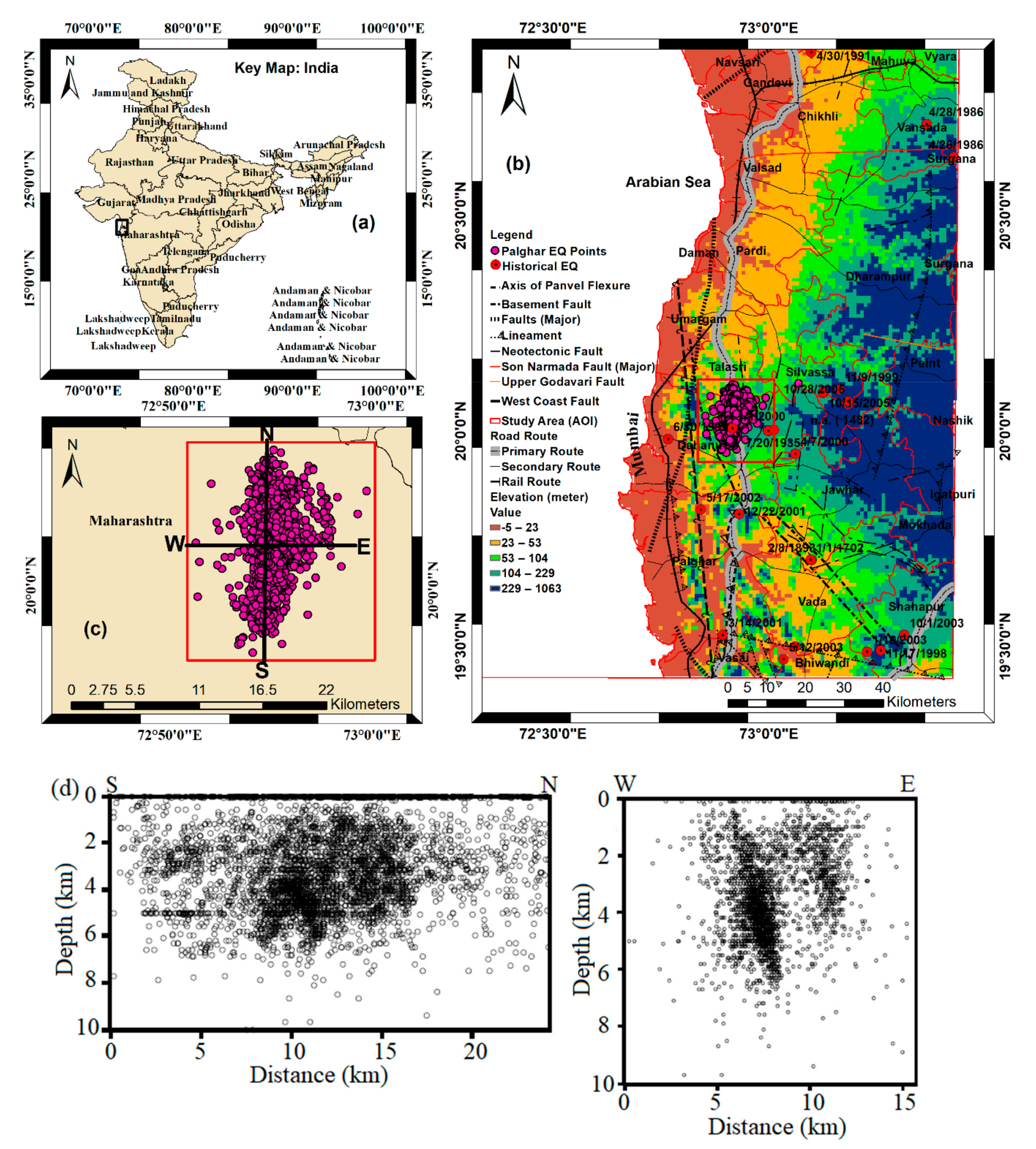
• The earthquakes are clustered in a small area of ~6 × 15 km² to the south of Talasari village encompassing other villages like Dapchari, Modgaon, Haladpada, Pandhartaragaon, Karanjvira, Osarvira, Ambesari, Dhundhalwadi, Shisne, and Deur.
• The majority of the earthquakes (~94%) are found to be located in a shallow depth range between 4.0 to 6.0 km.
• Earthquake swarm activities in the study area show NE–SW and NNE–SSW orientations which is consistent with orientations of lineaments as clearly define the surface strain with ongoing seismicity.
• The results further suggest that earthquake swarm activities are interlinked with the sub-surface geological lineaments with their major orientation changing after 2000, along with the post-monsoon rainfall activities.
• The beginning of swarm activities in the local region may have affected the surrounding region, thus we observed pronounced changes in LD.
• Monthly average soil moisture content (0~10 cm depth) increased which was confirmed also through satellite-derived SMI results. The activity appears to be related to the increased pore pressure in the sub-surface and subsequent crustal adjustments.
• The results of the present study confirm that earthquake swarms might have a relation with the changes in tectonic lineament that could have been triggered combined by crustal motion and monsoon rainfall in the surrounding epicentral region of the 1856 historical earthquake.

References

1. Talwani, P. The intersection model for intraplate earthquakes. Seismol. Res. Lett. 1988, 59, 305–310. [Google Scholar] [CrossRef]
2. Talwani, P.; Rajendran, K. Some seismological and geometric features of intraplate earthquakes. Tectonophysics 1991, 186, 19–41. [Google Scholar] [CrossRef]
3. Seeber, L.; Ekstrom, G.; Jain, S.K.; Murthy, C.V.R.; Chandak, N.; Armbruster, J.J. The 1993 Killari earthquake in central India: A new fault in Mesozoic basalt flows? J. Geophys. Res. 1996, 101, 8543–8560. [Google Scholar] [CrossRef]
4. Gupta, H.K.; Khanal, K.N.; Upadhyan, S.K.; Sarkar, D.; Rastogi, B.K.; Duda, S.J. Verification of magnitudes of Himalayan region earthquakes of 1903–1985 from Gottingen Observatory. Tectonophysics 1995, 244, 267–284. [Google Scholar] [CrossRef]
5. Gupta, H.K.; Mohan, I.; Rastogi, B.K.; Rao, M.N.; Ramakrishna Rao, C.V. A quick look at the Latur earthquake of 30 September 1993. Curr. Sci. India 1993, 65, 517–520. [Google Scholar]
6. Gupta, H.K.; Rao, N.P.; Rastogi, B.K.; Sarkar, D. The deadliest intraplate earthquake. Science 2001, 291, 2101–2102. [Google Scholar] [CrossRef] [PubMed]
7. Banerjee, P.; Bürgmann, R.; Nagarajan, B.; Apel, E. Intraplate deformation of the Indian subcontinent. Geophys. Res. Lett. 2008, 35, L18301. [Google Scholar] [CrossRef]
8. Talwani, P. Intraplate Earthquakes; Cambridge University Press: New York, NY, USA, 2014; ISBN 9781139628921. [Google Scholar]
9. Guha, S.K.; Gosavi, P.D.; Varma, M.M.; Agarwal, B.N.P.; Padale, J.G.; Marwadi, S.C. Recent Seismic Disturbances in the Koyna Hydroelectric Project; Report; Central Water and Power Research Station: Maharashtra, India, 1968. [Google Scholar]
10. Gupta, H.K. The present status of reservoir induced seismicity investigations with special emphasis on Koyna earthquakes. Tectonophysics 1985, 118, 257–279. [Google Scholar] [CrossRef]
11. Guha, S.K.; Gosavi, P.D.; Agarwal, B.N.P.; Padale, J.G.; Marwadi, S.C. Case histories of some artificial crustal disturbances. Eng. Geol. 1974, 8, 59–77. [Google Scholar] [CrossRef]
12. Rastogi, B.K.; Chadha, R.K.; Raju, I.P. Seismicity near Bhatsa reservoir, Maharashtra, India. Phys. Earth Planet. Inter. 1986, 44, 177–199. [Google Scholar] [CrossRef]
13. Rastogi, B.K.; Rao, B.R.; Rao, C.V.R. Microearthquake investigations near Sriramsagar reservoir, Andhra Pradesh, India. Phys. Earth. Planet. Inter. 1986, 4, 149. [Google Scholar] [CrossRef]
14. Rastogi, B.K.; Rap, C.V.R.; Chadha, R.K.; Gupta, H.K. Precursory phenomena in the micro earthquake sequence near the Osmansagar reservoir, Hyderabad, India. Tectonophysics 1987, 138, 17–24. [Google Scholar] [CrossRef]
15. Costain, J.K.; Bollinger, G.A.; Speer, J.A. Hydroseismicity: A hypothesis for the role of water in the generation of intraplate seismicity. Seismol. Res. Lett. 1987, 58, 41–64. [Google Scholar] [CrossRef]
16. Rastogi, B.K.; Sarma, C.S.P.; Chadha, R.K.; Kumar, N. Current seismicity at the Koyna reservoir, Maharashtra, India (1983–84). Gerlands Beitr. Geophys. Leipzig 1990, 99, 229–237. [Google Scholar]
17. Gupta, H.K. Reservoir induced Earthquakes, Development in Geotechnical Engineering 64; Elsevier: Amsterdam, The Netherlands, 1992; p. 320. [Google Scholar]
18. Gupta, H.K. A review of recent studies of triggered earthquakes by artificial water reservoirs with special emphasis on earthquakes in Koyna, India. Earth Sci. Rev. 2002, 58, 279–310. [Google Scholar] [CrossRef]
19. Gupta, H.K.; Rastogi, B.K.; Mohan, I.; Ramakrishna Rao, C.V.; Mishra, D.C.; Rao, G.V.; Rao, R.U.M.; Rao, M.N.; Chetty, T.R.K.; Sarkar, D.; et al. Investigations of Latur Earthquake of September 30, 1993. Geol. Surv. India Spec. Publ. 1995, 27, 17–40. [Google Scholar]
20. Chadha, R.K.; Pandey, A.; Kumpel, H.J. Search for earthquake precursors in well water levels in a localized seismically active area of reservoir triggered earthquakes in India. Geophys. Res. Lett. 2003, 30, 1416. [Google Scholar] [CrossRef]
21. Chadha, R.K.; Singh, C.; Shekar, M. Transient Changes in Well-Water Level in Bore Wells in Western India Due to the 2004 Mw 9.3 Sumatra Earthquake. Bull. Seismol. Soc. Am. 2008, 98, 2553–2558. [Google Scholar] [CrossRef]
22. Yadav, A.; Gahalaut, K.; Purnachandra Rao, N. Role of reservoirs in sustained seismicity of Koyna-Warna region—A statistical analysis. J. Seismol. 2018, 22, 909–920. [Google Scholar] [CrossRef]
23. Officers of the Geological Survey of India. A Geological Report on the Koyna Earthquake of 11th December, 1967, Satara District, Maharashtra State. Unpublished Report (GSI). 1968, p. 242. Available online: https://pdfslide.net/documents/seismotectonics-of-the-koyna-warna-area-seismotectonics-of-the-koyna-warna.html (accessed on 3 November 2021).
24. Singh, D.D.; Rastogi, B.K.; Gupta, H.K. Surface wave radiation pattern and source parameters of the Koyna earthquake of Dec. 10, 1967. Bull. Seismol. Soc. Am. 1975, 65, 711–731. [Google Scholar]
25. Talwani, P.; Kumarswamy, S.V.; Sawalwede, C.B. The Re-Evaluation of Seismicity Data in the Koyna-Warna Area; Report of Univ. of South Carolina; University of South Carolina: Columbia, SC, USA, 1996. [Google Scholar]
26. Talwani, P. Seismotectonics of the Koyna-Warna area, India. Pure Appl. Geophy. 1997, 150, 511–550. [Google Scholar] [CrossRef] [Green Version]
27. Rai, S.S.; Singh, S.K.; Sarma, P.V.S.S.R.; Srinagesh, D.; Reddy, K.N.S.; Prakasam, K.S.; Satyanarayana, Y. What triggers Koyna region earthquakes? Preliminary results from seismic tomography digital array. Proc. Indian Acad. Sci. Earth Planet Sci. 1999, 108, 1–14. [Google Scholar]
28. Pandey, A.P.; Chadha, R.K. Surface loading and triggered earthquakes in the Koyna–Warna region, western India. Phys. Earth Planet. Inter. 2003, 139, 207–223. [Google Scholar] [CrossRef]
29. Gahalaut, V.K.; Kalpna Singh, S.K. Fault interaction and earthquake triggering in the Koyna Warna region, India. Geophys. Res. Lett. 2004, 31, L11614. [Google Scholar] [CrossRef]
30. Pandey, O.P. Shallowing of Mafic Crust and Seismic Instability in the High Velocity Indian Shield. J. Geol. Soc. India 2009, 74, 615–624. [Google Scholar] [CrossRef]
31. Rastogi, B.K.; Santosh, K.; Aggrawal, S.K. Seismicity of Gujarat. Nat. Haz. 2012, 65, 1027–1044. [Google Scholar] [CrossRef]
32. Seeber, L.K. The earthquake that shook the world. New Sci. 1994, 142, 25–29. [Google Scholar]
33. Singh, R.P.; Singh, U.K. Evidence of fluid in the lower crust of Deccan trap region and its possible role in the observed seismicity. Himal. Geol. 1996, 17, 105–111. [Google Scholar]
34. Gupta, H.K.; Rastogi, B.K.; Mohan, I.; Rao, C.V.R.K.; Sarma, S.V.S.; Rao, R.U.M. An investigation into the Latur earthquake of September 29, 1993, in southern India. Tectonophysics 1998, 287, 299–318. [Google Scholar] [CrossRef]
35. Gupta, H.K.; Srinivasan, R.; Rao, R.U.M.; Rao, G.V.; Reddy, G.K.; Roy, S.; Jafri, S.H.; Dayal, A.M.; Zachariah, J.; Parthasarathy, G. Borehole investigations in the surface rupture zone of the 1993 Latur SCR earthquake, Maharashtra, India: Overview of results. In Memoirs-Geological Society of India; Geological Society of India: Bengaluru, India, 2003; pp. 1–22. [Google Scholar]
36. Reddy, C.D.; Sunil, P.S. Post-seismic crustal deformation and strain rate in Bhuj region, western India, after the 2001 January 26 earthquake. Geophys. J. Int. 2008, 172, 593–606. [Google Scholar] [CrossRef] [Green Version]
37. Gupta, S.; Mohanty, W.K.; Prakash, R.; Shukla, A.K. Crustal Heterogeneity and Seismotectonics of the National Capital Region, Delhi, India. Pure Appl. Geophys. 2013, 170, 607–616. [Google Scholar] [CrossRef]
38. Parthasarathy, G.; Pandey, O.P.; Sreedhar, B.; Sharma, M.; Tripathi, P.; Vedanti, N. First observation of microspherule from the infratrappean Gondwana sediments below Killari region of Decan LIP, Maharashtra (India) and possible implications. Geosci. Front. 2019, 10, 2281–2285. [Google Scholar] [CrossRef]
39. Kannaujiya, S.; Gautam, P.K.; Champati ray, P.K.; Chauhan, P.; Roy, P.N.S.; Pal, S.K.; Taloor, A.K. Contribution of seasonal hydrological loading in the variation of seismicity and geodetic deformation in Garhwal region of Northwest Himalaya. Quatern. Int. 2020, 575–576, 62–71. [Google Scholar] [CrossRef]
40. Kolvankar, V.G. Earthquake Sequence of 1991 form Valsad Region, Gujarat; Technical Report, BARC/2001/E/006; BARC: Mumbai, India, 2001. [Google Scholar]
41. Srivastava, H.N.; Bhattacharya, S.N.; Rao, D.T.; Srivastava, S. Strange attractor in earthquake swarms near Valsad (Gujarat), India. Mausam 2007, 58, 543–550. [Google Scholar] [CrossRef]
42. Singh, A.P.; Mishra, O.P. Seismological evidence for monsoon induced micro to moderate earthquake sequence beneath the 2011 Talala, Saurashtra earthquake, Gujarat, India. Tectonophysics 2015, 661, 38–48. [Google Scholar] [CrossRef]
43. Sateesh, A.; Mahesh, P.; Singh, A.P.; Kumar, S.; Chopra, S.; Kumar, M.R. Are earthquake swarms in South Gujarat, northwestern Deccan Volcanic Province of India monsoon induced? Environ. Earth Sci. 2019, 78, 381. [Google Scholar] [CrossRef]
44. Mahesh, P.; Sateesh, A.; Kamra, C.; Kumar, S.; Chopra, S.; Kumar, M.R. Earthquake swarms in Palghar district, Maharasthtra, Deccan Volcanic Province. Curr. Sci. 2020, 118, 701–704. [Google Scholar]
45. Sharma, V.; Wadhawan, M.; Rana, N.; Sreejith, K.M.; Agrawal, R.; Kamra, C.; Hosalikar, K.S.; Narkhede, K.V.; Suresh, G.; Gahalaut, V.K. A long duration non-volcanic earthquake sequence in the stable continental region of India: The Palghar swarm. Tectonophysics 2020, 779, 228376. [Google Scholar] [CrossRef]
46. Srinagesh, D.; Singh, D.K.; Vikas, G.; Naresh, B.; Roy, S.; Murthy, Y.V.V.B.S.N.; Raju, P.S.; Suresh, G.; Mandal, P.; Sharma, A.N.S.; et al. An appraisal of recent earthquake activity in Palghar region, Maharashtra, India. Curr. Sci. 2020, 118, 1592–1598. [Google Scholar] [CrossRef]
47. Hainzl, S.; Aggarawal, S.K.; Khan, P.K.; Rastogi, B.K. Monsoon induced earthquake activity in Talala, Gujarat, India. Geophys. J. Int. 2015, 200, 627–637. [Google Scholar] [CrossRef] [Green Version]
48. Srivastava, S.; Rao, D.T. Present status of seismicity of Gujarat. Vayu Mand. 1997, 27, 32–39. [Google Scholar]
49. Singh, A.P.; Roy, G.I.; Kumar, S.; Kayal, J.R. Seismic source characteristics in Kachchh and Saurashtra regions of western India: B-value and fractal dimension mapping of aftershock sequences. Nat. Haz. 2013, 77, 33–49. [Google Scholar] [CrossRef]
50. Mahesh, P.; Gupta, S. The role of crystallized magma and crustal fluids in intraplate seismic activity in Talala region (Saurashtra), Western India: An insight from local earthquake tomography. Tectonophysics 2016, 690, 131–141. [Google Scholar] [CrossRef]
51. Bhattacharya, S.N.; Karanth, K.V.; Dattatrayam, R.S.; Sohoni, P.S. Earthquake sequence in and around Bhavnagar, Saurashtra, western India during August–December 2000 and associated tectonic features. Curr. Sci. 2004, 86, 1165–1170. [Google Scholar]
52. Jayaraman, K.S. Monsoon behind Low Magnitude Earthquakes in India’s West Coast. Nature India. 3 March 2020. Available online: https://www.nature.com/articles/nindia.2020.39 (accessed on 5 May 2021).
53. Singh, A.P.; Kumar, M.R.; Kumar, S.; Sateesh, A.; Mahesh, P.; Shukla, A.; Talukdar, R. Seismicity and subterranean sounds in the northwest Deccan volcanic province of India. Bull. Seismol. Soc. Am. 2017, 107, 1129–1135. [Google Scholar] [CrossRef]
54. BIS. Criteria for Earthquake Resistant Design of Structures-IS 1893 (Part 1): 2002; General provision and buildings (fifth revision); Bureau of Indian Standards (BIS): New Delhi, India, 2002; p. 39. [Google Scholar]
55. Sibson, R.H. Earthquakes and Lineament Infrastructure. Philos. Trans., Math. Phys. Eng. Sci. 1986, 317, 63–79. [Google Scholar]
56. Joshi, A.; Patel, R.C. Modelling of active lineaments for predicting a possible earthquake scenario around Dehradun, Garhwal Himalaya, India. Tectonophysics. 1997, 283, 289–310. [Google Scholar] [CrossRef]
57. Murthy, Y.S. On the correlation of seismicity with geophysical lineaments over the Indian subcontinent. Curr. Sci. 2002, 83, 760–766. [Google Scholar]
58. Singh, V.P.; Singh, R.P. Changes in stress pattern around epicentral region of Bhuj earthquake of 26 January 2001. Geophys. Res. Lett. 2005, 32, L2430923. [Google Scholar] [CrossRef]
59. Verraswamy, K.; Raval, U. Seismogenic significance of lineaments of the Indian subcontinent. Curr. Sci. 2007, 92, 420–421. [Google Scholar]
60. Bondur, V.G.; Zverev, A.T.; Gaponova, E.V.; Zima, A.L. Space Methods of Studying the Precursor Cycle Dynamics of the Lineament System before the Preparation of Earthquakes. Izv. Atmos. Ocean. Phys. 2019, 55, 1266–1282. [Google Scholar] [CrossRef]
61. Bondur, V.G.; Zverev, A.T.; Gaponova, E.V. Precursor Variability of Lineament Systems detected Using Satellite Images during Strong Earthquakes. Izv. Atmos. Ocean. Phys. 2019, 55, 1283–1291. [Google Scholar] [CrossRef]
62. Cronin, V.S.; Millard, M.; Seidman, L.; Bayliss, B. The Seismo-Lineament Analysis Method (SLAM): A Reconnaissance Tool to Help Find Seismogenic Faults. Environ. Eng. Geosci. 2008, 14, 199–219. [Google Scholar] [CrossRef]
63. Marple, R.T.; Hurd, J.D. Interpretation of lineaments and faults near Summerville, South Carolina, USA, using LiDAR data: Implications for the cause of the 1886 Charleston, South Carolina, earthquake. Atl. Geol. 2020, 56, 73–95. [Google Scholar] [CrossRef]
64. NASA. Giovanni Portal. Meteorological and Geophysical Data Download. Available online: https://giovanni.gsfc.nasa.gov/giovanni/ (accessed on 3 November 2020).
65. Road and Rail Network Distribution. Geofabrik, OpenStreet Map Data. Available online: http://download.geofabrik.de/asia.html (accessed on 10 June 2020).
66. U.S. Geological Survey. Geological Map of South Asia, Data Catalog. 1999. Available online: https://certmapper.cr.usgs.gov/data/we/ofr97470c/spatial/shape/geo8ag.zip (accessed on 5 February 2021).
67. Bansal, B.K.; Gupta, S. A Glance through the Seismicity of Peninsular India. J. Geol. Soc. India 1998, 52, 67–80. [Google Scholar]
68. Mohan, G.; Surve, G.; Tiwari, P.K. Seismic evidences of faulting beneath the Panvel flexure. Curr. Sci. 2007, 93, 991–996. [Google Scholar]
69. Kailasam, L.N.; Murthy, B.G.K.; Chayanulu, A.Y.S.R. Regional gravity studies of the Deccan Trap areas of peninsular India. Curr. Sci. 1972, 41, 403–407. [Google Scholar]
70. Kailasam, L.N.; Reddy, A.G.B.; Jogarao, M.V.; Sathyamurthy, K.; Murty, B.J.K. Deep electrical resistivity sounding in the Deccan Trap region. Curr. Sci. 1976, 45, 9–13. [Google Scholar]
71. Kaila, K.L.; Chowdhury, K.R.; Reddy, P.R.; Krishna, V.G.; Narain, H.; Subbotin, S.I.; Sollogub, V.B.; Chekunov, A.V.; Kharetchko, G.E.; Lazarenko, M.A.; et al. Crustal structure along Kavali-Udipi profile in the Indian peninsular shield from deep seismic sounding. J. Geol. Soc. India 1979, 20, 307–333. [Google Scholar]
72. Kaila, K.L.; Reddy, P.R.; Dixit, M.M.; Lazarenko, M.A. Deep crustal structure at Koyna, Maharashtra, indicated by deep seismic sounding. J. Geol. Soc. India 1981, 22, 1–16. [Google Scholar]
73. Gokaran, S.G.; Rao, C.K.; Singh, B.P.; Nayak, P.N. Magnetotelluric studies across the Kurduwadi gravity feature. Phys. Earth Planet. Inter. 1992, 72, 58–67. [Google Scholar] [CrossRef]
74. Patro, P.K.; Sarma, S.V.S. Lithospheric electrical imaging of the Deccan trap covered region of western India. J. Geophys. Res. Soild Earth 2009, 114, B01102. [Google Scholar] [CrossRef]
75. Pavankumar, G.; Manglik, A. Complex tectonic setting and deep crustal seismicity of the Sikkim Himalaya: An electrical resistivity perspective. Phys. Chem. Earth 2021, 124, 103077. [Google Scholar] [CrossRef]
76. Roy, A.B. Seismicity in the Peninsular Indian Shield: Some geological considerations. Curr. Sci. 2006, 91, 456–463. [Google Scholar]
77. USGS. Earth Explorer Archive. Landsat Imageries Download. Available online: https://earthexplorer.usgs.gov (accessed on 3 November 2020).
78. Singh, R.P.; Bhoi, S.; Sahoo, A.K.; Raj, U.; Ravindranath, S. Surface manifestations after the Gujarat earthquake. Curr. Sci. 2001, 81, 164–166. [Google Scholar]
79. Nath, B.; Niu, Z.; Acharjee, S. Pre-earthquake anomaly detection and assessment through lineament changes observation using multi-temporal Landsat 8-OLI imageries: Case of Gorkha and Imphal. In Multi-Purposeful Application of Geospatial Data; Rustamav, R.B., Hasanova, S., Zeynalova, M.H., Eds.; IntechOpen Ltd.: London, UK, 2018; pp. 149–171. [Google Scholar]
80. Kocal, A.; Duzgun, H.S.; Karpuz, C. Discontinuity Mapping with Automatic Lineament Extraction from High Resolution Satellite Imagery. ISPRS Proceedings-XXXV. 2004. Available online: http://www.isprs.org/proceedings/XXXV/congress/comm7/papers/205.pdf (accessed on 10 February 2021).
81. Nath, B.; Niu, Z.; Singh, R.P. Land Use and Land Cover Changes, and Environment and Risk Evaluation of Dujiangyan City (SW China) Using Remote Sensing and GIS Techniques. Sustainability 2018, 10, 4631. [Google Scholar] [CrossRef] [Green Version]
82. Nath, B.; Niu, Z.; Mitra, A.K. Observation of short-term variations in the clay minerals ratio after the 2015 Chile great earthquake (8.3 Mw) using Landsat 8 OLI data. J. Earth Syst. Sci. 2019, 128, 117. [Google Scholar] [CrossRef] [Green Version]
83. Nath, B.; Wang, Z.; Ge, Y.; Islam, K.; Singh, R.P.; Niu, Z. Land Use and Land Cover Change Modeling and Future Potential Landscape Risk Assessment Using Markov-CA Model and Analytical Hierarchy Process. ISPRS Int. J. Geo-Inf. 2020, 9, 134. [Google Scholar] [CrossRef] [Green Version]
84. Singh, R.P.; Sahoo, A.K.; Bhoi, S.; Kumar, M.G.; Bhuiyan, C. Ground deformation of the Gujarat earthquake of 26 January 2001. Geol. Soc. India 2001, 58, 209–214. [Google Scholar]
85. Dupigny-Giroux, L.; Lewis, J.E. A moisture index for surface characterization over a semiarid area. Photogramm. Eng. Remote Sens. 1999, 65, 937–945. [Google Scholar]
86. Huffman, G.J.; Stocker, E.F.; Bolvin, D.T.; Nelkin, E.J.; Jackson, T. GPM IMERG Final Precipitation L3 1 Month 0.1-Degree x 0.1-Degree V06; Goddard Earth Sciences Data, and Information Services Center (GES DISC): Greenbelt, MD, USA, 2019. [Google Scholar]
87. Gutenberg, R.; Richter, C.F. Frequency of earthquakes in California. Bull. Seismol. Soc. Am. 1944, 34, 185–188. [Google Scholar] [CrossRef]
88. Gutenberg, B.; Richter, C.F. Seismicity of the Earth and Associated Phenomena, 2nd ed.; Princeton University Press: Princeton, NJ, USA, 1954. [Google Scholar]
89. Wiemer, S.; Wyss, M. Minimum magnitude of completeness in earthquake catalogs: Example from Alaska, the western US and Japan. Bull. Seismol. Soc. Am. 2000, 90, 859–869. [Google Scholar] [CrossRef]
90. Woessner, J.; Wiemer, S. Assessing the quality of earthquake catalogues: Estimating the magnitude of completeness and Its Uncertainty. Bull. Seismol. Soc. Am. 2005, 95, 684–698. [Google Scholar] [CrossRef]
91. Brudzinski, M.R.; Kozlowska, M. Seismicity induced by hydraulic fracturing and wastewater disposal in the Appalachian Basin, USA: A review. Acta Geophys. 2019, 67, 351–364. [Google Scholar] [CrossRef] [Green Version]
92. Villa, V.; Singh, R.P. Hydraulic fracturing operation for oil and gas production and associated earthquake activities across the USA. Environ. Earth Sci. 2020, 79, 271. [Google Scholar] [CrossRef]
93. Ellsworth, W.L. Injection-induced earthquakes. Science 2013, 341, 1225942. [Google Scholar] [CrossRef]
94. Kim, W. Induced seismicity associated with fluid injection into a deep well in Youngstown, Ohio. J. Geophys. Res. Solid Earth 2013, 118, 3506–3518. [Google Scholar] [CrossRef]
95. Westwood, R.F.; Toon, S.M.; Styles, P.; Cassidy, N.J. Horizontal respect distance for hydraulic fracturing in the vicinity of existing faults in deep geological reservoirs: A review and modelling study. Geotech. Geophys. Geo-Energ. Geo-Resour. 2017, 3, 379–391. [Google Scholar] [CrossRef]
96. Wilson, M.P.; Worrall, F.; Davies, R.J.; Almond, S. Fracking: How far from faults? Geomech. Geophys. Geo-Energ. Geo-Resour. 2018, 4, 193–199. [Google Scholar] [CrossRef] [Green Version]
97. Wu, Q.; Chapman, M.; Chen, X. Stress-Drop Variations of Induced Earthquakes in Oklahoma. Bull. Seismol. Soc. Am. 2018, 108, 1107–1123. [Google Scholar] [CrossRef]
98. Pei, S.; Peng, Z.; Chen, X. Locations of Injection-Induced Earthquakes in Oklahoma Controlled by Crustal Structures. Geophys. Res.-Solid Earth 2018, 123, 2332–2344. [Google Scholar] [CrossRef]
99. Richter, G. Stress-based, statistical modeling of the induced seismicity at the Groningen gas field, The Netherlands. Environ. Earth Sci. 2020, 79, 252. [Google Scholar] [CrossRef]
100. Singh, R.P.; Sato, T.; Nyland, E. The geodynamic context of the Latur (India) earthquake of September 30, 1993. Phys. Earth Planet Int. 1995, 91, 245–251. [Google Scholar] [CrossRef]
101. Singh, R.P.; Mehdi, W.; Naeimi, M.; Sahoo, A.; Kumar, R. Analysis of widespread fissures associated with groundwater depletion and extreme rainfall using multi sensor data. IAHS 2011, 343, 28–33. [Google Scholar]
102. He, A.; Zhao, G.; Sun, Z.; Singh, R.P. Co-seismic multilayer water temperature and water level changes associated with Wenchuan and Tohoku-Oki earthquakes in the Chuan no. 03 well China. J. Seism. 2017, 21, 719–734. [Google Scholar] [CrossRef]
103. He, A.; Fan, X.; Zhao, G.; Liu, Y.; Singh, R.P.; Hu, Y. Co-seismic Response of Water Level in the Jingle Well (China) Associated with the Gorkha Nepal (Mw 7.8) earthquake. Tectonophysics 2017, 714, 82–89. [Google Scholar] [CrossRef]
104. Brodsky, E.E.; Roeloffs, E.; Woodcock, D.; Gall, I.; Manga, M. A mechanism for sustained groundwater pressure changes induced by distant earthquakes. J. Geophys. Res. 2003, 108, 2390. [Google Scholar] [CrossRef] [Green Version]
105. Paul, J.; Bürgmann, R.; Gaur, V.K.; Bilham, R.; Larson, K.M.; Ananda, M.B.; Jade, S.; Mukal, M.; Anupama, T.S.; Satyal, G.; et al. The motion and active deformation of India. Geophys. Res. Lett. 2001, 28, 647–650. [Google Scholar] [CrossRef] [Green Version]
106. Farquharson, J.; Amelung, F. Extreme rainfall triggered the 2018 rift eruption at Kīlauea Volcano. Nature 2020, 580, 491–495. [Google Scholar] [CrossRef]
107. Heinicke, J.; Fischer, T.; Gaupp, R.; Gotze, J.; Koch, U.; Konietzky, H.; Stanek, K.-P. Hydrothermal alteration as a trigger mechanism for earthquake swarms: The Vogtland/NW Bohemia region as a case study. Geophys. J. Int. 2009, 178, 1–13. [Google Scholar] [CrossRef] [Green Version]
108. Srivastava, H.N.; Dube, R.K. Comparison of precursory and non-precursory swarm activity in peninsular India. Tectonophysics 1996, 265, 327–339. [Google Scholar] [CrossRef]
109. Naidu, G.D.; Khupat, S.; Awasthi, D.K. Deciphering the seismicity pattern from MEQ study at Indra Sagar reservoir area, Madhya Pradesh, India. J. Ind. Geophys. Union 2015, 19, 55–61. [Google Scholar]
110. Rao, D.T.; Jambusaria, B.B.; Srivastava, S.; Srivastava, N.P.; Hamid, A.; Desai, B.N.; Srivastava, H.N. Earthquake swarm activity in south Gujarat. Mausam 1991, 42, 89–98. [Google Scholar] [CrossRef]
111. Hainzl, S.; Kraft, T.; Wassermann, J.; Igel, H.; Schmedes, E. Evidence for rainfall-triggered earthquake activity. Geophys. Res. Lett. 2006, 33, L19303. [Google Scholar] [CrossRef] [Green Version]
112. Pimprikar, S.D.; Mylappally, D. Earthquake swarm activity around village Bamhori, Seoni District, Madhya Pradesh: A preliminary study. J. Geol. Soc. India 2003, 62, 498–502. [Google Scholar]
113. Horálek, J.; Fischer, T.; Einarsson, P.; Jakobsdóttir, S.S. Earthquake Swarms. In Encyclopedia of Earthquake Engineering; Springer: Berlin/Heidelberg, Germany, 2014; pp. 871–885. [Google Scholar] [CrossRef]
114. Horálek, J.; Fischer, T.; Boušková, A.; Michálek, J.; Hrubcová, P. The West Bohemian 2008-earthquake swarm: When, where what size and data. Stud. Geophys. Geod. 2009, 53, 351–358. [Google Scholar] [CrossRef]
115. Gahalaut, K.; Gahalaut, V.K. Stress triggering of normal aftershocks due to strike slip earthquakes in compressive regime. J. Asian Earth Sci. 2008, 33, 379–382. [Google Scholar] [CrossRef]
116. He, A.; Singh, R.P. Groundwater level response to the Wenchuan earthquake of May 2008. Geomat. Nat. Haz. Risk. 2019, 10, 336–352. [Google Scholar] [CrossRef] [Green Version]
117. Gahalaut, K.; Hassoup, A. Role of fluids in the earthquake occurrence around Aswan reservoir. Egypt. J. Geophys. Res. 2012, 117, B02303. [Google Scholar] [CrossRef] [Green Version]
118. Bhattacharya, S.N.; Dattatrayam, R.S. Some characteristics of recent earthquake sequences in Peninsular India. Gond. Geol. Magz. Spl. 2003, 5, 67–85. [Google Scholar]
Figure 1. (a) Location map of the study area; (b) shows entire study area (broad regions) with digital elevation model (DEM) map and with recently observed earthquake swarms shown with solid magenta color (small area with red bounding box) and historical earthquakes (red color dot) data; (c) earthquakes swarms in zoom view with two transect lines North-South (N-S) and East-West (E-W) and (d) shows depth distribution of earthquakes along N-S (left panel) and E-W (right panel).
Remotesensing 14 00135 g001
Figure 2. 3D Terrain structure of the Indian shield, general geology and other geographical distribution of the study area; (a) 3D view of the terrain of the Indian shield areas (3D image using Land Viewer 2020); and red bounding box on this image shows broad regions of the study area applicable for Figure 2b,c. (b) General geology (masking from Geologic map of South Asia shapefile; https://certmapper.cr.usgs.gov/data/ accessed on 3 November 2020) [66] with other geographical information such as road and rail network distribution (masking from Geofabrik, OpenStreet Map data; http://download.geofabrik.de/asia.html (accessed on 3 November 2021)) [65] with recent Palghar earthquake swarm epicenters (3.5 ≤ ML) and historical earthquakes (5.7 ≤ ML) distribution since 1702–2005 (based on all available earthquake catalog, taken from 1200 AD to 2005) [34,67,68] where only 24 points (details of earthquake are given in Appendix A Table A1) are recorded within our AOI (red rectangle box); (c) Regional faults distribution in the western parts of India along with location of the observed earthquake swarms (distribution of earthquake epicenters during January and December 2020) and 10 km buffer zone created around highway NH-8 because recent earthquake swarms are clustered within buffer zone and along with historical earthquake points displaying over geology and regional faults.
Remotesensing 14 00135 g002
Figure 3. Frequency magnitude distribution with respect to ML. The straight line is the best fit by Gutenberg and Richter (1941). The threshold magnitude, MC (triangle), and overall b-value with standard deviation are also displayed.
Remotesensing 14 00135 g003
Figure 4. Lineaments and lineaments density (LD) distribution of the study areas (broad regions) during 2000–2020; (a) lineaments of the year 2000 is associated with the past earthquakes; (b) lineament density generated based on lineaments of the year 2000; (c) lineaments retrieved during the year 2015 with past earthquakes; (d) lineament density generated based on lineaments of 2015; (e) lineaments extracted in the year 2018 earthquakes; (f) lineament density generated based on lineaments of 2018; (g) lineaments of 2019 with ongoing earthquake swarms and past earthquakes; (h) lineament density generated based on lineaments of 2019; (i) lineaments of 2020 with available earthquake swarm points and past earthquakes; (j) lineament density generated based on extracted lineaments of 2020 to represent the present scenario of stress changes in the study area.
Remotesensing 14 00135 g004aRemotesensing 14 00135 g004bRemotesensing 14 00135 g004c
Figure 5. LD distribution of the swarm regions and its comparison with broad regions during 2000–2020; (a) LD distribution of 2000 of the swarm regions; (b) LD distribution of 2015 of the swarm regions; (c) LD distribution of 2018 of the swarm regions; (d) LD distribution of 2019 of the swarm regions; (e) LD distribution of 2020 of the swarm regions, and (f) LDmax value comparison in swarm regions with broad regions to know stress development pattern through the similar time interval. The error bar in both swarm and broad regions indicates the standard error of the mean data values.
Remotesensing 14 00135 g005
Figure 6. Spatial variation of Soil Moisture over the land and ocean part using the Soil Moisture Index (SMI) from 2000–2020; (a) SMI status of 2000; (b) SMI status of 2015; (c) SMI status of 2018; (d) SMI status of 2019; (e) SMI status of 2020. In each image, the inside red bounding box represents swarm regions.
Remotesensing 14 00135 g006aRemotesensing 14 00135 g006bRemotesensing 14 00135 g006c
Figure 7. Earthquake 2D depth model and 3D view of earthquake swarms data with spatial variations of earthquakes depth and transects profiles at different sections (horizontal, vertical, and aligned to major fault directions); (a) earthquake depth map with the frequency of earthquakes according to depth variations; (b) Horizontal transects over grayscale depth image constructed from west to east direction for profile construction; (c) Vertical transects constructed over grayscale depth image from North-South direction as lower bottom panel represents VT profiles 1–4, and top-bottom panel represents HT profiles of 1–4, respectively; (d) 3D mesh view of earthquakes displaying according to the varied depth of earthquake occurrences in the study area: Dark red open circles represent depth <5.0 km whilst blue colors show depth >5.0 km.
Remotesensing 14 00135 g007aRemotesensing 14 00135 g007b
Figure 8. Examining earthquakes association with the meteorological and geophysical parameters; (a) monthly total earthquakes with monthly rainfall distribution; (b) associations examining monthly earthquakes with soil moisture content at 0–10 cm underground, and (c) associations examining with monthly earthquakes total with surface skin temperature.
Remotesensing 14 00135 g008
Publisher’s Note: MDPI stays neutral with regard to jurisdictional claims in published maps and institutional affiliations.