Comparison of Marine Gravity Measurements from Shipborne and Satellite Altimetry in the Arctic Ocean

Abstract

To understand the influence of sea ice on shipborne gravity measurements and the accuracy of the satellite-altimetry-derived gravity field in the Arctic Ocean, we compared shipborne gravity measurements with those obtained from satellite altimetric gravity measurements. The influence of sea ice on the shipborne gravity measurements was mainly concentrated in the 0–6 km wavelength range, and the standard deviation of the noise amplitudes was 2.62 mGal. Compared to ice-free regions, the accuracies in the region with floating ice were reduced by 13% for DTU21 and 6% for SV31. Due to the influence of sea ice, satellite altimetric gravity data lose significant information in the 9–12 km wavelength range. The coherence curve of the shipborne gravity with bathymetry was nearly the same as that of the satellite altimetric gravity. The satellite data contain nearly all of the significant information that is present in the shipborne data. The differences between the shipborne and satellite gravity data are small and can be used to study the crustal structure of the Arctic.

1. Introduction

Marine gravity data can provide important constraints on the density structure of the lithosphere [1,2,3,4]. With the development and application of satellite technology, satellite altimetry data have become the important data source for marine gravity fields. In recent years, a number of new satellite altimetry missions, such as Jason-2, Cryosat-2, Altika and Sentinel-3A, have been launched [5,6,7], which significantly increases the amount of altimetry data available for marine gravity field determinations. This greatly improves the resolution of global gravity fields and causes the data quality in some regions to be comparable with that of shipborne gravity observations [8].

The harsh environment and cover of sea ice in the Arctic Ocean seriously hinder the collection of geophysical and geological data. The satellite altimetric gravity field model has become the main tool to study the lithospheric structure of the Arctic Ocean. Therefore, a quantitative analysis of the accuracy of the current Arctic gravity model is important for the study of its geological structure. In ice-covered regions, complex radar echoes confuse the data processor and corrupt the standard altimetric data products [9]. Although altimetric gravity data can be derived by reprocessing the data from the ice-covered regions [10], the data quality is reduced compared to that of ice-free regions [9]. In addition, the shipborne gravity data contain noise due to the collision between the ship and the sea ice [11]. Currently, the influence of sea ice on gravity measurements and the accuracy of the current gravity model in the Arctic Ocean are still unclear due to the scarcity of shipborne gravity data.

Since 1999, China has carried out 11 Arctic research expeditions, which have obtained large amounts of shipborne gravity data and multibeam bathymetry data. This provides us with a good opportunity to analyze the influence of sea ice on gravity measurements and assess the accuracy of the current gravity model in the Arctic Ocean. By using the shipborne gravity and multibeam bathymetry data that were collected by five Arctic research expeditions, the satellite-derived gravity model, and the sea ice thickness and concentration data, we analyzed the spectra of the shipborne gravity data from the ice-covered regions, the differences and coherences between the shipborne and satellite altimetric gravity data, as well as the coherence between gravity and bathymetry. This not only provides reliable data analysis results for scholars to study polar regions by using gravity data, but also provides a basis for improving the processing method for gravity data in polar regions.

2. Data

Here, we selected the shipborne gravity data of five Arctic research expeditions, including the fifth Arctic research expedition in 2012, the sixth Arctic research expedition in 2014, the seventh Arctic research expedition in 2016, the ninth Arctic research expedition in 2018, and the eleventh Arctic research expedition in 2020. We refer to these data as Arctic-12, Arctic-14, Arctic-16, Arctic-18, and Arctic-20, respectively. The Chinese icebreaker research vessel employed was “Xuelong”, which has the ability to break 1.2 m of ice and 0.2 m of snow while operating at a speed of 1.5 knots. We selected gravity survey lines with speed changes of no more than 1 knot, course changes of no more than 10°, and measurement times of more than 60 min as the effective data. We selected 119 gravity survey lines with a total of 2,833,023 observed points (

Table 1. Information on gravity survey for each cruise of Arctic research expeditions.

	Survey Lines	Number of Observations	Length (km)	Minimum (mGal)	Maximum (mGal)	Mean (mGal)	Standard Deviation (mGal)
Arctic−12	29	906,789	11,062	−49.6	129.3	2.9	22.3
Arctic−14	20	717,961	2124	−72.4	59.3	−6.3	19.1
Arctic−16	15	375,841	2239	−78.8	39.9	−10.9	16.6
Arctic−18	15	180,014	1088	−58.6	69.8	5.6	36.8
Arctic−20	40	652,418	4486	−42.9	44.1	4.0	17.8

, Figure 1). We processed the original gravity data and corrected for various errors, including time constant corrections, normal field corrections, Eotvos corrections, zero drift corrections, and free-air corrections, to obtain the free-air gravity anomalies (FAA, Table 1). Figure 2 shows the crossover errors of the five Arctic research expeditions. In the ice-free regions, the crossover error was mostly less than 2 mGal. The average crossover errors of Arctic-12, Arctic-14, Arctic-18, and Arctic-20 are 0.48, 0.99, 0.33, and 0.4 mGal, respectively. In ice-covered regions, the average crossover error is 2.7 mGal due to the influence of sea ice. The Arctic-18 and Arctic-20 data featured the densest survey lines (Figure 1), which were generally closer than 4 km. In addition, Arctic-18 and Arctic-20 also collected multibeam bathymetry data. Therefore, we used the gravity data and multibeam bathymetry data of Arctic-18 and Arctic-20 for a two-dimensional comparison with the satellite altimetric gravity data.

Here, we used the latest global marine gravity datasets that contain new altimetry data from two polar-orbiting satellites (e.g., Cryosat-2 and SARAL/AltiKa): the DTU21 gravity model at 1′ × 1′ from the Danish Technical University and the satellite-altimetry-derived free-air gravity model at 1′ × 1′ provided by Sandwell et al. [12]—version 31.1—hereafter referred to as “SV31”. DTU21 used the EGM2008 gravity model [13] to fill north of 88° N in order to ensure global coverage. However, the data coverage of SV31 is limited to 80° N/S.

Sea ice thickness and concentration data were provided by the Polar Science Center. These data were derived from the Global Ice Ocean Modelling and Assimilation System (GIOMAS) [14,15,16].

3. Data Comparison and Analysis

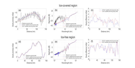
3.1. One-Dimensional Analysis

The satellite altimetric gravity data were sampled along the ship tracks, and the shipborne gravity data were resampled at 1′ intervals to match the satellite-altimetry-derived gravity field.

The gravity survey lines were divided into 55 ice-covered gravity survey lines and 64 ice-free gravity survey lines according to the sea ice thickness and concentration data and some voyage reports (Arctic-14 and Arctic-16). When the ice conditions were extreme, low-frequency gravity data were superimposed with a large number of high-frequency noise (Figure 3). We calculated the power spectra of the shipborne and satellite altimetric gravity data (red lines in Figure 1) that were seriously affected by sea ice at different wavelength ranges by using fast Fourier transforms to investigate the wavelength range of the influence of sea ice on shipborne gravity measurements (Figure 3). Profiles Ice-3 and Ice-4 only featured DTU21 gravity data due to the fact that they were located north of 80°N, which is outside the data range of SV31. As shown in Figure 3, at wavelengths greater than 10 km, the power spectrum curve of the shipborne gravity data was in good overall agreement with those of DTU21 and SV31, which indicates that their waveforms featured good consistency at long wavelengths. When the wavelengths were less than 10 km, the power spectrum curves of the DTU21 and SV31 data dropped rapidly, while the curve of the shipborne gravity data remained unchanged or even rose. This was due to the fact that satellite-altimetry-derived free-air gravity data did not recover a wavelength shorter than 10 km. When the wavelengths are less than 6 km, the power spectrum curves of the shipborne gravity data became significantly uneven, indicating that the gravity data were disturbed by noise. We speculate that this was likely to have resulted from sea ice. The collision between the ship and the sea ice made the speed and direction of the ship change dramatically, resulting in high frequency gravity noise. Therefore, we suggest that the influence of sea ice on shipborne gravity measurements was mainly concentrated in the 0–6 km wavelength range. The shipborne gravity data were filtered by using a Blackman filter in order to eliminate the noise caused by the sea ice. In addition, to better quantify the influence of sea ice on the shipborne gravity measurements, we compared the differences between the unfiltered and filtered shipborne gravity data. The standard deviation of the differences between the unfiltered and filtered shipborne gravity data was 2.62 mGal, which can be regarded as the amplitude of the influence of sea ice on the shipborne gravity measurements.

We calculated the differences between the shipborne and satellite altimetric gravity data over the ice-covered and ice-free regions (Figure 4) in order to analyze the influence of sea ice on satellite altimetric gravity and the accuracy of the new satellite-altimetry-derived gravity fields (DTU21 and SV31) in the Arctic Ocean. In the ice-free regions, the standard deviations of the differences between the shipborne and satellite altimetric gravity data were 3.1 mGal for DTU21 and 3.1 mGal for SV31. In the ice-covered regions, the standard deviations of the differences between the shipborne data and DTU21 data and the SV31 data were 3.5 and 3.3 mGal, respectively. Due to the influence of sea ice, the accuracies of the DTU21 and SV31 data were reduced by 13 and 6%, respectively. Andersen and Knudsen [17] analyzed the accuracy of DTU17 gravity data in the Arctic Ocean by comparing DTU17 with high-quality airborne data flown north of Greenland. The results showed that the standard deviation of the difference between the airborne gravity data and DTU17 was 3.78 mGal. Therefore, the accuracy of DTU21 was improved by 7–13% in the Arctic Ocean. This was primarily due to the recent inclusion of the new Cryosat-2 and SARAL/AltiKa satellite altimeter data.

We also calculated the coherence between shipborne and satellite altimetric gravity. The coherence curve tended to 1, which indicates that the shipborne and satellite altimetric gravity curves featured nearly the same waveforms. Since shorter gravity survey lines contain less wavelength information, we selected lines with lengths greater than 80 km for the coherence analysis. The coherence transition wavelength (CTW) is defined as the wavelength at which the coherence is 0.5 and can be regarded as an approximation of the wavelength at which the transition from a coherent curve to an incoherent curve occurs [18,19]. Figure 5 shows the CTWs of the ice-covered and ice-free gravity data. In the ice-covered regions, the satellite altimetric gravity data were nearly incoherent with the shipborne gravity data below a wavelength of 10 km, and the CTWs of some gravity survey lines were even greater than 17 km. However, in the ice-free regions, the maximum CTW was 11.8 km, and at some points, the coherence between the shipborne and the satellite altimetric gravity reached 5.2 km. The average CTWs of the ice-covered and ice-free gravity data are 12–12.9 and 9.2–9.5 km, respectively, which indicate that the satellite altimetric gravity data lose significant information in the 9–12 km wavelength range due to the influence of sea ice.

3.2. Two-Dimensional Analysis

A two-dimensional comparison of the FAAs that were derived from satellite altimetry with those that were obtained from the shipborne gravity data of Arctic-18 and Arctic-20 was conducted in order to more comprehensively analyze the accuracy and application of satellite altimetric gravity data in the Arctic Ocean. To better quantify the differences between the shipborne and satellite altimetric gravity data, we gridded the shipborne gravity data at 1′ × 1′ intervals and limited the comparison range to the region covered by the shipborne data. The Arctic-18 data were located at Northwind Basin. Figure 6a shows the shipborne free-air gravity anomaly. The survey area covered an area of approximately 5000 km². Figure 6b shows the multibeam bathymetry in the survey area, and the water depths vary from 650 to 2220 m. The eastern and western parts of the survey area feature two obvious areas with high terrain where the water depths are below 1000 m. The water depths in the middle of the survey area exceed 2000 m, except for two linear uplifts with 1500 m water depths in the south. Figure 6c,e show the free-air gravity anomalies (FAA) for the SV31 and DTU21 data, respectively. The overall FAA variation patterns of the shipborne and satellite altimetry looked very similar and agreed well with the topography. Figure 6d,f show the differences between the shipborne gravity data and SV31 and DTU21 data, respectively. The standard deviations of the differences between the shipborne gravity data and satellite altimetric gravity data were 5.0 mGal for SV31 and 5.6 mGal for DTU21.

The Arctic-20 data were located on the Mendeleev Ridge and Chukchi Basin. Figure 7a shows the shipborne FAA. The survey area covered an area of approximately 9360 km². Figure 7b shows the multibeam bathymetry in the survey area. The water depths range from approximately 500 m on the Mendeleev Ridge in the western part of the survey area to approximately 2100 m in the Chukchi Basin. Figure 7c,e show the FAA for SV31 and DTU21, respectively. The shipborne and satellite altimetric gravity data showed good consistency in the western part of the survey area, but there were some differences in the eastern part of the survey area. The FAA map of the shipborne data shows a higher resolution than that of the satellite data. As shown in Figure 7b, there are some uplifts in the transition zone between the Mendeleev Ridge and Chukchi Basin, and the topographic gradient is steep. These short-wavelength features can be seen in the ship’s FAA map. Figure 7d,f show the differences between the shipborne gravity data and SV31 and DTU21, respectively. The standard deviations of the differences between the shipborne gravity data and the satellite altimetric gravity data were 5.2 mGal for SV31 and 3.9 mGal for DTU21.

We compared the bathymetry, shipborne gravity, and satellite altimetric gravity data in the wavenumber domain. In the absence of noise, FAAs are dominated by the attraction of the seafloor/water interface [20]. Therefore, FAA variations should be consistent with the topography. Figure 8 shows the coherences of the bathymetry with the gravity fields from the shipborne and satellite altimetric data. In the Arctic-18 region, the CWT of the shipborne gravity was 18.6 km, versus 19.5 km for the DTU21 and 19.5 km for the SV31 data (Figure 8a). In the Arctic-20 region, the CWT of shipborne gravity was 16.8 km, versus 17.7 km for DTU21 and 17.9 km for SV31 (Figure 8b). The coherence in the Arctic-18 region was obviously lower than that in the Arctic-20 region at long wavelengths, which indicates that the lithosphere of the Arctic-18 region was in a relatively non-isostatic state compared with that of the Arctic-20 region. Overall, the coherence curve of the shipborne gravity was nearly the same as that of satellite altimetric gravity, which indicates that the satellite data contained nearly all of the significant information that was present in the shipborne data.

Gravity anomaly data are mainly used to study crustal thicknesses and density variations, while the noisy and filtered nature of satellite gravity measurements limit their application [20]. To verify the accuracy of the satellite-altimetry-derived gravity field for quantitative regional studies of the Arctic Ocean, we interpreted the FAAs in terms of crustal thickness variations. In the Arctic-18 region, the standard deviation of the amplitudes of the variations in crustal thickness derived from shipborne FAAs was 3330 m, while the standard deviation of the amplitudes of the variations in crustal thickness derived from the differences between shipborne and satellite altimetric FAAs was 450–600 m. In the Arctic-20 region, the standard deviation of the amplitudes of the variations in crustal thickness derived from the shipborne FAAs was 3,700 m, while the standard deviation of the amplitudes of the variations in crustal thickness that were derived from the differences between the shipborne and satellite altimetric FAAs was 350–450 m. The erroneous variations in crustal thickness that were created by the differences between the shipborne and satellite altimetric gravity accounted for only 9–18% of the variations in crustal thickness in our survey area. Therefore, a new satellite-altimetry-derived gravity field can be used to study the regional crustal structure of the Arctic Ocean.

4. Conclusions

The influence of sea ice on the shipborne gravity measurements is mainly concentrated in the 0–6 km wavelength range, according to the power spectrum analysis. The standard deviation of the amplitudes of the influences of sea ice on the shipborne gravity measurements was 2.62 mGal.

In the ice-free regions, the standard deviations of the differences between the shipborne and satellite altimetric gravity data were 3.1 mGal for DTU21 and 3.1 mGal for SV31. Compared with DTU17, the accuracy of DTU21 was improved by 7–13% in the Arctic Ocean. In the ice-covered regions, the standard deviations of the differences between the shipborne and satellite altimetric gravity data were 3.5 mGal for DTU21 and 3.3 mGal for SV31, whose accuracies were reduced by 13 and 6%, respectively, compared with the ice-free regions. The satellite altimetric gravity data lost significant information in the 9–12 km wavelength range due to the influence of sea ice.

The coherence curve of the shipborne gravity with bathymetry was nearly the same as that of the satellite altimetric gravity. The satellite altimetric gravity data contained nearly all of the significant information contained in the shipborne data, and the differences between the shipborne and satellite altimetric gravity data created few erroneous variations in crustal thickness; therefore, a new satellite-altimetry-derived gravity field can be an essential tool for studying the crustal structure of the Arctic Ocean.

References

1. Blackman, D.K.; Forsyth, D.W. Isostatic compensation of tectonic features of the Mid-Atlantic Ridge: 25–27°30′ S. J. Geophys. Res. Solid Earth 1991, 22, 883–892. [Google Scholar] [CrossRef]
2. Kuo, B.Y.; Forsyth, D.W. Gravity anomalies of the ridge-transform system in the South Atlantic between 31 and 34.5° S: Upwelling centers and variations in the crustal thickness. Mar. Geophys. Res. 1988, 96, 11741–11758. [Google Scholar] [CrossRef]
3. Lin, J.; Purdy, G.M.; Schouten, H.; Sempéré, J.C.; Zervas, C. Evidence from gravity data for focused magmatic accretion along the Mid-Atlantic Ridge. Nature 1990, 344, 627–632. [Google Scholar] [CrossRef]
4. Morris, E.; Detrick, R.S. Three-dimensional analysis of gravity anomalies in the MARK area, Mid-Atlantic Ridge 23° N. J. Geophys. Res. Solid Earth 1991, 96, 4355–4366. [Google Scholar] [CrossRef]
5. Kwok, R. Simulated Effects of a Snow Layer on Retrieval of CryoSat-2 Sea Ice Freeboard. Geophys. Res. Lett. 2014, 41, 5014–5020. [Google Scholar] [CrossRef]
6. Hector, H.S.; Pierre, Q.; Fabrice, A. Assessment of SARAL/AltiKa Wave Height Measurements Relative to Buoy, Jason-2, and Cryosat-2 Data. Mar. Geod. 2015, 38, 449–465. [Google Scholar] [CrossRef] [Green Version]
7. Shen, X.; Ke, C.Q.; Xie, H.; Li, M.; Xia, W. A comparison of Arctic sea ice freeboard products from Sentinel-3A and CryoSat-2 data. Int. J. Remote Sens. 2020, 41, 2789–2806. [Google Scholar] [CrossRef]
8. Christensen, A.N.; Andersen, O.B. Comparison of Satellite Altimetric Gravity and Ship-borne Gravity—Offshore Western Australia. In Proceedings of the ASEG-PESA-AIG 2016, Adelaide, Australis, 21–24 August 2016. [Google Scholar] [CrossRef] [Green Version]
9. Andersen, O.B.; Forsberg, R.; Knudsen, P.; Laxon, S.; McAdoo, D. Comparison of Altimetric and Ship borne Marine Gravity over Ice-free and Ice-covered polar Seas. In Geodesy on the Move-Gravity, Geoid, Geodynamics and Antarctica; Forsberg, R., Feissel, M., Dietrich, R., Eds.; Springer: Berlin/Heidelberg, Germany, 1998; Volume 119, pp. 492–497. ISBN 978-3-642-72245-5. [Google Scholar]
10. Laxon, S.W.; McAdoo, D. Arctic Ocean Gravity Field Derived From ERS-1 Satellite Altimetry. Science 1994, 265, 621–624. [Google Scholar] [CrossRef]
11. Urlaub, M.; Schmidt-Aursch, M.C.; Jokat, W.; Kaul, N. Gravity crustal models and heat flow measurements for the Eurasia Basin, Arctic Ocean. Mar. Geophys. Res. 2009, 30, 277–292. [Google Scholar] [CrossRef]
12. Sandwell, D.T.; Müller, R.D.; Smith, W.H.; Garcia, E.; Francis, R. New global marine gravity model from CryoSat-2 and Jason-1 reveals buried tectonic structure. Science 2014, 346, 65–67. [Google Scholar] [CrossRef]
13. Pavlis, N.K.; Holmes, S.A.; Kenyon, S.C.; Factor, J.K. The development and evaluation of the Earth Gravitational Model 2008 (EGM2008). J. Geophys. Res. Solid Earth 2012, 117, B04406. [Google Scholar] [CrossRef] [Green Version]
14. Zhang, J.; Rothrock, D.A. Modeling global sea ice with a thickness and enthalpy distribution model in generalized curvilinear coordinates. Mon. Weather. Rev. 2003, 131, 681–697. [Google Scholar] [CrossRef] [Green Version]
15. Lindsay, R.W.; Zhang, J.; Schweiger, A.; Steele, M.A. Seasonal predictions of ice extent in the Arctic Ocean. J. Geophys. Res. Atmos. 2008, 113, C02023. [Google Scholar] [CrossRef] [Green Version]
16. Schweiger, A.R.; Lindsay, J.; Zhang, J.; Steele, M.A.; Stern, H. Uncertainty in modeled arctic sea ice volume. J. Geophys. Res. 2011, 116, C00D06. [Google Scholar] [CrossRef] [Green Version]
17. Andersen, O.B.; Knudsen, P. The DTU17 Global Marine Gravity Field: First Validation Results. In Fiducial Reference Measurements for Altimetry; Mertikas, S., Pail, R., Eds.; Springer: Berlin/Heidelberg, Germany, 2019; Volume 150, pp. 83–87. ISBN 978-3-030-39437-0. [Google Scholar]
18. Pérez-Gussinyé, M.; Metois, M.; Fernández, M.; Vergés, J.; Fullea, J.; Lowry, A.R. Effective elastic thickness of Africa and its relationship to other proxies for lithospheric structure and surface tectonics. Earth Planet. Sci. Lett. 2009, 287, 152–167. [Google Scholar] [CrossRef]
19. Kirby, J.F.; Swain, C.J. An accuracy assessment of the fan wavelet coherence method for elastic thickness estimation. Geochem. Geophys. Geosyst. 2008, 9, Q03022. [Google Scholar] [CrossRef] [Green Version]
20. Neumann, G.A.; Forsyth, D.; Sandwell, S.T. Comparison of marine gravity from shipboard and high-density satellite altimetry along the Mid-Atlantic Ridge, 30.5°–35.5° S. Geophys. Res. Lett. 1993, 20, 1639–1642. [Google Scholar] [CrossRef] [Green Version]
Figure 1. Ship track marine gravity used in the study. The green, blue, and red lines indicate gravity survey lines in an ice-free, a moderately ice-covered, and concentrated ice-covered region, respectively.
Remotesensing 14 00041 g001
Figure 2. Crossover errors of shipborne gravity. The abscissa represents different survey voyages. The solid circles of different colors indicate crossover errors of different survey voyages in an ice-free region. The hollow circles indicate crossover errors in an ice-covered region. Numbers without shadow and gray boxed numbers indicate the mean ± standard deviation of crossover errors of ice-free and ice-covered regions, respectively.
Remotesensing 14 00041 g002
Figure 3. Profiles and power spectra of shipborne and satellite altimetric gravity that were seriously affected by sea ice (solid red lines in Figure 1). The figures in the left column show the free-air gravity of profiles. The figures in the right column show the power spectra of free-air gravity. The black, red, and blue lines indicate the shipborne gravity data, SV31 gravity data, and DTU21 gravity data, respectively.
Remotesensing 14 00041 g003aRemotesensing 14 00041 g003b
Figure 4. (ad) Difference between shipborne and satellite altimetric gravity in different ice conditions.
Remotesensing 14 00041 g004
Figure 5. (ad) Coherence transition wavelengths between shipborne and satellite altimetric gravity in different ice conditions. Blue and red columns indicate ice-covered and ice-free regions, respectively.
Remotesensing 14 00041 g005
Figure 6. (a) Shipborne FAA map of Arctic-18. (b) Bathymetry of Arctic-18. (c) SV31 FAA map of Arctic-18. (d) Difference between shipborne and SV31 free-air gravity. (e) DTU21 FAA map of Arctic-18. (f) Difference between shipborne and DTU21 free-air gravity.
Remotesensing 14 00041 g006
Figure 7. (a) Shipborne FAA map of Arctic-20. (b) Bathymetry of Arctic-20. (c) SV31 FAA map of Arctic-20. (d) Difference between shipborne and SV31 free-air gravity. (e) DTU21 FAA map of Arctic-20. (f) Difference between shipborne and DTU21 free-air gravity.
Remotesensing 14 00041 g007
Figure 8. (a) Coherence of the bathymetry with the gravity fields from the shipborne and satellite altimetric gravity data in Arctic-18 region. (b) Coherence of the bathymetry with the gravity fields from the shipborne and satellite altimetric gravity data in Arctic-20 region.
Remotesensing 14 00041 g008