Article

Motion Blur Removal for Uav-Based Wind Turbine Blade Images Using Synthetic Datasets

1
College of Mechatronics and Control Engineering, Shenzhen University, Shenzhen 518060, China
2
Guangdong Key Laboratory of Electromagnetic Control and Intelligent Robots, Shenzhen University, Shenzhen 518060, China
3
School of Computers, Guangdong University of Technology, Guangzhou 510006, China
*
Author to whom correspondence should be addressed.
Remote Sens. 2022, 14(1), 87; https://doi.org/10.3390/rs14010087
Submission received: 12 November 2021 / Revised: 21 December 2021 / Accepted: 22 December 2021 / Published: 25 December 2021

Abstract

:
Unmanned air vehicle (UAV) based imaging has been an attractive technology to be used for wind turbine blades (WTBs) monitoring. In such applications, image motion blur is a challenging problem which means that motion deblurring is of great significance in the monitoring of running WTBs. However, an embarrassing fact for these applications is the lack of sufficient WTB images, which should include better pairs of sharp images and blurred images captured under the same conditions for network model training. To overcome the challenge of image pair acquisition, a training sample synthesis method is proposed. Sharp images of static WTBs were first captured, and then video sequences were prepared by running WTBs at different speeds. The blurred images were identified from the video sequences and matched to the sharp images using image difference. To expand the sample dataset, rotational motion blurs were simulated on different WTBs. Synthetic image pairs were then produced by fusing sharp images and images of simulated blurs. Finally, a total of 4000 image pairs were obtained. To conduct motion deblurring, a hybrid deblurring network integrated with DeblurGAN and DeblurGANv2 was deployed. The results show that the integration of DeblurGANv2 and Inception-ResNet-v2 provides better deblurred images, in terms of both metrics of signal-to-noise ratio (80.138) and structural similarity (0.950) than those obtained from the comparable networks of DeblurGAN and MobileNet-DeblurGANv2.

1. Introduction

Wind power has become an important source of global renewable energy [1,2]. As wind turbines (WTs) often fail in extreme environments, including sleet, wind gusts, and lightning strikes [3], wind turbine blades (WTBs) monitoring, such as fault prognostics, health monitoring, and early failure warning, etc., is deemed an important task to ensure their maintenance of normal operation [4,5,6,7,8]. Since machine vision techniques have shown great advantages in object detection and recognition, installing visual systems onboard unmanned aerial vehicles (UAVs) is a promising labor-saving and remote sensing approach for WTB surface inspection [5,9]. However, most reported UAV-based WTB detection methods mainly focus on the failed WTs [10,11,12], using clear and sharp images. In practice, the development of UAV- and vision-based inspection technology has much more value aimed at acquiring the condition of WTBs for early failure warning and maintenance planning. Online remote-monitoring of the running WTBs will be faced with the troublesome problem of motion blur artefacts in the acquired images, which would result in ineluctable image quality degradation and detection errors. This prevents a good understanding of the WTB status. The fluctuation in WTBs rotation speed and the positional instability of the UAV further increase the complexity and difficulty of online inspection. Thus, the problem of motion blur artefacts on WTB images must be highlighted and better addressed.
Image restoration and image enhancement are two main approaches to effectively improve image quality [13,14], which is helpful for product defect detection, machine health monitoring, and fault diagnostics. Methods, for instance, the Lucy–Richardson algorithm, the Wiener filter, and the Tikhonov filter, are commonly used for image restoration [15]. However, the image deconvolution operations included in these algorithms depend on the given kernel parameters, among which the blur kernel for WTB images cannot be exactly determined because it changes with the WTB motion conditions. Alternatively, the blurring parameters can be estimated using the Gaussian scale mixture priors [16], the variational Bayesian [17], and the motion flow density function [18]. However, these estimation methods are not robust in different WT working conditions.
Learning-based image blur identification methods have emerged to the state that different types of image blur can be removed [19,20]. For example, the convolutional neural network (CNN) was used to improve the accuracy and efficiency of the blur kernel estimation. After the identification of the image blur types, blurred images can be restored via the non-blind deconvolution operation. Recently, deep learning models such as DeepDeblur [21] and DeblurGAN [22] have been accepted as effective methods for image restoration. These networks are trained using image pairs of sharp and blurred images, and an end-to-end network is deployed to restore the blurred images to clarity status. Results have indicated that DeblurGAN has a much higher processing efficiency than DeepDeblur. To improve the deblurring performance, the DeblurGANv2 model was proposed [23] by integrating the feature pyramid network (FPN) and the backbone network.
WTB images captured in dynamic conditions have different motion flow densities. In addition, it is difficult to obtain the blur kernels using non-uniform blurring models. In this study, we explore the process of generating a synthetic UAV image pair dataset that can be used to effectively train the deep network for UAV-based WTB online inspection. The flowchart of the dataset synthesis process is shown in Figure 1. Videos captured from running WTBs are used in our study to obtain the blurred WTB images, which are then matched with the sharp images having the same background to form the running WTB image pairs. The sharp images are further combined with simulated motion flow to synthesize blurred images to expand the sample dataset. With the synthetic WTB image dataset, a hybrid network combining both DeblurGANv2 and Inception-ResNet-v2 (I-DeblurGANv2) is adopted for deblurring.
The contributions of this work include:
(1) A training sample synthesis method is proposed to obtain image pairs, including blurred and sharp images. An image matching algorithm is developed to acquire image pairs. Synthetic image pairs are generated by combining sharp images with motion flow data to expand the datasets in different scenes.
(2) A hybrid network is updated using the synthesized samples for motion deblurring. Its deblurring performance is evaluated using UAV images captured in different scenes compared with DeblurGAN and MobileNet-DeblurGANv2 (M-DeblurGANv2). The end-to-end processing capability is significant for the automatic damage inspection of running WTBs.
The rest of the paper is organized as follows. The image pair acquisition process is presented in Section 2. In Section 3, motion deblurring using DeblurGANv2 is described. The experiment results are shown in Section 4, and the discussion is given in Section 5. Section 6 presents the conclusion.

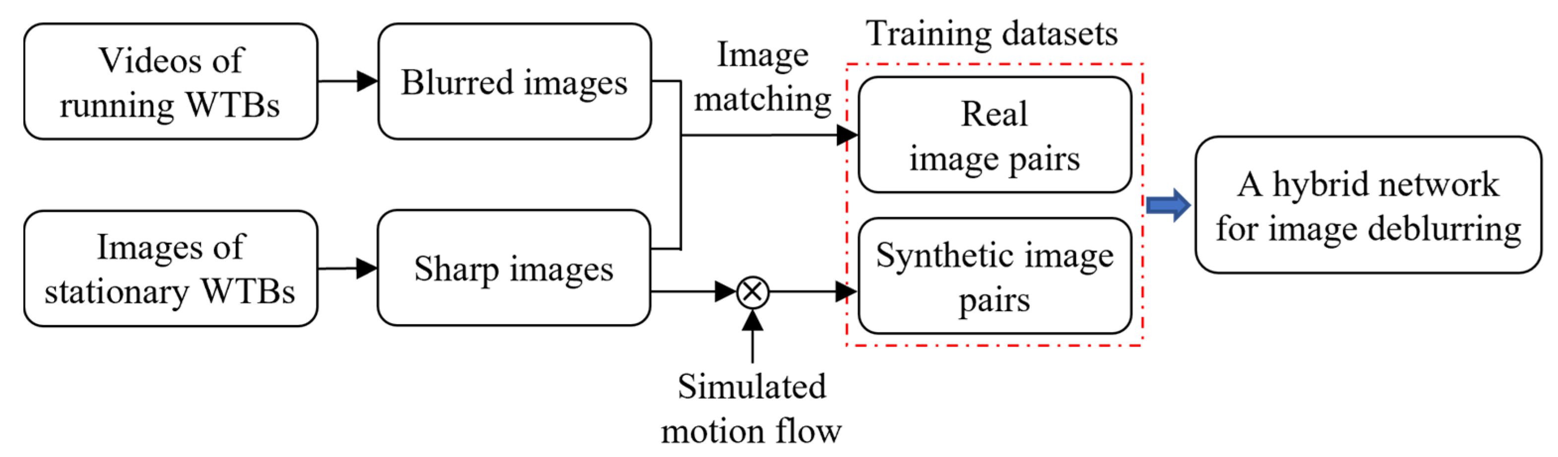
2. Synthetic Training Datasets

To train WTB image deblurring deep learning networks, image pairs, including blurred images and sharp images, have to be acquired. Although a 6D camera [24] and a high-speed camera such as the GoPro [21] can be used to clear images of a rotating target, their applications are limited because of the time-consuming processing and high cost of the hardware system. Meanwhile, the high-speed cameras cannot meet the requirement of WTB monitoring with various motion speeds. In comparison, simulation with clear images and blur kernel [20] can be applied in various motion scenes. Therefore, in our study, two strategies are employed to acquire the image pair samples. The first one is employed to capture image samples of the rotating blades using a digital camera; however, from different available methods, the clear images and their corresponding blur images are obtained using the image matching method. The second strategy is used to employ the sample synthesis method to prepare the image pair datasets of WTBs.

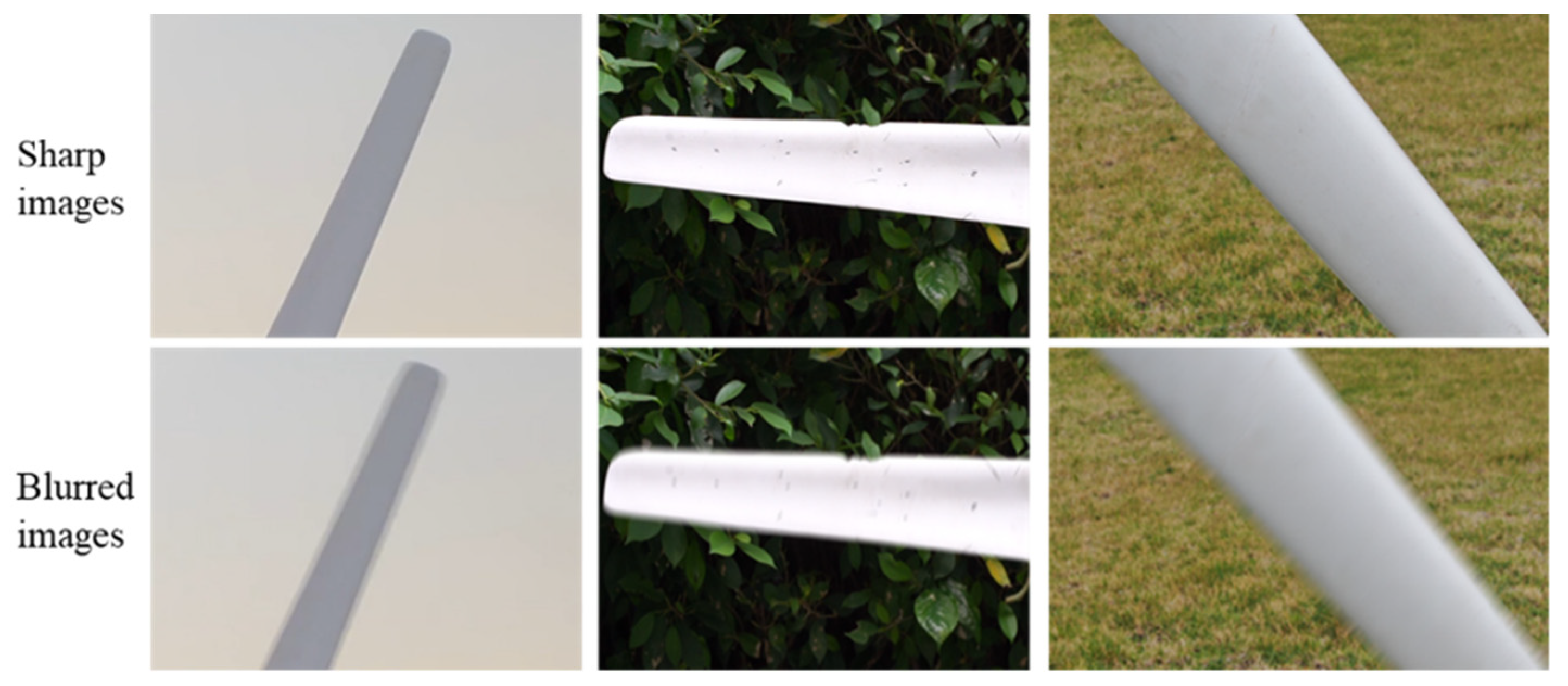
2.1. Image Pair Acquisition by Image Matching

The experimental site setup for image pair acquisition is shown in Figure 2. A high-performance UAV (e.g., DJI Mavic 2) and a digital camera (e.g., Sony A7M3) are used to capture the WTB images. During the imaging process, the UAV is controlled to fly stably, and the camera is fixed. Specifically, fine weather that has little influence on UAV image acquisition is necessary. Based on these working conditions, sharp images are captured from static WTBs. Then the WTBs are driven to rotate at different speeds, and the video of the rotating WTBs is captured with the same background. Blurred images are subsequently extracted from the video. Note that the sharp images are selected manually to ensure the image quality. In addition, the WTB motions are manually intervened to make the blades rotate in an exact orientation.
The sample acquisition process captured the sharp and blurred images in the same scene, and pairing is performed based on image matching, as shown in Figure 3. First, the sampled images are segmented using the Otus method [25] to separate the target blade regions from the image background. Different images in the blurred image sequence are obtained using image differences. Second, the difference image with the minimum difference is used to extract a blurred image to match the sharp image. Then, a sharp–blurred image pair with the same background is obtained. Note that image noise, shaking of the UAV camera, and minor changes in the environment could affect the image matching result. However, these influences can be suppressed by object segmentation and minimum image difference processing.
A dataset (dataset #1) containing five hundred image pairs is prepared using this method. Three examples are shown in Figure 4. The blades have two lengths of 810 mm and 1140 mm. The rotation speed of the blades is less than 7 rad/s. Videos in 2K-HD-format are captured using DJI Mavic2. The backgrounds include the sky, grass, walls, trees, etc. Videos are captured at 60 fps.

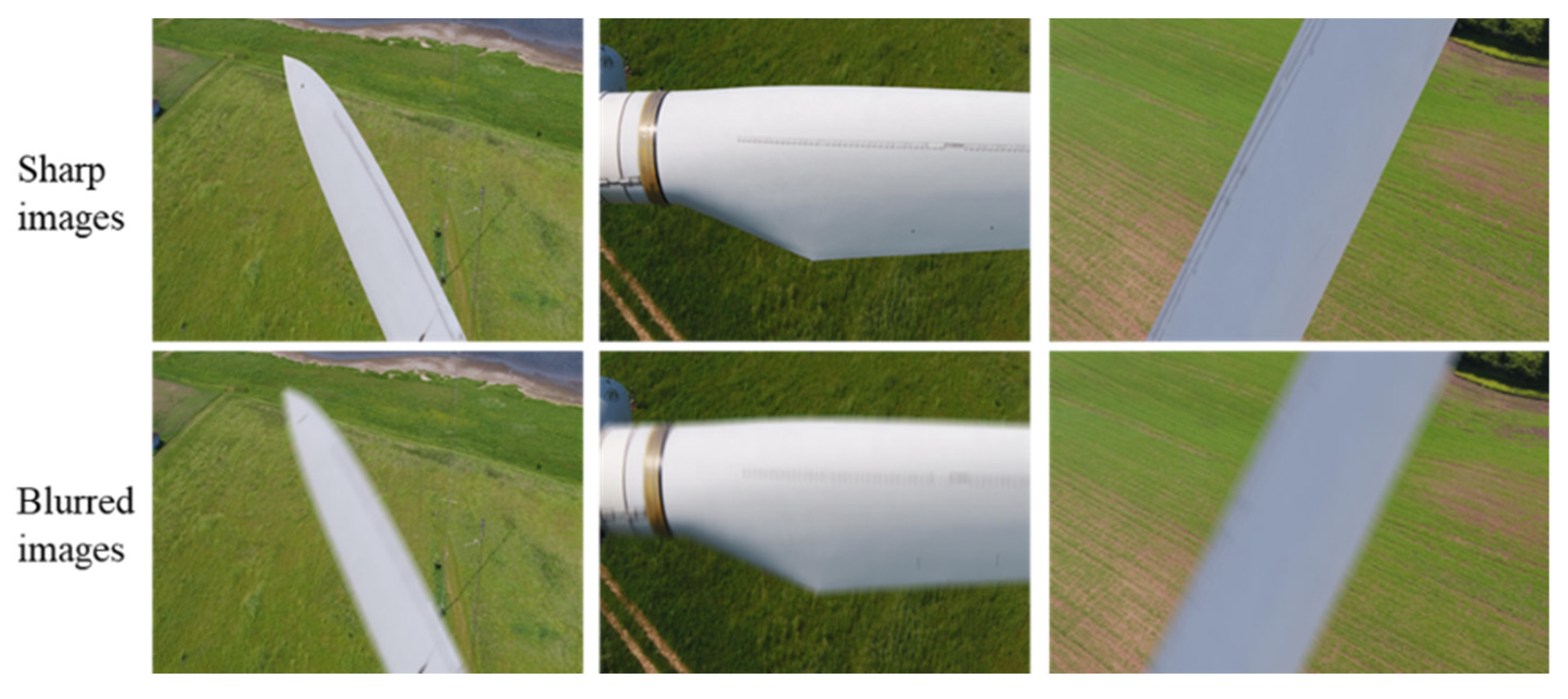
2.2. Image Pair Acquisition by Sample Synthesis

In practice, it is difficult to obtain WTB image pairs from different working conditions. To expand the datasets for training the motion deblurring network to improve generalization, two image pair datasets (dataset #2 and dataset #3) are synthesized. Using synthesis, continuous image frames are extracted from the videos and are fused to obtain the blurred images.
Dataset #2 synthesis: Clear image frames are continuously extracted from the video captured by a stationary high-speed camera. The corresponding blurred images are generated by averaging the image sequences. The Sony A7M3 (100 fps) and Iphone11 (240 fps) are used to capture videos of rotating WTBs. The rotation speed is less than 1 rad/s; 33,300 images are extracted from the videos. Blurred images are generated by averaging 20 consecutive image frames. Finally, a total of 1500 image pairs are synthesized using the captured video frames. Three examples are shown in Figure 5.
Dataset #3 synthesis: The rotation motion of WTBs is simulated, and the simulated motion flow data is merged into sharp images to produce the corresponding blurred images, as shown in Figure 6. The sharp images include the samples captured in Section 2.1 and are selected from public datasets, as shown in Figure 1, to simulate the practical applications in different scenes. Since relative motions occur between the WTB region and the camera, ROI segmentation is performed to extract the WTB region to eliminate the influence of the image background. Afterwards, the rotation motion of the WTB is simulated, and the simulated motion flow data is merged with the sharp images to produce blurred images.
The Otsu method is used to obtain the region of interest (ROI) mask of the WTB to extract the segmented image. Then, the WTB edge is obtained through morphological operations. A motion flow map containing rotation speed and direction is generated on the target region to simulate the WTB motion flow. The blur length and angle of the motion flow data are calculated using the blind deconvolution method reported in [20,26].
The schematic diagram of the motion flow simulation is shown in Figure 7. An x-y-z (Cartesian) coordinate system is located at the leftmost point of the ROI mask. The x-y plane is parallel to the imaging plane, and the z-axis is aligned and pointed away from the camera focal axis. To simplify the simulation process, the WTB angular velocity is assumed constant, and the motion plane is parallel to the imaging plane.
Hence, the motion scale s(i, j) and the motion angle θ(i, j) of the image pixel I(i, j) can be written as:
s ( i , j ) = ω ( i , j ) ( i c , j c ) 2
θ ( i , j ) = arctan [ ( j j c ) / ( i i c ) ]
where ω is the angular velocity of the WTB rotation motion. The rotation is regarded as clockwise when ω > 0 and is bounded by ||ω|| < 2 rad/s. Furthermore, ω can be replaced by its tangent value [20], that is:
s ( i , j ) = 2 tan ( ω / 2 ) ( i , j ) ( i c , j c ) 2
Since the simulated motion flow is parallel to the image plane, the direction of motion flow can be divided into vertical and horizontal components, and they are:
U ( i , j ) = s ( i , j ) cos ( π / 2 θ ( i , j ) )
V ( i , j ) = s ( i , j ) sin ( π / 2 θ ( i , j ) )
where U(i, j) and V(i, j) are the horizontal and vertical motions of pixel I(i, j), respectively. Based on the blind deconvolution method reported in [26], the kernel of the motion flow map (Km) is defined as:
K m = δ ( i sin θ + j cos θ ) / ( U ( i , j ) , V ( i , j ) ) 2
where δ(·) is the Dirac Delta function. Motion process is simulated by merging the motion kernel to sharp images (Is), and blurred images (IB) can be obtained as:
{ I b ( i , j ) = K m I s ( i , j ) + N ( i , j ) , i f   ( i , j ) I r o i ( i , j ) I b ( i , j ) = α ( K m I s ( i , j ) + N ( i , j ) ) + ( 1 α ) I s ( i , j ) , i f   ( i , j ) I e d g e ( i , j ) I b ( i , j ) = I s ( i , j ) , o t h e r w i s e  
where * denotes convolution operation, N is additive noise, α is a linear fusion factor; Iroi(i, j) and Iedge(i, j) represent the ROI mask and the target edge region. The pseudo-code of the synthesis processing is presented in Algorithm 1.
Algorithm 1 Blurred image synthesis
Operation: morphological dilation
      morphological erosion
      Dirac Delta function δ ( · )
Input: sharp image I s
   ROI mask I s r o i
   central point ( i c , j c )
   additive noise N is uniformed to (0, 0.5)
   morphological structuring element S e with size s
   angular velocity ω, ranging in (0, 2)
   linear fusion factor α
1: I d i l a t e I s r o i S e
2: I e d g e I d i l a t e I s r o i S e
3: K m 0
4: for each pixel ( i , j ) in I d i l a t e  do
5:   s ( i , j ) 2 t a n ( 2 / ω ) ( i , j ) ( i c , j c ) 2
6:   θ ( i , j ) arctan [ ( j j c ) / ( i i c ) ]
7:   U ( i , j ) s ( i , j ) c o s ( π / 2 θ ( i , j ) )
8:   V ( i , j ) s ( i , j ) sin ( π / 2 θ ( i , j ) )
9:  if  ( i , j ) 2 < ( U ( i , j ) , V ( i , j ) ) 2 / 2  then
10:    K m δ ( i sin ( θ ) + j cos ( θ ) ) / ( U ( i , j ) , V ( i , j ) ) 2
11:  end if
12: end for
13: for each pixel ( i , j ) in I s  do
14:  if  I s r o i ( i , j ) = = t r u e  then
15:    I B K m I s + N
16:  else if  I edge ( i , j ) = = t r u e  then
17:    I B α ( K m I s + N ) + ( 1 α ) I s
18:  else
19:    I B I s r o i
20: end if
21: end for
Output: blurred image I B
In this simulation stage, two thousand image pairs are synthesized using 701 images selected from the public dataset “DTU-Wind Turbine UAV Inspection Images” [12] to generate dataset #3. Three examples are shown in Figure 8 with the fusion factor α = 0.75 and the kernel size s = 5. Different rotating speeds are also synthesized.

3. Hybrid Motion Deblurring Network

As mentioned in the literature review, end-to-end networks such as DeepDeblur, DeblurGAN, and DeblurGANv2 are effective image motion deblurring models. DeblurGANv2 has better performance in accuracy and effectiveness. Hence, DeblurGANv2 is built to remove the motion blur from WTB images, and the process is shown in Figure 9. The model contains two sub-networks: the generator and the discriminator. The blurred images are used as the input, and the generator estimates the sharp images. The discriminato calculates the similarity between the restored images and the expected sharp images. The two sub-networks are updated based on their corresponding network loss values. The network loss, including the generator loss and the discriminator loss, is calculated using the RaGAN loss [23], the perceptual loss [27], and the mean square error (MSE) loss. After the model is trained, the generator is applied for image restoration, and the discriminator is frozen.

3.1. Generator

Inception-RestNet-v2 and MobileNet can be used to establish the generator of DeblurGANv2, which are respectively denoted as InceptionRestNetv2-DeblurGANv2 (I-DeblurGANv2) [23] and MobileNet-DeblurGANv2 (M-DeblurGANv2) [28]. Due to the higher accuracy, I-DeblurGANv2 is built for WTB image processing, and its generator structure is shown in Figure 10. The model can directly connect the input layers to the output layers through a residual network. The FPN includes 5 pooling layers, 18 convolutional layers, and 6 up-sampling layers, which consist of the bottom-top and top-down pathways. The bottom–top pathway is used to extract image features and compress the semantic context information. Then a top-down pathway is used to increase the spatial resolution of the output from the semantic layers. The cross-link between the bottom-top and top-down pathways provides high-resolution feature details that help detect and localize the target objects. In addition, the FPN model can achieve high processing efficiency from the multi-scale aggregation of extracted features.

3.2. Discriminator

The purpose of motion deblurring is to improve the image quality for automatic and precise WTBs inspection. Thus, it is necessary to obtain detailed information for surface damage detection. The receptive field of PatchGAN [29] focuses on the local interest regions of the input images; thus this network is used to establish the discriminator model, which prompts the generator to extract the image texture details.
Generally, the motion blur is unevenly distributed in a WTB image. The local blade regions must be identified using the discriminator to estimate the similarity of the restored images and the actual clear images. Thus, the discriminator is constructed as an eight-layer depth network to obtain a larger receptive field; the structure is shown in Figure 11. A sharp image and a restored image are used as the input; the network outputs the similarity values after the eight-layer convolutional operations. The step sizes of the first six and the last two convolution layers were set to 2 and 1, respectively.

3.3. Loss Function

The generator is designed to minimize the differences between restored images and sharp images. However, the embedded discriminator maximizes this difference. These operations may lead to gradient vanishing or explosions [30]. To address this problem, and because motion blur is produced mainly in the blade regions, a global discriminator is constructed to avoid network learning in local background areas. The RaGAN loss is used as the discriminator loss (Ld) to provide high-quality perceptual and clear outputs, and the loss is defined as [23]:
L d = E I s [ ( D ( I s ) E G ( I b ) D ( G ( I b ) ) 1 ) 2 ] + E G ( I b ) [ ( D ( G ( I b ) ) E I s D ( I s ) + 1 ) 2 ]
where D(·) is the discriminator output, G(·) is the generator output, and EIs and EG(Ib) are the expectation values of the probability distributions of Is and G(Ib).
For generator update, the MSE loss, discriminator loss, and perceptual loss are weighted to compose the generator loss function (Lg), that is:
L g = α 1 L m s e + α 2 L p + α 3 L d
where α 1 , α 2 and α 3 are weights that are usually set to 0.5, 0.006 and 0.01, respectively [23]. Lmse represents the mean square error of the generated image and the sharp image, LP represents the visual perception error [27] expressed by the L2 distance of the depth feature map between the generated image and the expected output image. Lmse and Lp are calculated by:
L m s e = 1 H W i = 1 H j = 1 W I s ( i , j ) G ( I b ( i , j ) ) 2
L p = 1 W 3 , 3 H 3 , 3 x = 1 W 3 , 3 y = 1 H 3 , 3 Φ ( I s ) ( x , y ) Φ ( G ( I b ) ) ( x , y ) 2
where W and H are the width and height of the input image, respectively; Φ ( · ) is the image feature map obtained from the third convolution layer of the VGG-19 network, which is trained using the ImgeNet samples [31]; W3,3 is the map width, and H3,3 is the map height.

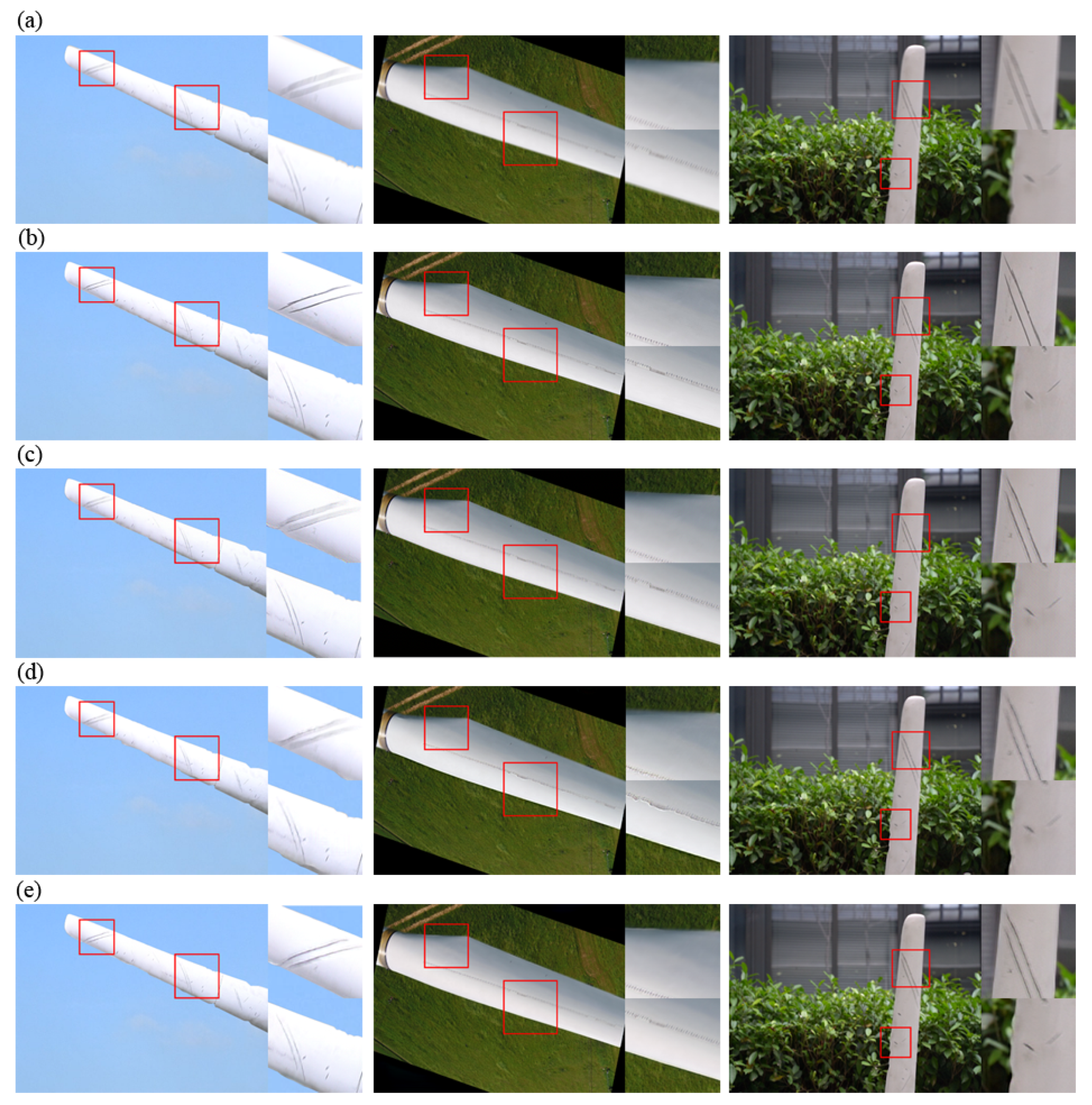
4. Experimental Results

Based on the process described in Section 2, three datasets containing 4000 synthetic image pair samples were acquired. Among these, the number of samples in 0–2 rad/s, 2–4 rad/s, and 4–7 rad/s are 2456, 979, and 565, respectively. In this work, 20% of all the samples are used as testing samples. In this case, only 113 image pairs in 4–7 rad/s are used for testing. Accordingly, 113 image pairs are selected from the image pairs in 0–2 rad/s, 2–4 rad/s as testing samples to ensure the sample balance. Therefore, a total of 339 image pairs were randomly chosen to test the network model; the remaining 3661 image pairs were used as the training samples. The image resolution of all image pairs is 600 × 800 pixels. The computer system used was an Intel Core i5-9400F CPU with 16 GB RAM, integrated with an NVIDIA GeForce GTX 1660 graphics card.
To evaluate the performance of motion deblurring networks, a comparative experiment was conducted using DeblurGAN [22], M-DeblurGANv2 [28], and I-DeblurGANv2 [23]. These three network models were trained in a single batch. The learning rate of the generator and the discriminator was initially set to 1Ee-4 and then reduced to zero during the training process. As the image restoration results are influenced by the rotation speed of the WTBs, the test samples were classified into three groups with rotational angular velocities of 0–2 rad/s, 2–4 rad/s, and 4–7 rad/s. Figure 12, Figure 13 and Figure 14 show the motion deblurring results of the three groups using the aforementioned three networks.
In Figure 12 and Figure 13, the images restored using I-DeblurGANv2 provide clearer and more detailed blade surface characteristics, including scratches, notches, cracks, and erosion marks. In Figure 14, more edge artefacts were generated in the restored images than in Figure 12 and Figure 13. Comparing the images in the third column in Figure 13 with the images in the second and third column in Figure 14, the DeblurGAN produces pseudo colors and artefacts on the WTB surfaces. In Figure 13d and Figure 14d, the blade edges were distorted from the M-DeblurGANv2 process. In contrast, I-DeblurGANv2 maintains clearer and smoother edges and texture information of the blade surfaces. Artefacts are difficult to avoid during motion deblurring. A higher degree of blur produces more artefacts. Thus, the image motion deblurring method has a limited application in WTB monitoring when the blade speed is higher than 7 rad/s.
The metrics of the peak signal-to-noise ratio (PSNR) and structural similarity index (SSIM) [32,33,34] were used to quantitatively measure the restoration effectiveness. A larger PSNR indicates that the restored image G(Ib) is closer to that of the sharp image Is. The SSIM ranges from 0 to 1. A larger SSIM indicates that the structure of G(Ib) is more similar to that of Is. PSNR and SSIM can be calculated from:
P S N R ( I s , G ( I b ) ) = 10 log 10 255 2 L m s e
S S I M ( I s , G ( I b ) ) = ( 2 μ S μ G + c 1 ) ( 2 σ S G + c 2 ) ( μ S 2 + μ G 2 + c 1 ) ( σ S 2 + σ G 2 + c 2 )
where μS and μG are the averages of Is and G(Ib), respectively; σS and σG represent the deviations of Is and G(Ib), respectively; σSG is the covariance of Is and G(Ib). c1 and c2 are constants usually set to 6.5025 and 58.5225, respectively [33].
Table 1 present the PSNR and SSIM values for G(Ib) with different rotational velocities. The I-DeblurGANv2 model produces the highest PSNR (80.138) and SSIM (0.950). The PSNR (86.128, 77.609, and 76.676) and SSIM (0.975, 0.940, and 0.908) with different rotational speeds obtained by the I-DeblurGANv2 are also the highest, indicating that the I-DeblurGANv2 model performs well in preserving object edge details, smoothness, and texture information, which are significant for WTB surface damage inspection.
The efficiencies of the three models were measured quantitatively (see Table 2). It can be seen that DeblurGAN has the lowest efficiency for image restoration (0.389 s). The processing time using I-DeblurGANv2 was 0.189 s, which is greater than that with M-DeblurGANv2 (0.105s). As shown in Table 2, the M-DeblurGANv2 model is a lightweight network that must operate 3.1 M parameters. The space consumption of the I-DeblurGANv2 model is 66.6 M parameters, leading to lower processing efficiency.

5. Discussion

Various blur scales and working in different scenes, including grassland, desert, mountain, and sea, are two main causes of difficulty and complexity for real-time WTB monitoring. For reliable and effective WTB inspection, different kinds of image pair samples with various blur scales are necessary to be captured in different scenes to train the proposed hybrid network to improve its generalization ability. It should be noted that clear and blur image pairs captured by digital cameras cannot be exactly matched because of dynamic environments. Accordingly, sample synthesis methods are more attractive to simulate the motion-blur WTB images. Image fusion algorithms and motion blur simulation can be combined together to acquire different kinds of image pairs.
It should also be noted that manual intervention is still required during image pair acquisition. First, sharp images are manually selected from the captured images using UAVs and digital cameras to guarantee the image quality. Second, the running motions of WTBs need to be controlled to make sure that the blurred images can be matched to the sharp images. Correspondingly, the human cost is an important problem to push forward this work. This also indicates that the generated datasets have great values for WTB monitoring.
With the available synthetic datasets, the proposed hybrid network, I-DeblurGANv2, provides high image quality both in PSNR and SSIM. This indicates that the proposed WTB image restoration model based on I-DeblurGANv2 is more suitable for maintaining detailed image information for WTB damage detection. In this study, the proposed method was verified to process blurred images sampled with a rotational velocity of less than 7 rad/s. Further research will be conducted to address blurred images with higher WTB rotation velocities. In addition, processing efficiency is also important for the real-time monitoring of running WTBs. However, a longer processing time (0.189 s of each image) is needed with our network than with M-DeblurGANv2 (0.105 s of each image). Therefore, the I-DeblurGANv2 model is necessary to be optimized by referencing a lightweight deep learning network to improve its efficiency.

6. Conclusions

In this study, we investigated the motion blur removal problem for UAV-based running WTBs images with the hybrid end-to-end network I-DeblurGANv2. A new large dataset including sharp-blurred image pairs of running WTBs was collected using a synthesis method. Specifically, three procedures were performed: (a) Blurred images were extracted from videos captured with rotational movement and matched to sharp images captured under static conditions based on minimizing the image difference; (b) Clear image frame sequences captured with a high-speed camera were used to produce synthetic blurred images; (c) The WTB movements were simulated to obtain motion flow parameters, and sharp images were synthesized with these parameters to produce blurred images. After the training and testing of the networks, the hybrid I-DeblurGANv2 model demonstrated better performance than the DeblurGANv2 and M-DeblurGANv2 models in terms of the PSNR and SSIM. This indicates that the proposed WTB image restoration model based on I-DeblurGANv2 is more suitable for maintaining detailed image information for WTB damage detection. It cannot be denied that our method behaves well at a little cost of time. Therefore, it is essential to investigate a more lightweight network framework that can be used for real-time WTB monitoring.

Author Contributions

Conceptualization, Y.P. and Z.T.; funding acquisition, Y.P., G.Z. and G.C.; methodology, Z.T.; validation, G.C. and C.W.; writing—original draft, Y.P. and Z.T.; writing—review and editing, Y.P. and G.Z.. All authors have read and agreed to the published version of the manuscript.

Funding

This research was funded by the National Natural Science Foundation of China (Grant Nos. 51905351, U1813212 and 61701123) and the Science and Technology Planning Project of Shenzhen Municipality, China (Grant No. JCYJ20190808113413430).

Conflicts of Interest

The authors declare no conflict of interest.

References

  1. Hasager, C.B.; Sjöholm, M. Editorial for the special issue “Remote Sensing of Atmospheric Conditions for Wind Energy Applications”. Remote Sens. 2019, 11, 781. [Google Scholar] [CrossRef] [Green Version]
  2. Li, Z.; Jiang, Y.; Guo, Q.; Hu, C.; Peng, Z. Multi-dimensional variational mode decomposition for bearing-crack detection in wind turbines with large driving-speed variations. Renew. Energy 2018, 116, 55–73. [Google Scholar] [CrossRef]
  3. Yang, R.; He, Y.; Zhang, H. Progress and trends in nondestructive testing and evaluation for wind turbine composite blade. Renew. Sustain. Energy Rev. 2016, 60, 1225–1250. [Google Scholar] [CrossRef]
  4. Ingersoll, B.; Ning, A. Efficient incorporation of fatigue damage constraints in wind turbine blade optimization. Wind Energy 2020, 23, 1063–1076. [Google Scholar] [CrossRef] [Green Version]
  5. Du, Y.; Zhou, S.; Jing, X.; Peng, Y.; Wu, H.; Kwok, N. Damage detection techniques for wind turbine blades: A review. Mech. Syst. Signal Process. 2020, 141, 106445. [Google Scholar] [CrossRef]
  6. Aird, J.A.; Quon, E.W.; Barthelmie, R.J.; Debnath, M.; Doubrawa, P.; Pryor, S.C. Region-based convolutional neural network for wind turbine wake characterization in complex terrain. Remote Sens. 2021, 13, 4438. [Google Scholar] [CrossRef]
  7. Movsessian, A.; García Cava, D.; Tcherniak, D. An artificial neural network methodology for damage detection: Demonstration on an operating wind turbine blade. Mech. Syst. Signal Process. 2021, 159, 107766. [Google Scholar] [CrossRef]
  8. Wang, B.; Lei, Y.; Li, N.; Wang, W. Multi-scale convolutional attention network for predicting remaining useful life of machinery. IEEE Trans. Ind. Electron. 2021, 68, 7496–7504. [Google Scholar] [CrossRef]
  9. Manso-Callejo, M.Á.; Cira, C.I.; Alcarria, R.; Arranz-Justel, J.J. Optimizing the recognition and feature extraction of wind turbines through hybrid semantic segmentation architectures. Remote Sens. 2020, 12, 3743. [Google Scholar] [CrossRef]
  10. Wang, L.; Zhang, Z.; Luo, X. A two-stage data-driven approach for image-based wind turbine blade crack inspections. IEEE/ASME Trans. Mechatron. 2019, 24, 1271–1281. [Google Scholar] [CrossRef]
  11. Wang, L.; Zhang, Z. Automatic detection of wind turbine blade surface cracks based on UAV-taken images. IEEE Trans. Ind. Electron. 2017, 64, 7293–7303. [Google Scholar] [CrossRef]
  12. Shihavuddin, A.; Chen, X.; Fedorov, V.; Nymark Christensen, A.; Andre Brogaard Riis, N.; Branner, K.; Bjorholm Dahl, A.; Reinhold Paulsen, R. Wind turbine surface damage detection by deep learning aided drone inspection analysis. Energies 2019, 12, 676. [Google Scholar] [CrossRef] [Green Version]
  13. Tao, Y.; Muller, J.-P. Super-resolution restoration of spaceborne ultra-high-resolution images using the UCL OpTiGAN system. Remote Sens. 2021, 13, 2269. [Google Scholar] [CrossRef]
  14. Wu, H.; Kwok, N.M.; Liu, S.; Li, R.; Wu, T.; Peng, Z. Restoration of defocused ferrograph images using a large kernel convolutional neural network. Wear 2019, 426–427, 1740–1747. [Google Scholar] [CrossRef]
  15. Szeliski, R. Computer Vision: Algorithms and Applications; Springer Science & Business Media: Berlin/Heidelberg, Germany, 2010. [Google Scholar]
  16. Fergus, R.; Singh, B.; Hertzmann, A.; Roweis, S.T.; Freeman, W.T. Removing camera shake from a single photograph. In ACM SIGGRAPH 2006 Papers; Siggraph: Boston, MA, USA, 2006; pp. 787–794. [Google Scholar]
  17. Zhang, H.; Wipf, D.; Zhang, Y. Multi-image blind deblurring using a coupled adaptive sparse prior. In Proceedings of the IEEE Conference on Computer Vision and Pattern Recognition, Portland, OR, USA, 23–28 June 2013; pp. 1051–1058. [Google Scholar]
  18. Gupta, A.; Joshi, N.; Zitnick, C.L.; Cohen, M.; Curless, B. Single image deblurring using motion density functions. In European Conference on Computer Vision; Springer: Berlin/Heidelberg, Germany, 2010; pp. 171–184. [Google Scholar]
  19. Sun, J.; Cao, W.; Xu, Z.; Ponce, J. Learning a convolutional neural network for non-uniform motion blur removal. In Proceedings of the IEEE Conference on Computer Vision and Pattern Recognition, Boston, MA, USA, 7–12 June 2015; pp. 769–777. [Google Scholar]
  20. Gong, D.; Yang, J.; Liu, L.; Zhang, Y.; Reid, I.; Shen, C.; Van Den Hengel, A.; Shi, Q. From motion blur to motion flow: A deep learning solution for removing heterogeneous motion blur. In Proceedings of the IEEE Conference on Computer Vision and Pattern Recognition, Honolulu, HI, USA, 21–26 July 2017; pp. 3806–3815. [Google Scholar]
  21. Nah, S.; Hyun Kim, T.; Mu Lee, K. Deep multi-scale convolutional neural network for dynamic scene deblurring. In Proceedings of the IEEE Conference on Computer Vision and Pattern Recognition, Honolulu, HI, USA, 21–26 July 2017; pp. 257–265. [Google Scholar]
  22. Kupyn, O.; Budzan, V.; Mykhailych, M.; Mishkin, D.; Matas, J. Deblurgan: Blind motion deblurring using conditional adversarial networks. In Proceedings of the IEEE Conference on Computer Vision and Pattern Recognition, Salt Lake City, UT, USA, 18–23 June 2018; pp. 8183–8192. [Google Scholar]
  23. Kupyn, O.; Martyniuk, T.; Wu, J.; Wang, Z. Deblurgan-v2: Deblurring (orders-of-magnitude) faster and better. In Proceedings of the IEEE International Conference on Computer Vision, Seoul, Korea, 27 October–2 November 2019; pp. 8877–8886. [Google Scholar]
  24. Köhler, R.; Hirsch, M.; Mohler, B.; Schölkopf, B.; Harmeling, S. Recording and playback of camera shake: Benchmarking blind deconvolution with a real-world database. In European Conference on Computer Vision; Springer: Berlin/Heidelberg, Germany, 2012; pp. 27–40. [Google Scholar]
  25. Otsu, N. A threshold selection method from gray-level histograms. IEEE Trans. Syst. Man Cybern. 1979, 9, 62–66. [Google Scholar] [CrossRef] [Green Version]
  26. Brusius, F.; Schwanecke, U.; Barth, P. Blind image deconvolution of linear motion blur. In International Conference on Computer Vision, Imaging and Computer Graphics; Springer: Berlin/Heidelberg, Germany, 2011; pp. 105–119. [Google Scholar]
  27. Johnson, J.; Alahi, A.; Li, F. Perceptual losses for real-time style transfer and super-resolution. In European Conference on Computer Vision; Springer: Berlin/Heidelberg, Germany, 2016; pp. 694–711. [Google Scholar]
  28. Howard, A.; Sandler, M.; Chen, B.; Wang, W.; Chen, L.; Tan, M.; Chu, G.; Vasudevan, V.; Zhu, Y.; Pang, R.; et al. Searching for mobilenetv3. In Proceedings of the IEEE International Conference on Computer Vision, Seoul, Korea, 27 October–2 November 2019; pp. 1314–1324. [Google Scholar]
  29. Isola, P.; Zhu, J.; Zhou, T.; Efros, A.A. Image-to-image translation with conditional adversarial networks. In Proceedings of the IEEE Conference on Computer Vision and Pattern Recognition, Honolulu, HI, USA, 21–26 July 2017; pp. 1125–1134. [Google Scholar]
  30. Salimans, T.; Goodfellow, I.; Zaremba, W.; Cheung, V.; Radford, A.; Chen, X. Improved techniques for training gans. arXiv 2016, arXiv:1606.03498. [Google Scholar]
  31. Deng, J.; Dong, W.; Socher, R.; Li, L.; Li, K.; Li, F. Imagenet: A large-scale hierarchical image database. In In Proceedings of the 2009 IEEE Conference on Computer Vision and Pattern Eecognition, Miami, FL, USA, 20–25 June 2009; pp. 248–255. [Google Scholar]
  32. Li, G.; Yang, Y.; Qu, X.; Cao, D.; Li, K. A deep learning based image enhancement approach for autonomous driving at night. Knowl. Based Syst. 2021, 213, 106617. [Google Scholar] [CrossRef]
  33. Wang, Z.; Bovik, A.C.; Sheikh, H.R.; Simoncelli, E.P. Image quality assessment: From error visibility to structural similarity. IEEE Trans. Image Process. 2004, 13, 600–612. [Google Scholar] [CrossRef] [PubMed] [Green Version]
  34. Li, G.; Lin, Y.; Qu, X. An infrared and visible image fusion method based on multi-scale transformation and norm optimization. Inf. Fusion 2021, 71, 109–129. [Google Scholar] [CrossRef]
Figure 1. Flowchart of the dataset synthesis process.
Remotesensing 14 00087 g001
Figure 2. Image pair acquisition setup: (a) Imaging with a stably controlled UAV; (b) Imaging with a fixed camera.
Remotesensing 14 00087 g002
Figure 3. Image pair acquisition by image matching.
Remotesensing 14 00087 g003
Figure 4. Three example images from dataset #1.
Remotesensing 14 00087 g004
Figure 5. Three example images from dataset #2.
Remotesensing 14 00087 g005
Figure 6. The image pair synthesis process.
Remotesensing 14 00087 g006
Figure 7. Schematic diagram of the motion flow simulation.
Remotesensing 14 00087 g007
Figure 8. Three example images from dataset #3.3. Hybrid Motion Deblurring Network.
Remotesensing 14 00087 g008
Figure 9. Flowchart of DeblurGANv2-based motion deblurring of WTB images.
Remotesensing 14 00087 g009
Figure 10. I-DeblurGANv2 generator structure.
Remotesensing 14 00087 g010
Figure 11. Discriminator structure.
Remotesensing 14 00087 g011
Figure 12. Motion deblurring results for images captured with a rotational angular velocity of 0–2 rad/s (the blur length increases from left to right column): (a) Blurred images; (b) Sharp images; (c) Restored images using the DeblurGAN; (d) Restored images using the M-DeblurGANv2; (e) Restored images using the I-DeblurGANv2.
Remotesensing 14 00087 g012
Figure 13. Motion deblurring results for images captured with a rotational angular velocity of 2–4 rad/s (the blur length increases from left to right column): (a) Blurred images; (b) Sharp images; (c) Restored images using the DeblurGAN; (d) Restored images using the M-DeblurGANv2; (e) Restored images using the I-DeblurGANv2.
Remotesensing 14 00087 g013
Figure 14. Motion deblurring results for images captured with a rotational angular velocity of 4–7 rad/s (the blur length increases from left to right column): (a) Blurred images; (b) Sharp images; (c) Restored images using the DeblurGAN; (d) Restored images using the M-DeblurGANv2; (e) Restored images using the I-DeblurGANv2.
Remotesensing 14 00087 g014
Table 1. PSNR and SSIM of G(Ib) with different rotational velocities.
Network ModelPSNRSSIM
0–2 rad/s2–4 rad/s4–7 rad/sAverage0–2 rad/s2–4 rad/s4–7 rad/sAverage
DeblurGAN80.92274.17972.35575.8190.9530.8460.7660.855
M-DeblurGANv285.17976.87175.52379.1910.9750.9320.8960.934
I-DeblurGANv286.12877.60976.67680.1380.9750.9400.9080.950
Table 2. Efficiency of the three models.
Network ModelNumber of ParametersAverage Running Time
DeblurGAN11.7 M0.389 s
M-DeblurGANv23.1 M0.105 s
I-DeblurGANv266.6 M0.189 s
Publisher’s Note: MDPI stays neutral with regard to jurisdictional claims in published maps and institutional affiliations.

