Article

Red Tide Detection Method for HY−1D Coastal Zone Imager Based on U−Net Convolutional Neural Network

1
College of Geodesy and Geomatics, Shandong University of Science and Technology, Qingdao 266590, China
2
First Institute of Oceanography, Ministry of Natural Resources, Qingdao 266061, China
3
Technology Innovation Center for Ocean Telemetry, MNR, Qingdao 266061, China
4
National Satellite Ocean Application Service, Beijing 100081, China
*
Author to whom correspondence should be addressed.
Remote Sens. 2022, 14(1), 88; https://doi.org/10.3390/rs14010088
Submission received: 9 November 2021 / Revised: 16 December 2021 / Accepted: 22 December 2021 / Published: 25 December 2021
(This article belongs to the Special Issue Remote Sensing for Monitoring Harmful Algal Blooms)

Abstract

:
Existing red tide detection methods have mainly been developed for ocean color satellite data with low spatial resolution and high spectral resolution. Higher spatial resolution satellite images are required for red tides with fine scale and scattered distribution. However, red tide detection methods for ocean color satellite data cannot be directly applied to medium–high spatial resolution satellite data owing to the shortage of red tide responsive bands. Therefore, a new red tide detection method for medium–high spatial resolution satellite data is required. This study proposes the red tide detection U−Net (RDU−Net) model by considering the HY−1D Coastal Zone Imager (HY−1D CZI) as an example. RDU−Net employs the channel attention model to derive the inter−channel relationship of red tide information in order to reduce the influence of the marine environment on red tide detection. Moreover, the boundary and binary cross entropy (BBCE) loss function, which incorporates the boundary loss, is used to obtain clear and accurate red tide boundaries. In addition, a multi−feature dataset including the HY−1D CZI radiance and Normalized Difference Vegetation Index (NDVI) is employed to enhance the spectral difference between red tides and seawater and thus improve the accuracy of red tide detection. Experimental results show that RDU−Net can detect red tides accurately without a precedent threshold. Precision and Recall of 87.47% and 86.62%, respectively, are achieved, while the F1−score and Kappa are 0.87. Compared with the existing method, the F1−score is improved by 0.07–0.21. Furthermore, the proposed method can detect red tides accurately even under interference from clouds and fog, and it shows good performance in the case of red tide edges and scattered distribution areas. Moreover, it shows good applicability and can be successfully applied to other satellite data with high spatial resolution and large bandwidth, such as GF−1 Wide Field of View 2 (WFV2) images.

1. Introduction

Red tides refer to harmful algal blooms (HABs) that constitute a marine ecological disaster resulting from excessive reproduction or accumulation of plankton, protozoa, or bacteria that cause water discoloration [1,2]. Red tide outbreaks are a threat to fisheries, marine ecosystems, and human health [3,4,5,6]. The dominant phytoplankton which caused red tide in China include dinoflagellates (such as Noctilucent scintillans [7], Prorocentrum donghaiense (P. donghaiense) [8], Alexandrium catenella [9]), and diatom (such as Skeletonema costatum (S. coatatum) [10]). In recent years, red tides have been found to occur more frequently as a result of eutrophication [11,12,13,14]. According to statistics, in 2019 alone, a total of 38 large−scale red tides occurred in China, resulting in direct economic losses of up to USD 4.86 million [15]. Automatic detection and monitoring of red tides is important for red tide prevention and reduction.
Red tide detection and monitoring methods include in situ surveys and remote sensing [16]. Owing to its wide range and short revisit period, remote sensing technology has played an important role in red tide detection and monitoring [17,18,19]. Multiple ocean color satellites, including the Coastal Zone Color Scanner (CZCS, NASA), Sea−Viewing Wide Field–of–View Sensor (SeaWiFs, NASA), Moderate Resolution Imaging Spectroradiometer (MODIS, NASA), Visible and Infrared Imager Radiometer Suite (VIIRS, NASA), Medium Resolution Imaging Spectrometer (MERIS, ESA), and Geostationary Ocean Color Imager (GOCI, South Korea), have been used for red tide detection and monitoring. However, the spatial resolution of such ocean color satellite data is too low (>250 m) to detect red tides with fine scale and scattered distribution [20]. Therefore, remote sensing images with medium–high resolution have been increasing in use in red tide detection [21]. In recent years, China has launched a series of remote sensing satellites with medium–high resolution. For example, HY−1D, China’s fourth ocean optical satellite, was launched in June 2020. The CZI onboard HY−1D, with a spatial resolution of 50 m, wide swaths of 950 km, and a revisit period of 3 days, has been increasingly used for monitoring marine disasters including red tides.
Most existing red tide detection methods based on spectral features have been developed for ocean color satellites, such as the red tide index (RI) [22], P. donghaiense index (PDI), and diatom index (DI) [23], as well as a series of improved RI algorithms [24,25]. Of these, the RI is calculated by three bands at 443, 510, and 555 nm. PDI and DI utilize the 443, 510, and 555 nm bands and the 488, 531, and 555 nm bands, respectively. Studies have also attempted to use the chlorophyll−a concentration, bio−optical properties of seawater, or fluorescence line height (FLH) as alternative indicators of red tides [26,27,28]. However, due to without corresponding bands, these red tide monitoring methods cannot be directly applied to remote sensing satellite data with medium–high spatial resolution, such as HY−1D CZI images for limited bands (R, G, B, and NIR) and broad bandwidth. Some red tide detection algorithms have been developed for remote sensing satellites with medium–high spatial resolution. For example, the spectral shape at 490 nm from multiple sensor data, including Sentinel−2 MSI and Landsat OLI, was used by Shin et al. [29] to detect red tides of M. polykrikoides near the Korean Peninsula with high performance. Liu et al. [20] proposed a red tide detection algorithm (GF1_RI algorithm) for broad band satellite data with high spatial resolution using GF−1 WFV data, which was successfully applied to the red tide of Noctilucent scintillans detection and monitoring in Guangdong and Shandong provinces, China. These studies verified the red tide detection capability of images with medium–high spatial resolution with broad bandwidth. However, the aforementioned methods usually require a predetermined threshold to diagnose red tides effectively, and the selection of the threshold is strongly region−dependent and susceptible to the marine environment. For example, the threshold may be invalid when the image is contaminated by clouds, sun glint, or aerosols. Therefore, it is necessary to develop an automatic red tide detection method for images with medium–high spatial resolution without a threshold.
Deep learning [30] has been widely used in remote sensing applications such as remote sensing image classification [31,32,33], target recognition [34,35], and image fusion [36]. Owing to its powerful large data mining and feature extraction capabilities [37], deep learning has also been applied to red tide detection with good results. Most existing red tide detection methods based on deep learning use hyperspectral images [38,39], synthetic dataset based Inherent Optical Properties (IOP) combinations [40], and in situ data [41], which have rich red tide features and response bands. However, owing to the low spectral resolution, the spectral information of satellite data with medium–high spatial resolution is not as rich as that of hyperspectral data. As a nonlinear method with powerful data mining capability, deep learning is expected to extract more red tide features from satellite data with medium–high spatial resolution and detect red tide ranges more accurately. Considering the red tide of Noctilucent scintillans that occurred in the East China Sea in August 2020 which reported by the National Satellite Ocean Application Service (NSOAS) as an example, this study proposes an advanced red tide detection method based on the U−Net model, namely RDU−Net.
The remainder of this paper is organized as follows. Section 2 introduces the satellite data and related methodology. Section 3 presents the proposed method, namely RDU−Net, and the experimental results. Section 4 discusses the effects of the loss function coefficients and input characteristics on the proposed model. Finally, Section 5 concludes the paper.

2. Materials and Methods
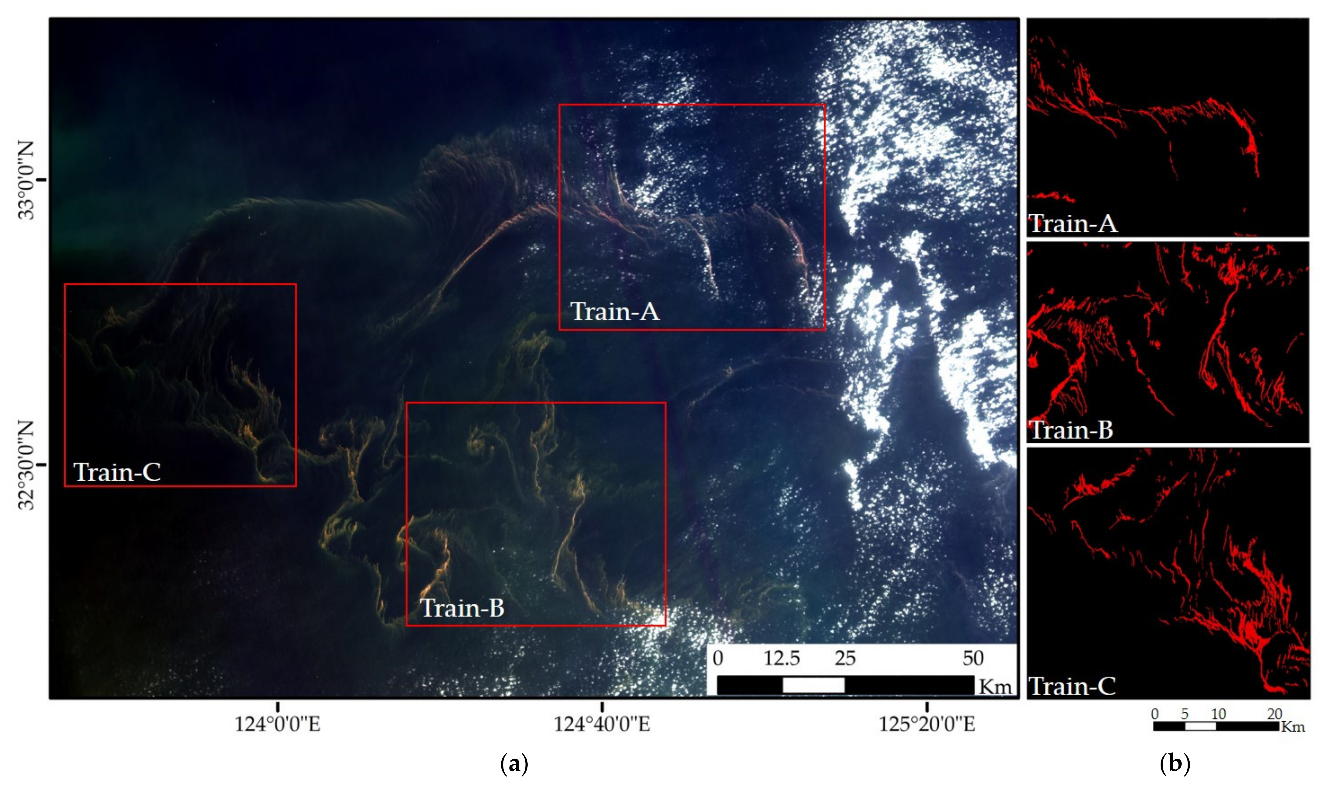
2.1. Satellite Data

Noctilucent scintillans red tide occurred in the East China Sea in August 2020, as reported by the National Satellite Ocean Application Service (NSOAS) [42] (Figure 1a). The HY−1D CZI Level−1B data (Figure 1b) imaged during this red tide were acquired from NSOAS. The CZI characteristics are summarized in Table 1. Compared with ocean color satellites with spatial resolution >250 m, HY−1D CZI has an obvious advantage owing to its spatial resolution of 50 m. Furthermore, CZI has the advantages of wide swaths (950 km) and a short revisit period (3 days). Therefore, CZI has been widely used in marine monitoring.
To explore the applicability of the proposed method, GF−1 Wide Field of View (WFV) data were acquired from China’s Center for Resource Satellite Data and Application (CRESDA) [43] in this study. As a representative Chinese high−resolution satellite, the GF−1 with four WFV cameras was launched in 2013. GF−1 WFV also has the advantage of high spatial resolution (16 m), wide scene swaths (800 km), and a short revisit period (4 days). Therefore, GF−1 WFV images are often used in marine monitoring. The sensor characteristics of GF−1 WFV [44] are summarized in Table 1. The GF−1 WFV2 Level−1 data are shown in Figure 1c. The detailed information of the two images is summarized in Table 2.

2.2. Dataset Construction

Considering the distribution characteristics of different objects in the study area, three areas were selected when constructing the training sample dataset, as shown in Figure 2. The true values (Figure 2b) were obtained on the basis of visual interpretation. Moreover, considering the computer memory and speed, the input sample size of the model was set to 256 × 256. Therefore, the images and corresponding labels were randomly divided into sample images with a size of 256 × 256 pixels. A total of 680 samples were generated. Furthermore, three types of data augmentation were adopted to obtain sufficient training data and avoid overfitting, including horizontal flip, vertical flip, and diagonal flip. Therefore, a dataset containing 2720 samples was established and randomly divided into training (80%) and validation (20%) datasets.

2.3. Related Methodology

2.3.1. U−Net Model

U−Net is an improved fully convolutional network proposed in 2015 by Ronneberger et al. [45] for the semantic segmentation of biomedical images. U−Net has been widely used in medical diagnosis [46,47], remote sensing [48], and other fields [49,50] as a pixel−wise prediction model that can be trained in an end−to−end manner. Owing to context−based learning, U−Net can propagate context information to higher resolution layers to build high level features for precise detection. Moreover, U−Net can support image segmentation with a few samples. Therefore, research on red tide detection has been carried out on the basis of the U−Net model.
The structure of U−Net is mainly divided into an encoder and a decoder, which can be represented by a U−shaped diagram. Unlike a general convolutional network, U−Net does not have any fully connected layers and uses only the valid part of each convolution. The encoder path is also known as the contracting path. It is used to extract features from the input image following the typical architecture of a convolutional network. It consists of five blocks, each of which includes two convolutions (unpadded convolutions), an activation function, and a max pooling layer for down−sampling. In each block of the encoder, the receptive field size is increased, the output size is halved, and the number of feature channels is doubled. The decoder path is also known as the expansion path. It consists of up−convolutions and concatenations with features from the contracting path. Every block in the decoder path consists of an up−sampling, a concatenation with the correspondingly cropped feature map from the contracting path, and two convolutions, each followed by an activation function. The output of the decoder path consists of the category and localization, i.e., a category label (red tide or not) is assigned to each pixel.

2.3.2. Comparison Methods

For comparison, three convolutional neural networks (including U−Net), a machine learning method (SVM), and a spectral ratio method (GF1_RI) are selected in this study. The details of each algorithm are as follows:
(1) Fully Convolutional Neural Networks (FCN)
The fully convolutional neural network (FCN) [51] has achieved good results. It adopts the skip architecture to combine semantic information from a deep, coarse layer with appearance information from a shallow, fine layer in order to produce accurate and detailed segmentations. A series of networks developed on the basis of FCN have confirmed its strong generalization ability [52]. FCN includes three networks: FCN−32s, FCN−16s, and FCN−8s.
FCN−8s is an advanced version of FCN−32s and FCN−16s, and it outperforms FCN−16s and FCN−32s in image segmentation. Thus, FCN−8s was selected for comparative experiments. Furthermore, FCN−8s does not have fully connected layers. The classification at the image label is extended to the pixel label by modifying fully connected layers into convolutional layers.
(2) SegNet
SegNet [53] is a deep network for image semantic segmentation, which is similar to FCN. SegNet was designed for scene segmentation with high learning speed and accuracy using a highly unbalanced dataset [46]. The dataset used in this study was also unbalanced. Hence, SegNet was chosen for comparison. The architecture of SegNet consists of encoder and decoder processes. The encoder process involves image compression and feature extraction using the rectified linear unit (ReLU) [54] during activation. Upon its completion, the decoder process restores the image. Image spatial information is maintained during the decoder process, as image restoration is performed using the same pooling layer as that in the encoder process. This feature of SegNet distinguishes it from FCN. When the image reconstruction is complete, the image is classified using a softmax function [47]. Compared with the corresponding structure of FCN, the volume of SegNet is much smaller mainly because of the operation performed by SegNet to balance the computational effort: the location information of the recorded pooling process is used instead of a direct deconvolution operation.
(3) SVM
SVM is a kernel−based supervised classification algorithm proposed by Cortes and Vapnik [54]. It has been shown to be a powerful machine learning algorithm for pattern recognition and nonlinear regression, and it is mainly used for classification, regression, and time−series prediction [55,56]. The basic idea of SVM is to find the optimal hyperplane that can correctly partition the training dataset with the maximum geometric spacing, as follows:
f X i = i = 1 N W i φ X i + b
where φ(Xi) is the nonlinear mapping function, and Wi and b are the linear support vector regression function parameters.
The common kernel functions in SVM include the linear kernel, polynomial kernel, and Gaussian kernel [57]. Among them, only the Gaussian kernel needs to adjust its parameters to achieve the best performance. The parameters of the Gaussian kernel function include the penalty factor c and kernel width γ. Smaller values of c and γ will increase the training error, while larger values will increase the complexity of the model and lead to overfitting. In this study, the optimal parameters of the model were c = 2.0 and γ = 4.0.
(4) GF1_RI
GF1_RI is a red tide detection method for GF−1 WFV images proposed by Liu [20] according to the spectral characteristics of red tides. The clouds, turbid water, and construction regions in the image are first masked according to the spectrum of blue and green bands; then, the red tide area is detected using the GF1_RI index as follows:
G F 1 _ R I = L 3 ( L 2 + L 4 ) / 2
where L2, L3, and L4 represent the radiance values of the green, red, and NIR bands, respectively.

2.3.3. Accuracy Evaluation

The performance of the proposed method was evaluated using four criteria, including Precision, Recall, F1−score, and Kappa. Precision is the ratio of red tide pixels accurately detected to all red tide pixels identified. Recall represents the percentage of pixels classified as red tides that are correctly classified. F1−score is an indicator of the accuracy of the red tide detection method, which combines precision and recall. The kappa coefficient is a type of accuracy evaluation index used to measure the consistency of the red tide detection results with greater objectivity. The calculation methods are given below:
P r e c i s i o n = T P T P + F P × 100 %
R e c a l l = T P T P + F N × 100 %
F 1 s c o r e = 2 × P r e c i s s i o n × R e c a l l P r e c e s s i o n + R e c a l l
K a p p a = T P + T N T N + F P × T N + F N + F N + T P × F P + T P
where TP and FP denote the true positive and false positive, i.e., the number of red tide and non−red tide pixels identified as red tide, respectively; FN denotes the false negative, i.e., the number of red tide pixels identified as non−red tide; and TN denotes the true negative, i.e., the number of non−red tide pixels correctly identified as non−red tide.

3. RDU−Net Model for Red Tide Detection

3.1. RDU−Net Model Framework

Owing to limitations in terms of the bands and spectral resolution, red tide detection for satellite images with medium–high resolution requires strong feature representations, especially for red tides with fine scale and scattered distribution. In addition, U−net is not effective in extracting detailed information of red tides [58], such as the red tide boundary. Therefore, RDU−Net is proposed by incorporating channel attention and improving the loss function on the basis of traditional U−Net. Furthermore, some layers are also added in RDU−Net to improve the training performance. The batch normalization (BN) layer [59] can achieve a stable distribution of activation values throughout training, thereby accelerating the model convergence and increasing the model capacity. Moreover, to make the output image size consistent with the input image size, the same strategy is adopted to replace the valid part in the padding. In addition, as the model training in this study is based on a small training set, a dropout layer is added before up−sampling to avoid overfitting. This design retains the information lost by down−sampling to a certain extent.
The RDU−Net model framework is shown in Figure 3.

3.1.1. Channel Attention Model

Red tides have different spectral characteristics in different bands (channels). Mining the inter−channel features can facilitate red tide information detection. However, the convolutional layer extracts feature by blending cross−channel and spatial information together [60,61]. In recent years, the attention model has also been widely used in deep learning networks to improve the performance. Channel attention can automatically obtain valuable features by learning and exploring the inter−channel relationships. Therefore, this study uses channel attention to generate the channel attention map by exploring the characteristic relationship between channels, and greater attention is paid to the red tide formation between different channels.
The channel attention module integrates MaxPool and AvgPool to enrich the extracted high−level features and considerably improve the representation capability of the network. The channel attention framework is shown in Figure 4.
The channel attention module can be expressed as follows:
F C A = F F M σ M L P F M P M L P F A P
where FFM denotes the feature map from the convolution block and FCA denotes the channel attention map; FMP and FAP represent the feature map obtained by the MaxPool and AvgPool operations, respectively; σ denotes the activation function; and ⊕, ⊗ denote element addition and multiplication, respectively.
First, two feature maps are obtained by applying the MaxPool and AvgPool operations to the input features. Second, the two maps are input to the multi−layer perceptron (MLP) with one hidden layer. Third, the output feature vectors are merged and activated by the element−wise summation and activation function. Finally, the channel attention map is obtained by multiplying the output feature vectors by the feature map obtained by the convolution block.

3.1.2. Boundary and Binary Cross Entropy Loss Function

For unbalanced red tide samples, i.e., when the number of positive (red tide) and negative samples (background) varies considerably, using only the loss function based on the regional integrals can affect the performance of model training and red tide boundary detection [62]. The boundary loss function can alleviate the difficulty arising from unbalanced red tide samples. Therefore, to achieve red tide edge detection with greater accuracy and clarity, the boundary and binary cross entropy (BBCE) loss function, which combines the boundary and region information, was chosen in this study.
The boundary loss function [63] is proposed by calculating the distance between the boundaries in a differentiable form:
D i s t G , S = 2 Δ S D G q d q
where G and S are two nearby regions; ∂G and ∂S are boundaries of G and S; ∆S represents the region between ∂G and ∂S; and DG(q) denotes the distance between any point q and the nearest point on ∂G.
Subsequently, the sum of the region integrals represented by the boundary−based level set ϕG is calculated, and the final loss value is obtained by outputting the binary variables Sθ(q) through the softmax probability of the network as follows:
L B θ = Ω ϕ G q   s θ q d q
In this study, the BCE loss function is used to measure the loss value of the region as follows:
L B C E = 1 N n = 1 N w [ y n log x n + 1 y n log 1 x n ]
where w is a hyper−parameter, and x and y are the predicted result and true label, respectively. By incorporating the boundary loss, the loss function LBBCE makes the training consider the accuracy of the boundary:
L B B C E = α L B C E + ( 1 α ) L B
where α is an arbitrary weight belonging to [0, 1].

3.2. Flowchart of Red Tide Detection Based on RDU−Net Model

Figure 5 shows the overall flowchart of the proposed method.

3.2.1. Data Preprocessing

Data preprocessing includes geometric correction, feature combination, and data normalization. In this study, we used ENVI 5.3 software to perform geometric correction.
High−resolution remote sensing images contain more intricate details and texture information. However, owing to the limitation of band configuration, it is difficult to distinguish features (such as turbid water) similar to red tides. Moreover, the separability of the spectral information of red tides and seawater is weak at the red tide edges. From the spectral curves of the selected samples, it can be seen that the red tides respond strongly in the red and NIR bands. Therefore, NDVI was introduced to enhance the spectral information of red tides. NDVI is calculated as:
N D V I = R ( N I R ) R ( R ) R ( N I R ) + R ( R )
where R(NIR) and R(R) denote the radiance values of the near−infrared and red bands, respectively. As shown in Figure 6b, the statistics results show that the NDVI of red tides is significantly different from that of other objects such as seawater. Therefore, NDVI is taken as the input feature in this study. The average NDVI values were all less than 0, among which that of seawater was the lowest with the minimum variance, followed by red tides. By using the multi−feature multispectral data, which combines the original multispectral data (four bands) and NDVI, high level information can be extracted. The spatial information of seawater is suppressed, and the spectral differences between red tides and seawater are increased.
To unify the dimensions of multiple features, the maximum and minimum value normalization method [64] was adopted to normalize the gray value of the preprocessed image and samples to [0, 1]. The algorithm is given by:
x = x x min x max x min
where x* represents the normalized vector, x is the sample spectral vector, and xmax and xmin are the maximum and minimum values of the sample spectral vector, respectively.

3.2.2. Splicing Method Based on Ignoring Boundary
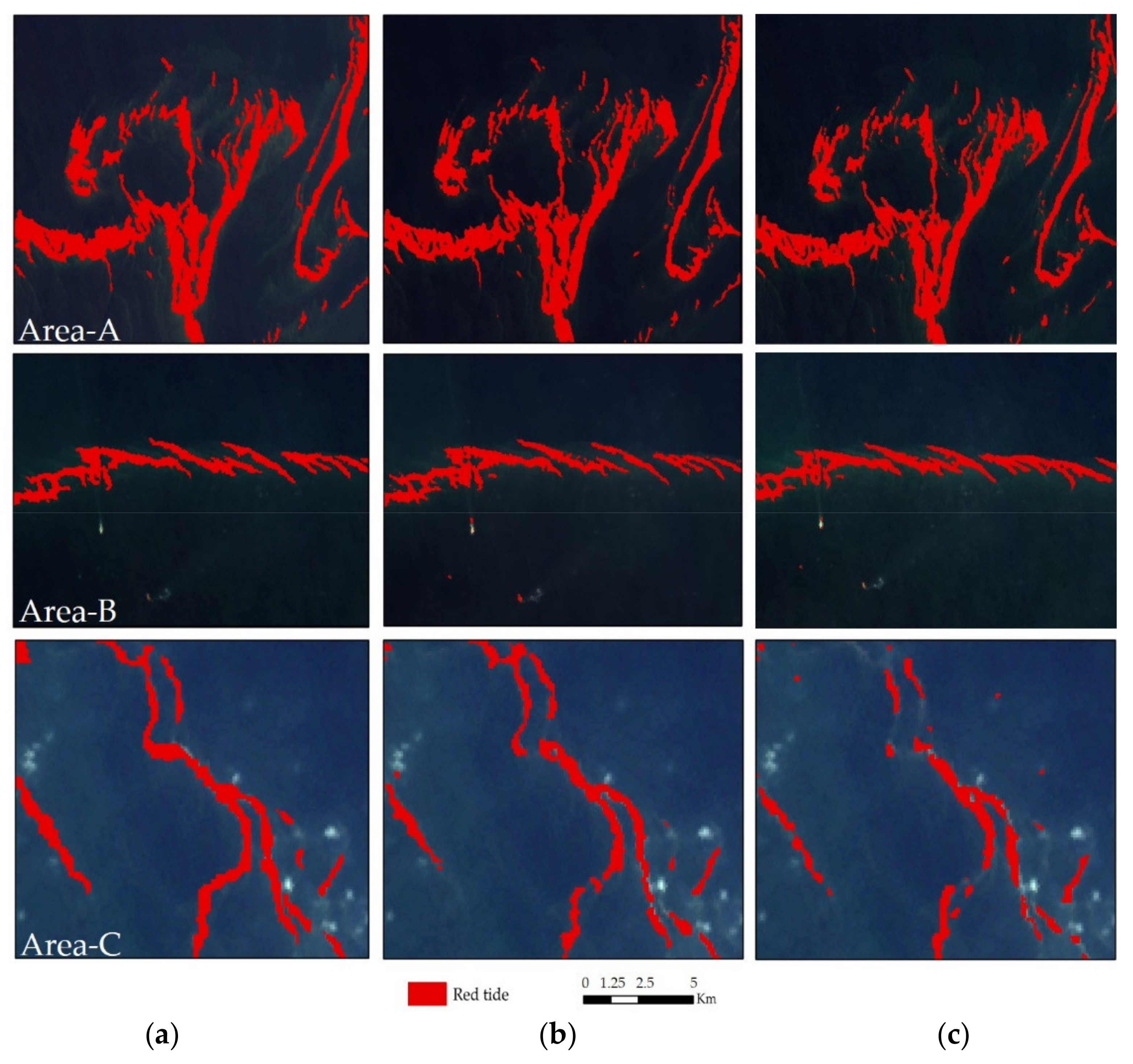
Splicing method based on ignoring boundary is used to avoid the obvious stitching marks. Following steps were performed to achieve the detection of the red tide.
Step 1: Calculate the step size of image cropping by setting the ratio of the splicing area to the input area. The formula is as follows.
s = n × O L _ r a t i o
where s represents the step size during image cropping, OL_ratio represents the ratio of the splicing area to the input area, and n represents the width of the image block. In this paper, the OL_ratio is set to 50%, and n takes 256 pixels.
Step 2: The whole image was cropped into a series of image blocks with a size of n × n according to the s. Then, a dataset is created using these image blocks. These image blocks have a specific overlapping area with adjacent images.
Step 3: Input the dataset created in Step 2 into the trained model for prediction.
Step 4: The detection results were spliced. The middle part of the adjacent predicted image blocks is spliced except for the surrounding area.

3.3. Results

The experiments were performed on a computer with an Intel Core i5−10300H CPU (2.50 GHz) and 16.0 GB of physical memory, using PyCharm 2019 (Python) as the programming environment. For the RDU−Net model, which was implemented on the basis of Keras, the input size was 256 × 256, the number of channels was 5, and the output was a single−channel classified image of the same size. The α of the loss function is 0.8, the initial learning rate of the model is 10–4, the batch size is 32, the optimizer uses Adam [65], and the number of iterations is 100 times.
We compared our method with the five methods introduced in Section 2.3, namely three fully convolutional neural networks (U−Net, FCN, and SegNet), the traditional machine learning method (SVM), and GF1_RI. The parameters of the fully convolutional neural networks used in this experiment were the same as those of RDU−Net. Table 3 summarizes the accuracy of these methods.
As can be seen in Table 3, the proposed method achieved high detection accuracy. The Precision and Recall were greater than 86%, while the F1−score and Kappa were 0.87. This is further corroborated by the detection results shown in Figure 7. The proposed method could effectively detect the red tide pixels, whether they were in concentrated or edge areas or surrounded by scattered clouds. Compared with the other five methods, the precision and F1−score were improved by 6.14%–19.98% and 0.07–0.21, respectively. In addition, with the same training set and parameters, U−Net outperformed FCN−8s and SegNet, with Precision of 81.33%. Thus, the U−Net framework is more suitable for red tide detection.
Furthermore, as can be seen from Figure 7, the proposed method has obvious advantages for red tide detection in scattered and edge distributed areas. Specifically, the six methods work well for the concentrated area of red tide distribution, such as Area−A in Figure 8. However, RDU−Net achieves the best performance in the red tide edges or areas surrounded by scattered clouds. For example, as shown in Area−B and Area−C in Figure 8, a large number of red tide pixels could not be identified in the methods used for comparison, especially SVM and GF1_RI. In addition, even though U−Net extracts more red tide information, the red tide edges are not as clear as those in the case of RDU−Net, such as Area−C in Figure 8. This is because RDU−Net includes channel attention and focuses on the boundary loss, which can train the samples more adequately and detect the red tides more accurately in the edge areas compared to the traditional U−Net method. Compared with SVM and GF1_RI, the deep learning method considerably reduces the probability of classifying clouds and seawater as red tides. However, some red tide pixels cannot be detected in the case of FCN−8s and SegNet mainly because U−Net has a large number of feature channels in the up−sampling part, which allows the network to propagate context information to higher layers. Figure 8 confirms the red tide detection accuracy of the methods listed in Table 3. These findings demonstrate the superiority of the proposed method in the red tide detection of broadband HY−1D CZI data.

4. Discussion

In this section, the effects of the loss function coefficients and input characteristics on the model are discussed. In addition, the red tide detection capability of the proposed method from multi−source images with high spectral resolution is demonstrated using a GF−1 WFV2 image.

4.1. Sensitivity Analysis of Loss Function Parameters

The loss function in RDU−Net is a combination of boundary loss and BCE loss, which should be set during training. Therefore, sensitivity analysis of α was carried out experimentally. Table 4 summarizes the red tide detection precision (F1−score) with α ranging from 0.1 to 1.
The results show that appropriate inclusion of the boundary loss in the BBCE loss function can improve the red tide detection accuracy, and the highest F1−score is obtained when α = 0.8. However, when α is less than 0.8, the F1−score decreases with α. Therefore, 0.8 is selected to construct the loss function in this study. In addition, as can be seen in Table 4, the red tide detection will be affected when α is too small: when α is less than 0.4, the F1−score is lower than that when using the BCE loss function.

4.2. Analysis of Multi−Feature Effect on Red Tide Detection

To evaluate the effect of using NDVI in the model, two datasets, including four bands (R, G, B, and NIR) and multiple features (R, G, B, NIR, and NDVI), are used as the input of the RDU−Net network. The red tide detection accuracy using the different datasets is summarized in Table 5.
The results show that the four metrics are improved using the multi−feature dataset. The Precision of the multi−feature dataset was 87.47%, i.e., 7.93% higher than that of the four−bands dataset. Compared with the multi−feature dataset, the Recall of the four−bands dataset was higher than the Precision.
The red tide detection results of the two datasets are shown in Figure 9. The detection results indicate that most of the red tides can be detected with the two datasets, especially in the concentrated area of red tide distribution. However, as shown in Figure 10 (Area−B and Area−C), the red tide range detected using the multi−feature dataset is more accurate in the case of the red tide edges or cloud−covered areas. It can be seen from the local view that, consistent with Table 5, the red tide range obtained by the multi−feature dataset is more accurate.

4.3. Applicability Analysis of Rayleigh Correction

It should be noted that the RDU−Net is designed based on the radiance value. Accurate atmospheric correction is difficult to perform on the broad band sensors, such as HY−1D CZI, because they do not have all bands needed for atmospheric correction [66]. The Rayleigh scattering by atmospheric molecules accounts for the largest proportion of the atmospheric contribution [67]. Existing research has shown that the Rayleigh−corrected reflectance can be accurately calculated. In this paper, to explore the applicability of Rayleigh correction, the Rayleigh−corrected reflectance (Rrc) was calculated using the predetermined look−up table of Tong et al. [68] (Figure 11).
As shown in Table 6, the red tide detection accuracy using the Rrc image is close to that of the radiance image. Red tide detection result based on the Rrc image (Figure 12b) also shows that the RDU−Net is suitable for the Rayleigh correction image. Compared with the Rayleigh correction product, the Radiance product is more readily available and simpler to handle. Therefore, RDU−Net was designed using the Radiance product in this paper.

4.4. Method Applicability Analysis

To explore the applicability of the red tide detection method to other high−resolution satellite images, the method was applied to a GF−1 WFV2 image. Red tide, seawater, and lots of clouds are also covered in GF−1 WFV2. The total number of samples of GF−1 WFV2 image after data augmentation (including horizontal flip, vertical flip, and diagonal flip) was 1940, of which 1820 were used for training and 120 were used for verification. The experiment environment and parameter setting of RDU−Net were consistent with those of the HY−1D red tide detection experiment. The α of the loss function is 0.8, the initial learning rate of the model is 10-4, the batch size is 32, and the number of iterations is 100 times.
Table 7 shows the red tide detection accuracy for the GF−1 WF2 image. The Precision and Recall are greater than 85%, and the F1−score and Kappa are 0.86. From Figure 13, we can see that the proposed method can also effectively detect red tides in the GF−1 WFV2 image. The proposed method has been experimentally shown to have strong applicability, and it can be applied to other high−resolution broadband satellite data with the same band settings.
Unlike to the HY−1D CZI image in this work, the GF−1 WFV2 image has a large area of thin clouds and fog. The radiance and NDVI values of the thin clouds and fog are intermediate between seawater and thick clouds. Thin clouds and fog will be detected as red tide when RDU−Net trained with HY−1D CZI images is used for red tide detection on GF−1 WFV2. Therefore, it is necessary to consider the distribution of red tide in more scenarios when constructing the training sample dataset.

5. Conclusions

Using an HY−1D CZI image, this study developed a red tide detection framework based on RDU−Net for satellite images with medium to high spatial resolution. The RDU−Net method focuses on the red tide feature relationship between different channels using the channel attention model and detects more precise boundaries by introducing the boundary loss function. A multi−feature dataset including four bands and NDVI was selected as the input of the model to improve the separability of red tides, seawater, and clouds. The experimental results showed that the proposed method outperforms the existing methods in terms of the accuracy of red tide detection. The red tide detection accuracy of the proposed method reached 87.47%, and the F1−score was 0.87, representing improvements of 6.14%–19.98% and 0.07–0.21, respectively, over the method used for comparison. RDU−Net has obvious advantages in the detection of red tide edges and cloud−covered areas. In addition, this method can be applied to other high−resolution remote sensing images, such as GF−1 WFV images.
This study explored the application of deep learning and remote sensing with medium–high spatial resolution to red tide detection using broadband data. Owing to its high performance, the proposed method provides a new reference for developing red tide detection methods. As the training dataset constructed in this study only includes HY−1D data, it is necessary to reselect the sample when it is applied to other high–resolution images. In the future, a larger training dataset will be built using satellite data with medium–high resolution from multiple sources and different areas for detecting red tides in various marine environments. The proposed method is expected to yield better performance with sufficient training samples.

Author Contributions

Conceptualization: X.Z., R.L.; methodology: X.Z.; validation: X.Z.; writing–original draft preparation: X.Z.; writing–review and editing: Y.M., R.L., Y.X., J.D., J.L. and Q.W. All authors read and agreed to the published version of the manuscript.

Funding

This research was funded by The National Natural Science Foundation of China, grant number No. 61890964, and the China-Korea Joint Ocean Research Center, China under Grant PI-2019-1-01.

Informed Consent Statement

Informed consent was obtained from all subjects involved in the study.

Acknowledgments

Thanks to the National Satellite Ocean Application Service (NSOAS) and China’s Center for Resource Satellite Data and Application (CRESDA) for providing the medium–high spatial resolution remote sensing satellite data for this work.

Conflicts of Interest

The authors declare no conflict of interest.

References

  1. Qin, M.; Li, Z.; Du, Z. Red tide time series forecasting by combining ARIMA and deep belief network. Knowl. -Based Syst. 2017, 125, 39–52. [Google Scholar] [CrossRef]
  2. Hu, C.; Feng, L. Modified MODIS fluorescence line height data product to improve image interpretation for red tide monitoring in the eastern Gulf of Mexico. J. Appl. Remote Sens. 2016, 11, 1–11. [Google Scholar] [CrossRef]
  3. Klemas, V. Remote sensing of algal blooms: An overview with case studies. J. Coast. Res. 2012, 28, 34–43. [Google Scholar] [CrossRef]
  4. Guzmán, L.; Varela, R.; Muller-Karger, F.; Lorenzoni, L. Bio-optical characteristics of a red tide induced by Mesodinium rubrum in the Cariaco Basin, Venezuela. J. Mar. Syst. 2016, 160, 17–25. [Google Scholar] [CrossRef] [Green Version]
  5. Cheng, K.H.; Chan, S.N.; Lee, J.H.W. Remote sensing of coastal algal blooms using unmanned aerial vehicles (UAVs). Mar. Pollut. Bull. 2020, 152, 110889. [Google Scholar] [CrossRef]
  6. Richlen, M.L.; Morton, S.L.; Jamali, E.A.; Rajan, A.; Anderson, D.M. The catastrophic 2008–2009 red tide in the Arabian gulf region, with observations on the identification and phylogeny of the fish-killing dinoflagellate Cochlodinium polykrikoides. Harmful Algae 2010, 9, 163–172. [Google Scholar] [CrossRef]
  7. Qi, L.; Tsai, S.F.; Chen, Y.; Le, C.; Hu, C. In Search of Red Noctiluca Scintillans Blooms in the East China Sea. Geophys. Res. Lett. 2019, 46, 5997–6004. [Google Scholar] [CrossRef]
  8. Shang, S.; Wu, J.; Huang, B.; Lin, G.; Lee, Z.; Liu, J.; Shang, S. A New Approach to Discriminate Dinoflagellate from Diatom Blooms from Space in the East China Sea. J. Geophys. Res. Ocean 2014, 3868–3882. [Google Scholar] [CrossRef]
  9. Wang, J.H.; Wu, J.Y. Occurrence and potential risks of harmful algal blooms in the East China Sea. Sci. Total Environ. 2009, 407, 4012–4021. [Google Scholar] [CrossRef]
  10. Lu, D.; Qi, Y.; Gu, H.; Dai, X.; Wang, H.; Gao, Y.; Shen, P.-P.; Zhang, Q.; Yu, R.; Lu, S. Causative Species of Harmful Algal Blooms in Chinese Coastal Waters. Arch. Hydrobiol. Suppl. Algol. Stud. 2014, 145–146, 145–168. [Google Scholar] [CrossRef]
  11. Hao, G.; Dewen, D.; Fengao, L.; Chunjiang, G. Characteristics and patterns of red tide in china coastal waters during the last 20a. Adv. Mar. Sci. 2015, 33, 547–558. [Google Scholar]
  12. Kong, F.Z.; Jiang, P.; Wei, C.J.; Zhang, Q.C.; Li, J.Y.; Liu, Y.T.; Yu, R.C.; Yan, T.; Zhou, M.J. Co-occurence of green tide, golden tide and red tides along the 35°n transect in the yellow sea during spring and summer in 2017. Oceanol. Limnol. Sin. 2018, 49, 1021–1030. [Google Scholar] [CrossRef]
  13. Lee, H.; Heo, Y.M.; Kwon, S.L.; Yoo, Y.; Kim, D.; Lee, J.; Kwon, B.O.; Khim, J.S.; Kim, J.J. Environmental drivers affecting the bacterial community of intertidal sediments in the Yellow Sea. Sci. Total Environ. 2021, 755, 1–10. [Google Scholar] [CrossRef] [PubMed]
  14. Zhang, S.; Wang, Q.; Guan, C.; Shen, X.; Li, R. Study on the Occurrence Law of Red Tide and Its Influencing Factors in the Offshore Waters of China from 2001 to 2017. J. Peking Univ. 2020, 4, 16–17. [Google Scholar]
  15. Beltrán-Abaunza, J.M.; Kratzer, S.; Höglander, H. Using MERIS data to assess the spatial and temporal variability of phytoplankton in coastal areas. Int. J. Remote Sens. 2017, 38, 2004–2028. [Google Scholar] [CrossRef]
  16. Blondeau-Patissier, D.; Gower, J.F.R.; Dekker, A.G.; Phinn, S.R.; Brando, V.E. A review of ocean color remote sensing methods and statistical techniques for the detection, mapping and analysis of phytoplankton blooms in coastal and open oceans. Prog. Oceanogr. 2014, 123, 123–144. [Google Scholar] [CrossRef] [Green Version]
  17. Xu, X.; Pan, D.; Mao, Z.; Tao, B. A new algorithm based on the background field for red tide monitoring in the East China Sea. Acta Oceanol. Sin. 2014, 33, 62–71. [Google Scholar] [CrossRef]
  18. Zhao, J.; Ghedira, H. Monitoring red tide with satellite imagery and numerical models: A case study in the Arabian Gulf. Mar. Pollut. Bull. 2014, 79, 305–313. [Google Scholar] [CrossRef] [PubMed]
  19. Liu, R.; Zhang, J.; Cui, B.; Ma, Y.; Song, P.; An, J.B. Red tide detection based on high spatial resolution broad band satellite data: A case study of GF-1. J. Coast. Res. 2019, 90, 120–128. [Google Scholar] [CrossRef]
  20. Lee, M.S.; Park, K.A.; Chae, J.; Park, J.E.; Lee, J.S.; Lee, J.H. Red tide detection using deep learning and high-spatial resolution optical satellite imagery. Int. J. Remote Sens. 2019, 41, 5838–5860. [Google Scholar] [CrossRef]
  21. Ahn, J.H.; Park, Y.J.; Ryu, J.H.; Lee, B.; Oh, I.S. Development of atmospheric correction algorithm for Geostationary Ocean Color Imager (GOCI). Ocean. Sci. J. 2012, 47, 247–259. [Google Scholar] [CrossRef]
  22. Tao, B.; Mao, Z.; Lei, H.; Pan, D.; Shen, Y.; Bai, Y.; Zhu, Q.; Li, Z. A novel method for discriminating Prorocentrum donghaiense from diatom blooms in the East China Sea using MODIS measurements. Remote Sens. Environ. 2015, 158, 267–280. [Google Scholar] [CrossRef]
  23. Lou, X.; Hu, C. Diurnal changes of a harmful algal bloom in the East China Sea: Bservations from GOCI. Remote Sens. Environ. 2014, 140, 562–572. [Google Scholar] [CrossRef]
  24. Zhao, J.; Temimi, M.; Kitbi, S.A.; Mezhoud, N. Monitoring HABs in the shallow Arabian Gulf using a qualitative satellite-based index. Int. J. Remote Sens. 2016, 37, 1937–1954. [Google Scholar] [CrossRef]
  25. Moradi, M.; Kabiri, K. Red tide detection in the Strait of Hormuz (east of the Persian Gulf) using MODIS fluorescence data. Int. J. Remote Sens. 2012, 33, 1015–1028. [Google Scholar] [CrossRef]
  26. Carvalho, G.A.; Minnett, P.J.; Fleming, L.E.; Banzon, V.F.; Baringer, W. Satellite remote sensing of harmful algal blooms: A new multi-algorithm method for detecting the Florida Red Tide (Karenia brevis). Harmful Algae 2010, 9, 440–448. [Google Scholar] [CrossRef] [Green Version]
  27. Hu, C.; Muller-Karger, F.E.; Taylor, C.; Carder, K.L.; Kelble, C.; Johns, E.; Heil, C.A. Red tide detection and tracing using MODIS fluorescence data: A regional example in SW Florida coastal waters. Remote Sens. Environ. 2005, 97, 311–321. [Google Scholar] [CrossRef]
  28. Shin, J.; Kim, K.; Son, Y.B.; Ryu, J.H. Synergistic effect of multi-sensor data on the detection of Margalefidinium polykrikoides in the South Sea of Korea. Remote Sens. 2019, 11, 36. [Google Scholar] [CrossRef] [Green Version]
  29. Liu, W.; Wang, Z.; Liu, X.; Zeng, N.; Liu, Y.; Alsaadi, F.E. A survey of deep neural network architectures and their applications. Neurocomputing 2017, 234, 11–26. [Google Scholar] [CrossRef]
  30. Hu, F.; Xia, G.S.; Hu, J.W.; Zhang, L.P. Transferring Deep Convolutional Neural Networks for the Scene Classification of High-Resolution Remote Sensing Imagery. Remote Sens. 2015, 7, 14680–14707. [Google Scholar] [CrossRef] [Green Version]
  31. Kussul, N.; Lavreniuk, M.; Skakun, S.; Shelestov, A. Deep Learning Classification of Land Cover and Crop Types Using Remote Sensing Data. IEEE Geosci. Remote Sens. Lett. 2017, 14, 778–782. [Google Scholar] [CrossRef]
  32. Fang, B.; Li, Y.; Zhang, H.K.; Chan, J.C.W. Hyperspectral Images Classification Based on Dense Convolutional Networks with Spectral-Wise Attention Mechanism. Remote Sens. 2019, 11, 159. [Google Scholar] [CrossRef] [Green Version]
  33. Chen, C.Y.; Gong, W.G.; Chen, Y.L.; Li, W.H. Object Detection in Remote Sensing Images Based on a Scene-Contextual Feature Pyramid Network. Remote Sens. 2019, 11, 339. [Google Scholar] [CrossRef] [Green Version]
  34. Yang, F.; Fan, H.; Chu, P.; Blasch, E.; Ling, H. Clustered Object Detection in Aerial Images. In Proceedings of the 2019 IEEE/CVF International Conference on Computer Vision (ICCV), Seoul, Korea, 27 October–2 November 2019; pp. 8310–8319. [Google Scholar]
  35. Liu, Y.; Chen, X.; Wang, Z.; Wang, Z.J.; Ward, R.K.; Wang, X. Deep Learning for Pixel-Level Image Fusion: Recent Advances and Future Prospects. Inf. Fusion 2018, 42, 158–173. [Google Scholar] [CrossRef]
  36. Hinton, G.E.; Osindero, S.; Teh, Y.W. A fast learning algorithm for deep belief nets. Neural Comput. 2006, 18, 1527–1554. [Google Scholar] [CrossRef] [PubMed]
  37. Jiang, Z.; Ma, Y.; Jiang, T.; Chen, C. Research on the Extraction of Red Tide Hyperspectral Remote Sensing Based on the Deep Belief Network (DBN). J. Ocean Technol. 2019, 38, 1–7. [Google Scholar]
  38. Hu, Y.; Ma, Y.; An, J. Research on high accuracy detection of red tide hyperspecrral based on deep learning CNN. Int. Arch. Photogramm. Remote Sens. Spat. Inf. Sci. ISPRS Arch. 2018, 42, 573–577. [Google Scholar] [CrossRef] [Green Version]
  39. El-habashi, A.; Ioannou, I.; Tomlinson, M.C.; Stumpf, R.P.; Ahmed, S. Satellite retrievals of Karenia brevis harmful algal blooms in the West Florida Shelf using neural networks and comparisons with other techniques. Remote Sens. 2016, 8, 377. [Google Scholar] [CrossRef] [Green Version]
  40. Grasso, I.; Archer, S.D.; Burnell, C.; Tupper, B.; Rauschenberg, C.; Kanwit, K.; Record, N.R. The hunt for red tides: Deep learning algorithm forecasts shellfish toxicity at site scales in coastal Maine. Ecosphere 2019, 10, 1–11. [Google Scholar] [CrossRef] [Green Version]
  41. NSOAS. Available online: http://www.nsoas.org.cn/news/content/2018-11/23/44_5226.html (accessed on 17 August 2020).
  42. CRESDA. Available online: http://www.cresda.com/CN/ (accessed on 15 August 2020).
  43. Xing, Q.; Guo, R.; Wu, L.; An, D.; Cong, M.; Qin, S.; Li, X. High-resolution satellite observations of a new hazard of Golden Tides caused by floating sargassum in winter in the Yellow Sea. IEEE Geosci. Remote Sens. Lett. 2017, 14, 1815–1819. [Google Scholar] [CrossRef]
  44. Ronneberger, O.; Fischer, P.; Brox, T. U-net: Convolutional networks for biomedical image segmentation. Lect. Notes Comput. Sci. 2015, 9351, 234–241. [Google Scholar] [CrossRef] [Green Version]
  45. Saood, A.; Hatem, I. COVID-19 lung CT image segmentation using deep learning methods: U-Net versus SegNet. BMC Med. Imaging 2021, 21, 1–10. [Google Scholar] [CrossRef]
  46. Cho, C.; Lee, Y.H.; Park, J.; Lee, S. A Self-Spatial Adaptive Weighting Based U-Net for Image Segmentation. Electronics 2021, 10, 348. [Google Scholar] [CrossRef]
  47. Kestur, R.; Farooq, S.; Abdal, R.; Mehraj, E.; Narasipura, O.; Mudigere, M. UFCN: A fully convolutional neural network for road extraction in RGB imagery acquired by remote sensing from an unmanned aerial vehicle. J. Appl. Remote Sens. 2018, 12, 016020. [Google Scholar] [CrossRef]
  48. Zhang, Z.; Liu, Q.; Wang, Y. Road extraction by deep residual u-net. IEEE Geosci. Remote Sens. Lett. 2018, 15, 749–753. [Google Scholar] [CrossRef] [Green Version]
  49. Xu, Y.; Wu, L.; Xie, Z.; Chen, Z. Building Extraction in Very High Resolution Remote Sensing Imagery Using Deep Learning and Guided Filters. Remote Sens. 2018, 10, 1–18. [Google Scholar] [CrossRef]
  50. Shelhamer, E.; Long, J.; Darrell, T. Fully Convolutional Networks for Semantic Segmentation. IEEE Trans. Pattern Anal. Mach. Intell. 2015, 39, 640–651. [Google Scholar] [CrossRef] [PubMed]
  51. Lu, H.; Liu, Q.; Liu, X.; Zhang, Y. A Survey of Semantic Construction and Application of Satellite Remote Sensing Images and Data. J. Organ. End User Comput. 2021, 33, 1–20. [Google Scholar] [CrossRef]
  52. Badrinarayanan, V.; Kendall, A.; Cipolla, R. SegNet: A Deep Convolutional Encoder-Decoder Architecture for Image Segmentation. IEEE Trans. Pattern Anal. Mach. Intell. 2017, 39, 2481–2495. [Google Scholar] [CrossRef]
  53. Xavier, G.; Antoine, B.; Yoshua, B. Deep Sparse Rectifier Neural Networks. J. Mach. Learn. Res. 2011, 15, 315–323. [Google Scholar] [CrossRef] [Green Version]
  54. Vapnik, V.N. An overview of statistical learning theory. IEEE Trans. Neural Netw. 1999, 10, 988–999. [Google Scholar] [CrossRef] [PubMed] [Green Version]
  55. Guo, H.; Jeong, K.; Lim, J.; Jo, J.; Kim, Y.M.; Park, J.P.; Kim, J.H.; Cho, K.H. Prediction of effluent concentration in a wastewater treatment plant using machine learning models. J. Environ. Sci. 2015, 32, 90–101. [Google Scholar] [CrossRef] [PubMed]
  56. Park, Y.; Ligaray, M.; Kim, Y.M.; Kim, J.H.; Cho, K.H.; Sthiannopkao, S. Development of enhanced groundwater arsenic prediction model using machine learning approaches in Southeast Asian countries. Desalin. Water Treat. 2016, 57, 12227–12236. [Google Scholar] [CrossRef]
  57. Zhang, P.; Ke, Y.; Zhang, Z.; Wang, M.; Li, P.; Zhang, S. Urban land use and land cover classification using novel deep learning models based on high spatial resolution satellite imagery. Sensors 2018, 18, 3717. [Google Scholar] [CrossRef] [Green Version]
  58. Xia, M.; Qian, J.; Zhang, X.; Liu, J.; Xu, Y. River Segmentation Based on Separable Attention Residual Network. J. Appl. Remote Sens. 2019, 14, 1. [Google Scholar] [CrossRef]
  59. Ioffe, S.; Szegedy, C. Batch normalization: Accelerating deep network training by reducing internal covariate shift. In Proceedings of the 32nd International Conference on Machine Learning (ICML 2015), Lille, France, 6–11 July 2015; Volume 1, pp. 448–456. [Google Scholar]
  60. Woo, S.; Park, J.; Lee, J.Y.; Kweon, I.S. CBAM: Convolutional Block Attention Module. In Proceedings of the 15th European Conference on Computer Vision, Munich, Germany, 8–14 September 2018; pp. 3–19. [Google Scholar]
  61. Hu, J.; Shen, L.; Samuel, A.; Sun, G.; Wu, E. Squeeze-and-Excitation Networks. IEEE Trans. Pattern Anal. Mach. Intell. 2017, 42, 2011–2023. [Google Scholar] [CrossRef] [PubMed] [Green Version]
  62. Bokhovkin, A.; Burnaev, E. Boundary Loss for Remote Sensing Imagery Semantic Segmentation. In Proceedings of the International Symposium on Neural Networks, Moscow, Russia, 10–12 July 2019; pp. 388–401. [Google Scholar] [CrossRef] [Green Version]
  63. Kervadec, H.; Bouchtiba, J.; Desrosiers, C.; Granger, E.; Dolz, J.; Ben, I. Boundary Loss for Highly Unbalanced Segmentation. Med. Image Anal. 2021, 67, 101851. [Google Scholar] [CrossRef]
  64. Kreyszig, E. Advanced Engineering Mathematics, 10th ed.; Wiley: Indianapolis, IN, USA, 2011; pp. 154–196. ISBN 9780470458365. [Google Scholar]
  65. Bottou, L. Large-Scale Machine Learning with Stochastic Gradient Descent. In Proceedings of the 19th International Conference on Computational Statistics, Paris, France, 22–27 August 2010; pp. 177–186. [Google Scholar] [CrossRef] [Green Version]
  66. Wang, M. Remote sensing of the ocean contributions from ultraviolet to near-infrared using the shortwave infrared bands: Simulations. Appl. Opt. 2007, 46, 1535–1547. [Google Scholar] [CrossRef]
  67. Wang, M. Atmospheric Correction for Remotely-Sensed Ocean-Colour Products; IOCCG: Dartmouth, NS, Canada, 2010. [Google Scholar]
  68. Tong, C.; Mu, B.; Liu, R.; Ding, J.; Zhang, M.; Xiao, Y.; Liang, X.; Chen, X. Atmospheric Correction Algorithm for HY-1C CZI over Turbid Waters. J. Coast. Res. 2020, 90, 156–163. [Google Scholar] [CrossRef]
Figure 1. Study area (a), HY−1D Coastal Zone Imager (CZI) (b), and GF−1 Wide Field of View (WFV) (c) images used in this study. The images are true color composites of bands 3(R), 2(G), and 1(B). The red boxes in (b,) represent areas of red tide outbreaks. And the lower−right image of (b) is the enlarged HY−1D CZI image where the red tide outbreak.
Remotesensing 14 00088 g001
Figure 2. Location of training samples (a) and corresponding true values (b). The HY−1D CZI images are true color composites of bands 3(R), 2(G), and 1(B). The red pixels in (b) represent red tides, while the black pixels represent seawater and clouds.
Remotesensing 14 00088 g002
Figure 3. RDU−Net model framework. The blue and red boxes represent the convolutional and up−convolutional layers, respectively.
Remotesensing 14 00088 g003
Figure 4. Channel attention model.
Remotesensing 14 00088 g004
Figure 5. Flowchart of the proposed method.
Remotesensing 14 00088 g005
Figure 6. Statistical results of different objects. (a) Radiance spectral curves and their standard deviation; (b) NDVI value.
Remotesensing 14 00088 g006
Figure 7. Red tide detection results based on different methods. (a) HY−1D; (b) Validation map; (c) RDU−Net; (d) U−Net; (e) FCN−8s; (f) SegNet; (g) SVM; (h) GF1_RI. The red regions represent red tides.
Remotesensing 14 00088 g007
Figure 8. Local view of red tide detection results based on different methods. (a) Validation map; (b) RDU−Net; (c) U−Net; (d) FCN−8s; (e) SegNet; (f) SVM; (g) GF1_RI. The red regions represent red tides.
Remotesensing 14 00088 g008
Figure 9. Red tide detection results based on different datasets. (a) Validation map; (b) Red tide detection result for the multi−feature dataset; (c) Red tide detection result for the four−bands dataset. The red regions represent red tides.
Remotesensing 14 00088 g009
Figure 10. Local view of red tide detection results based on different datasets. (a) Validation map; (b) Red tide detection result for the multi−feature dataset; (c) Red tide detection result for the four−bands dataset. The red regions represent red tides.
Remotesensing 14 00088 g010
Figure 11. Rayleigh−corrected reflectance image calculated by Tong. The red box is the red tide area, and the image at the right bottom is the corresponding zoomed−in image.
Remotesensing 14 00088 g011
Figure 12. Red tide detection result for Rayleigh correction product. (a) HY−1D Rayleigh correction product; (b) RDU−Net. The red regions represent red tides.
Remotesensing 14 00088 g012
Figure 13. Red tide detection result using GF−1 WF2 image. The red regions represent red tides.
Remotesensing 14 00088 g013
Table 1. Sensor characteristics of HY−1D Coastal Zone Imager (CZI) and GF−1 Wide Field of View (WFV).
SensorBand NumberSpectral Range
(nm)
Central Wavelength
(nm)
Resolution
(m)
Swath
(km)
Revisit Cycle
(Day)
HY−1D CZI1420–500460509503
2520–600560
3610–690650
4760–890825
GF−1 WFV1450–520485168004
2520–600560
3630–690660
4760–900830
Table 2. Detailed information of HY−1D CZI and GF−1 WFV images.
SensorDateLongitudeLatitudeFunction
HY−1D CZIAugust 17 2020123°36′53ʺ–125°31′17ʺ31°58′20ʺ–33°17′11ʺAlgorithm design and verification
GF−1 WFVAugust 15 2020122°57′07ʺ–125°46′19ʺ31°30′53ʺ–33°44′35ʺExploration of algorithm applicability
Table 3. Red tide detection accuracy of different methods.
MethodPrecision (%)Recall (%)F1−ScoreKappa
RDU−Net87.4786.620.870.87
U−Net81.3379.520.800.80
FCN−8s72.3473.660.730.73
SegNet75.3963.040.690.68
SVM74.4666.600.700.70
GF1_RI67.4964.080.660.65
Table 4. Detection accuracy of red tides for different α.
α0.10.20.30.40.50.60.70.80.91.0
F1−score0.8060.8100.8210.8260.8290.8300.8380.8680.8340.822
Table 5. Red tide detection accuracy of RDU−Net using different datasets.
DatasetPrecision (%)Recall (%)F1−ScoreKappa
Multi−feature dataset87.4786.620.870.87
Four−bands dataset79.5484.690.820.82
Table 6. Red tide detection accuracy of RDU−Net using the Rayleigh correction product.
DataPrecision (%)Recall (%)F1−ScoreKappa
Rayleigh correction product85.4782.230.830.82
Table 7. Red tide detection accuracy of RDU−Net using GF−1 WF2 image.
DataPrecision (%)Recall (%)F1−ScoreKappa
GF−1 WF2 image85.4287.300.860.86
Publisher’s Note: MDPI stays neutral with regard to jurisdictional claims in published maps and institutional affiliations.

