3.1. Delineated Cities and SUHII Climatology
Using the City Clustering Algorithm [
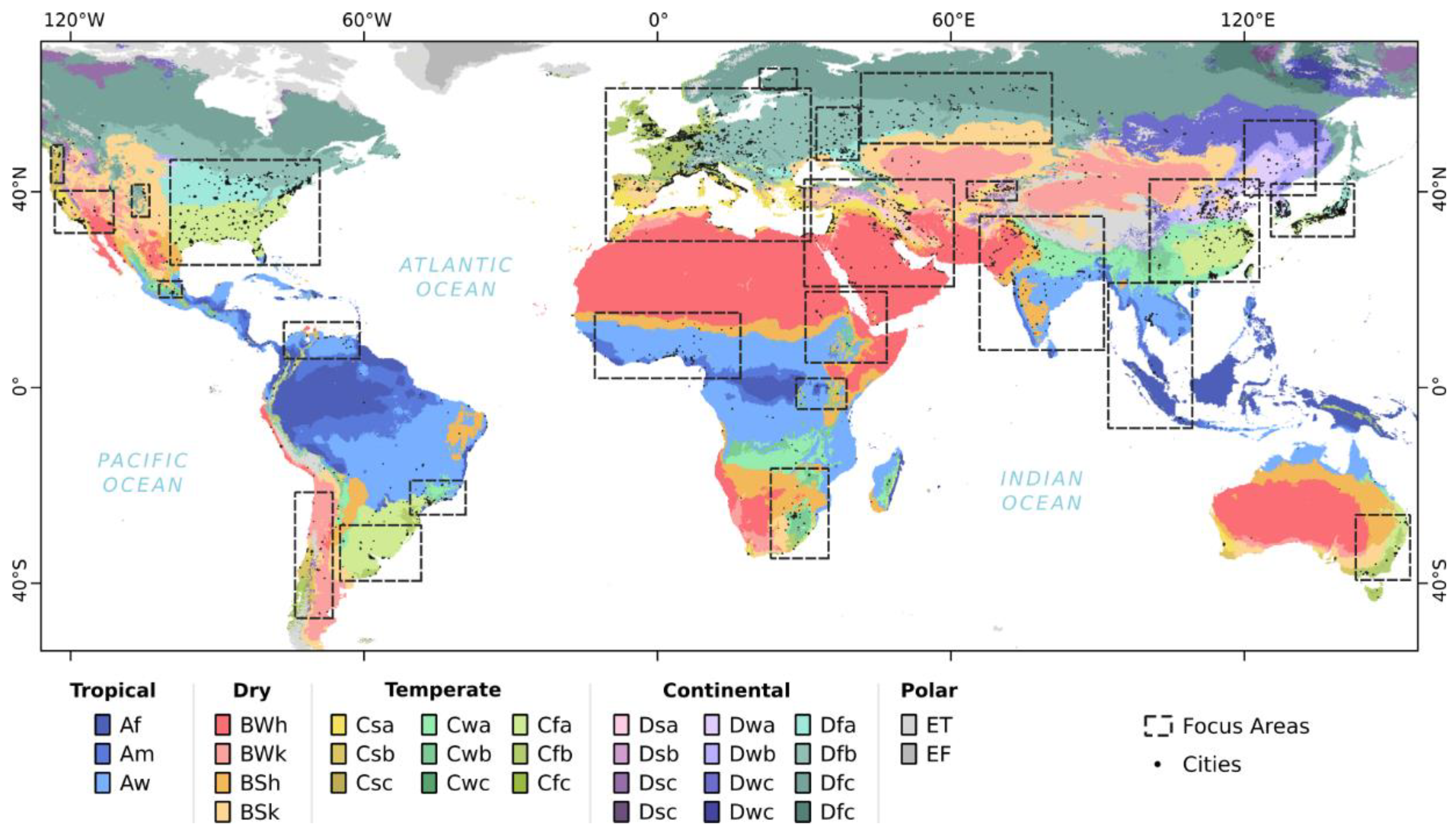
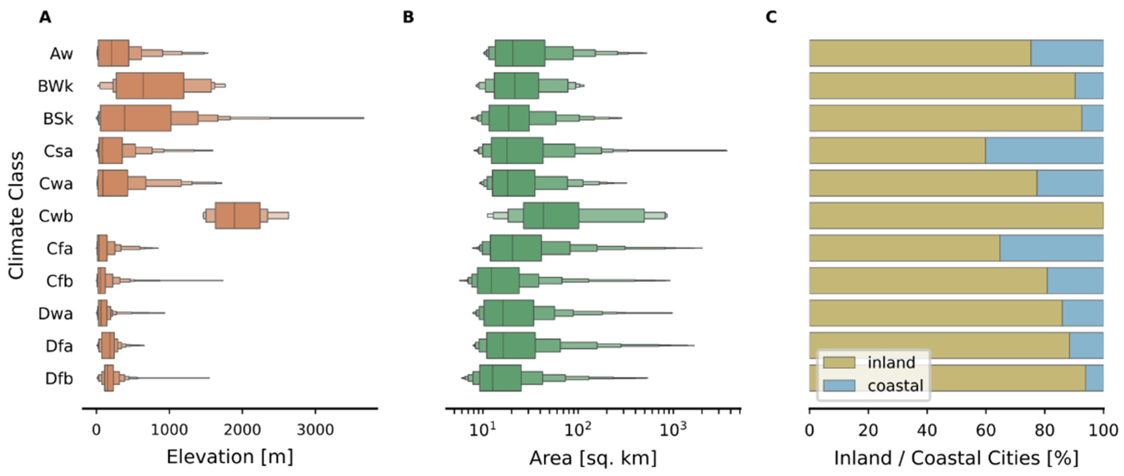
50], we delineate 1511 global cities in one tropical, two dry, five temperate, and three continental Köppen–Geiger classes (
Table 2). The location and the number of cities per class is presented in
Figure 2, while their characteristics (area, elevation, and percentage of coastal/inland cities) are discussed in
Appendix B. From these 11 classes, 10 include more than 50 cities, 6 more than 100 cities, and 1 more than 300 cities. The majority (90.5%) of them are located in Asia (40.0%), Europe (27.5%), and North America (23.0%), and only 9.5% are in Africa (5.9%), South America (2.7%), and Oceania (0.9%). In
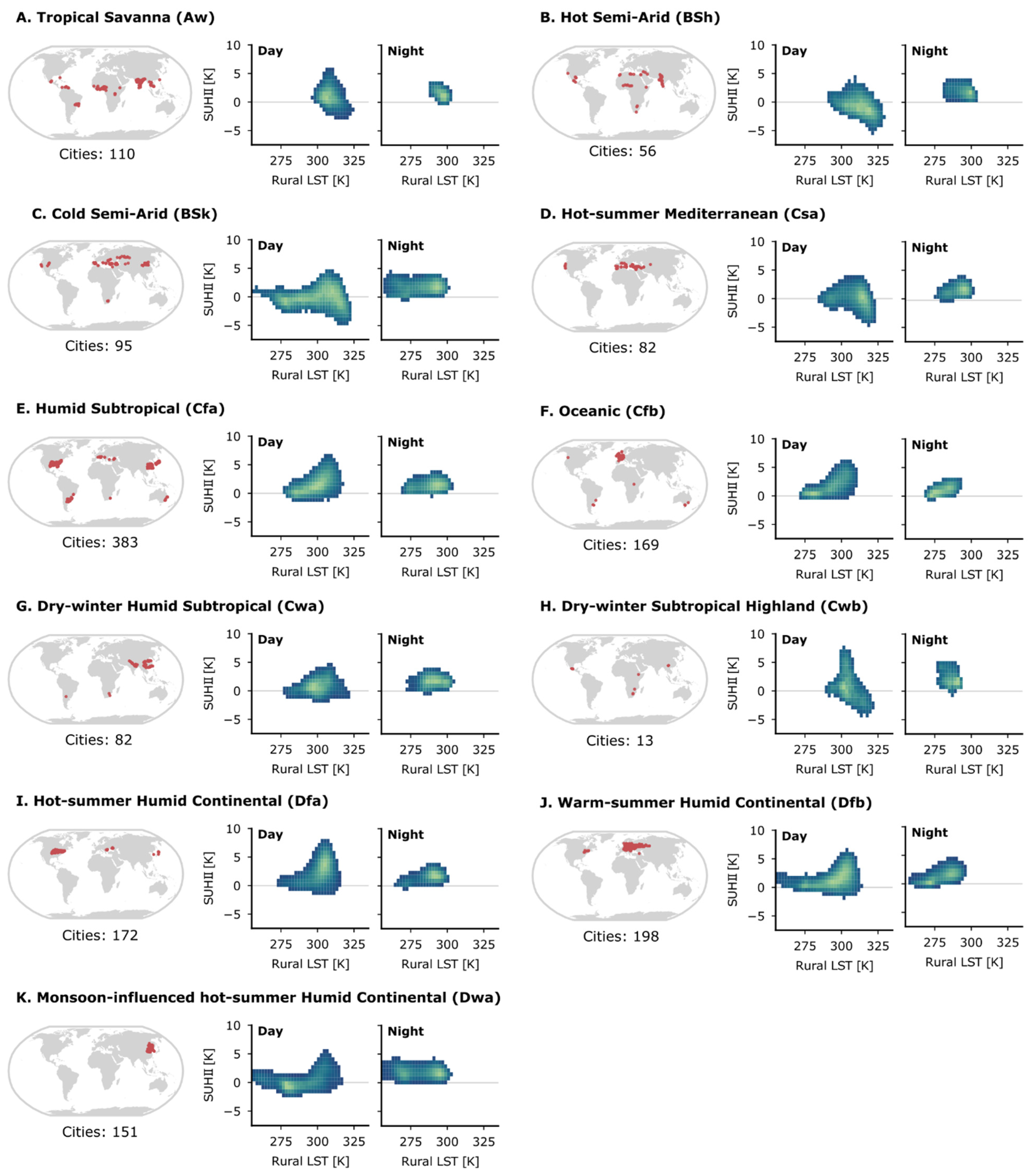
Figure 2, we also present the daytime (~10:30 local time) and nighttime (~22:30 local time) SUHII climatology of each class as the bivariate distribution of the daily SUHII and LST
rural that we have randomly sampled using the months as strata.
The tropical class is the Aw (tropical savanna), which comprises African, Asian, and South American cities (
Figure 2A). The Aw climate has two distinct seasons—a wet and a dry—and is warm throughout the year. This weak seasonality is evident in the SUHII climatologies in
Figure 2A, which are shaped like convex blobs. The interquartile range (shown as [Q
25, Q
75], where Q
25 and Q
75 are the first and third quartiles) of the Aw SUHII is [−0.4 K, 3.1 K] for the daytime and [0.5 K, 2.2 K] for the nighttime. The corresponding LST
rural values are [306 K, 315 K] and [293.7 K, 298.9 K], respectively, which make the Aw the climate with the least intra-annual variation in our analysis (the corresponding means are shown in
Table 3). The dry classes are the BSh (hot semi-arid) and the BSk (cold semi-arid). They are intermediate climates between desert and humid climates and are usually dominated by grasslands and shrubs. In our analysis, the BSh is represented mainly by cities in India, Africa, Mexico, and the Middle East, while the BSk is represented by cities in Europe and Asia. The shape of the BSh and BSk SUHII climatologies is more complex than that of the Aw and clearly influenced by seasons (
Figure 2B,C). The interquartile range of the daytime SUHII (and LST
rural) is [−2.0 K, 0.8 K] ([305.7 K, 319.8 K]) for the BSh and [−1.4 K, 1.2 K] ([283.7 K, 310.3 K]) for the BSk. The corresponding nighttime values are [1.1 K, 2.8 K] ([288.0, K 298.9 K]) and [1.0 K, 2.8 K] ([270.1 K, 290.6 K]), respectively. The key characteristic of these two dry climates is that daytime SUHIIs are mostly negative, especially when the LST
rural is maximum.
The five temperate classes are the Csa (hot-summer Mediterranean), Cfa (humid subtropical), Cfb (oceanic), Cwa (dry-winter humid subtropical), and Cwb (dry-winter humid highland). Temperate climates are generally defined as environments with moderate rainfall, sporadic droughts, mild-to-warm summers, and cool-to-cold winter. They occur in mid-latitude regions and have four seasons (winter, spring, summer, and autumn). The Csa exhibits wet winters and hot, dry summers and is water deficient during part of the growing season. This makes the daytime climatology of the Csa (
Figure 2D) to be considerably different than that of the other temperate climates. It has a concave-down shape with negative summertime SUHIIs and an interquartile range of [−1.1 K, 1.3 K] for the SUHII and [294.2 K, 313.1 K] for the LST
rural. In contrast, the shape of the Csa nighttime climatology is convex and always positive with an interquartile range of [0.9 K, 2.5 K] and [282.4 K, 293.8 K], respectively. The Cfa is represented by cities in North and South America, Europe, Australia, and Asia (
Figure 2E), while the Cfb is represented by cities in western Europe (
Figure 2F). Their daytime (and nighttime) climatologies exhibit almost identical concave-up shapes, with the SUHII and LST
rural peaking almost simultaneously. The daytime interquartile range of the SUHII (and LST
rural) is [0.3 K, 3.2 K] ([292.9 K, 309.1 K]) for the Cfa and [0.4 K, 3.0 K] ([282.0 K, 301.5 K]) for the Cfb. The corresponding nighttime values are [0.7 K, 2.2 K] ([279.6 K, 294.8 K]) and [0.4 K, 1.9 K] ([275.1 K, 285.9 K]). The last two temperate classes, namely the Cwa and Cwb, are represented mainly by cities in Asia and Central America, respectively. The Cwa is a monsoon-influenced climate with dry winters and hot summers, while the Cwb is a climate mainly found in tropical and subtropical highlands with cold, dry winters and rainy summers. They both exhibit a completely different daytime SUHII climatology than the other temperate climates. The shape of the Cwa climatology is presented in
Figure 2G, while that of the Cwb is in
Figure 2H. The interquartile range of the daytime SUHII (and LST
rural) is [−0.1 K, 2.5 K] ([298.0, 311.0]) for the Cwa and [−1.0 K, 3.4 K] ([301.1 K, 310.0 K]) for the Cwb. The corresponding nighttime values are [1.0 K, 2.5 K] ([286.2 K, 298.1 K]) and [1.1 K, 3.4 K] ([282.5 K, 290.1 K]), respectively.
The three continental Köppen–Geiger classes are the Dfa (hot-summer humid continental), Dfb (warm-summer humid continental), and Dwa (monsoon-influenced hot-summer humid continental). The Dfa is represented mainly by cities in North America (
Figure 2I), while the Dfb (
Figure 2J) and the Dwa (
Figure 2K) are represented by cities in Europe and Asia, respectively. Continental climates occur within large landmasses away from the moderating effect of oceans and are characterized by an extreme range of annual near-surface air temperatures. They exhibit four distinct seasons (winter, spring, summer, and autumn) with warm-to-hot summers and cold, snowy winters. The shapes of the Dfa, Dfb, and Dwa climatologies (
Figure 2I–K) are almost identical and quite similar to that of the Cfa and Cfb (
Figure 2E,F). When the LST
rural is below 300 K, the daytime SUHII of continental climates is rather constant and close to 1 K. Above 300 K, the SUHII increases considerably and peaks when the LST
rural is maximum. The shape of the corresponding nighttime climatologies are rather flat and featureless like all the other climates presented in
Figure 2. The interquartile range of the daytime SUHII is [0.3 K, 3.3 K] for the Dfa, [0.2 K, 2.7 K] for the Dfb, and [−0.5 K, 2.5 K] for the Dwa. The corresponding nighttime values are [0.5 K, 2.1 K], [0.4 K, 2.4 K], and [1.1 K, 2.8 K]. The extreme range of continental annual temperatures is evident in the interquartile range of the daytime LST
rural, which is [282.9 K, 304.8 K] for the Dfa, [275.2 K, 302.4 K] for the Dfb, and [282.5 K, 306.7 K] for the Dwa. The corresponding nighttime values are [271.5 K, 290.2 K], [268.9 K, 285.7 K], and [270.1 K, 292.3 K].
3.2. SUHII Seasonal Hysteresis
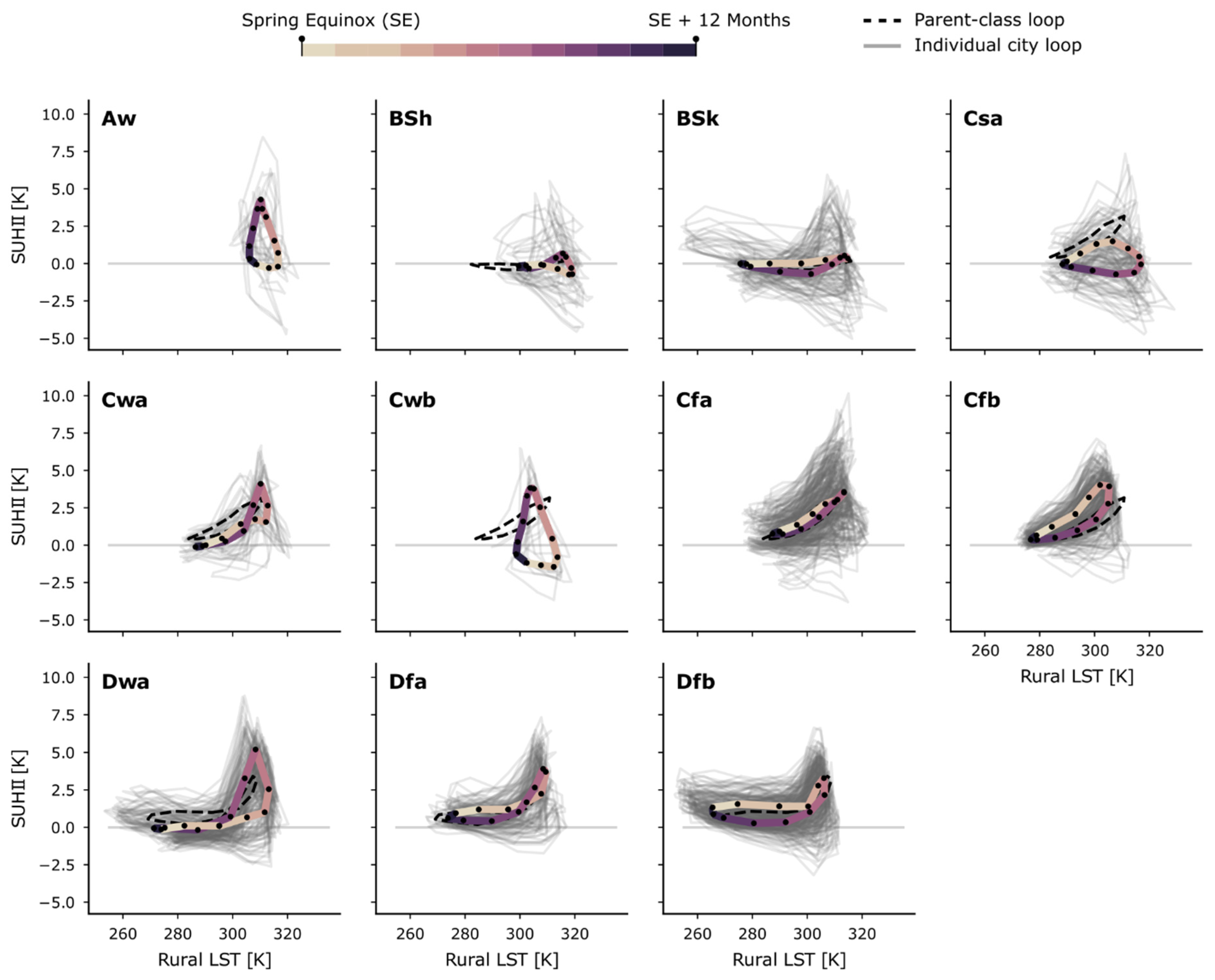
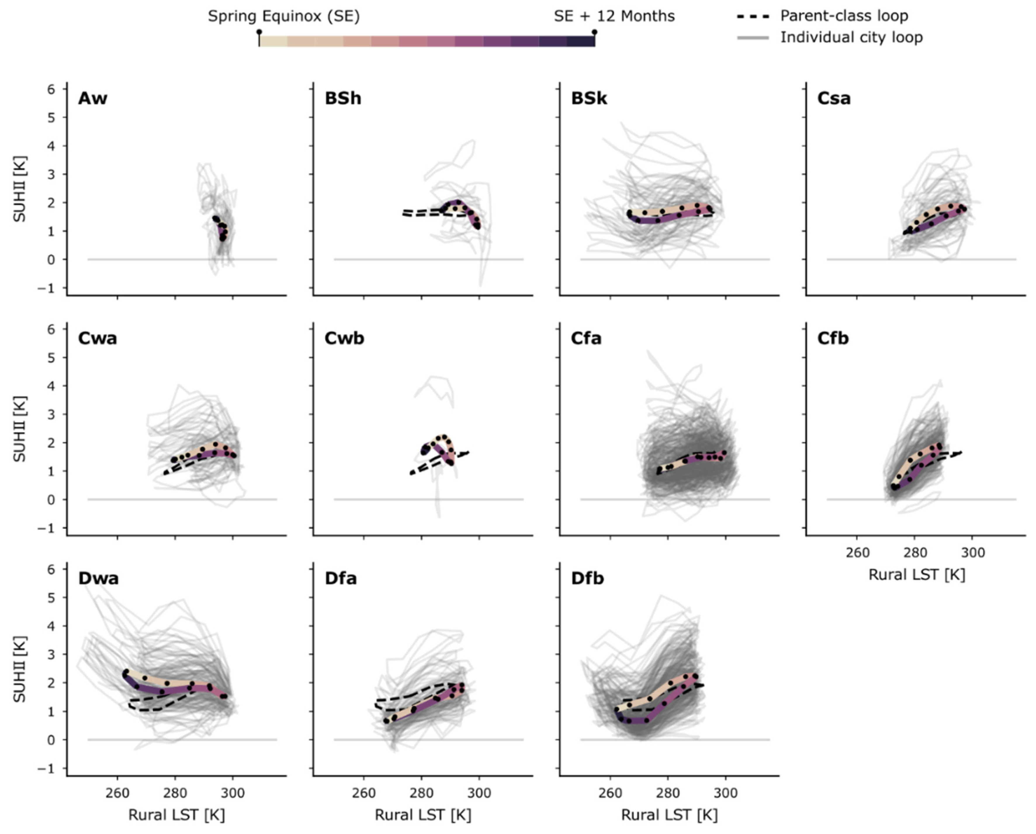
The daytime SUHII hysteresis loops of the examined climate classes are presented in
Figure 3. Overall, their shape matches well that of the SUHII climatologies and provides a clearer view of how the SUHII and LST
rural vary within the year. They are the most different for temperate climates (
Table 2), where each sub-class exhibits a distinct looping pattern. The daytime Cfa and Cfb hysteresis loops exhibit a concave-up pattern, as the model of Manoli et al. [
42] suggests, with the SUHII and LST
rural peaking almost simultaneously. The shape of the Csa loop exhibits a weak concave-down pattern, while that of the Cwa exhibits a twisted concave-up pattern. The shape of the Cwb daytime loop is convex (triangle-like), as is the case for the Aw. For cities in the Dfa, Dfb, and Dwa continental climates, the daytime SUHII hysteresis shows a concave-up pattern that is flat when the LST
rural is below ~300 K and peaks rapidly as the LST
rural increases. Similarly, to the Cfa and Cfb climates, the SUHII and LST
rural of the Dfa, Dfb, and Dwa become maximum almost simultaneously. For the BSh and BSk semi-arid climates, the daytime SUHII loops are rather flat. This result does not agree well with the shapes of the individual city loops shown in
Figure 3 (grey lines). Further investigations focusing on the BSh cities show that the shape of the individual hysteresis loops differs with geographic location and can take the form of concave-down, flat, twisted, and triangle-like loops (
Figure 4). These differences are attributed primarily to differences in the characteristics of the surrounding rural areas, which exert a strong influence on the SUHII [
24,
25], and suggest that semi-arid cities should be classified into even finer groups. Our analysis also shows that the shape of the humid temperate and continental loops is more stable than that of the dry-climate loops. This observation corroborates the remark of Manoli et al. [
42] that the shape of dry-climate loops is more susceptible to perturbations in the seasonality and the magnitude of rainfall. The direction of the daytime loops is clockwise in all cases, except for the Aw, BSh, Cwa, Cwb, and Dwa (
Figure 3).
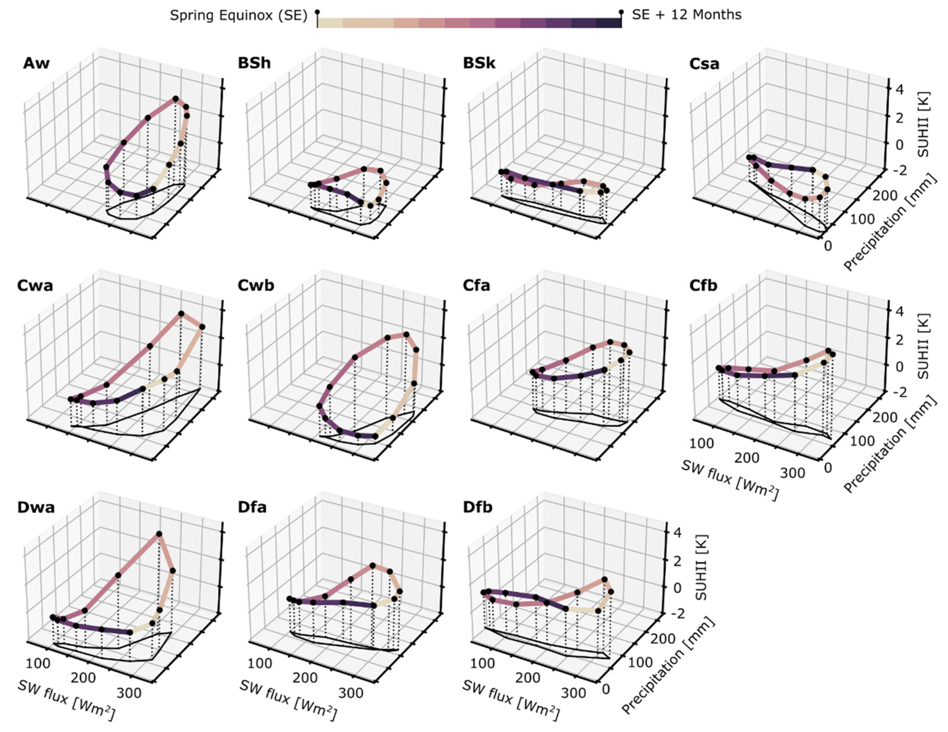
In
Figure 5, we present the seasonal variation of the daytime SUHII, SW, and precipitation for each Köppen–Geiger class examined in this work. We focus on these two variables because they have been shown to play a key role in the seasonality of the SUHII [
42]. For the Aw cities we observe that the SUHII peaks when the SW and precipitation are almost maximum. This is also the case for the Cwb cities in our analysis, which are located mainly in elevated regions within the tropics and the subtropics (
Figure 2H). In temperate and continental climates (Cfa, Cfb, Dfa, and Dfb), where the precipitation is rather constant throughout the year, the SUHII appears to vary mainly with the SW. This, however, is not the case for the Cwa and Dwa variates that exhibit a monsoonal tendency with a much higher precipitation in summer than in winter. In these climates, the SUHII intensifies as the summertime precipitation peaks, which suggests that monsoons influence the concave-up hysteresis of the SUHII in the Cwa and Dwa. The climate class with the most distinct behavior is the hot-summer Mediterranean (Csa), where the precipitation decreases as the SW increases. The anti-correlation between the SW and precipitation during spring and summer makes the Csa SUHII-SW-precipitation loop the only one with a clockwise direction (
Figure 5). The daytime SUHII of the Csa cities peaks in late spring/early summer and then starts to drop as the precipitation approaches its minimum and SW its maximum. During this phase, a significant portion of the natural vegetation begins to dry due to water stress [
54]. Under such water-limited conditions, the evapotranspiration of rural areas decreases, which impacts their ability to cool [
11,
42]. In dry-climate cities, the precipitation is low throughout the year and does not vary much with the SW (monsoon-influenced cities in India make the bulk of the examined BSh cities and are responsible for the precipitation peak in
Figure 5). The SUHII of the BSh and BSk cities does not vary with the SW either; however, as discussed above, this result is a fluke caused by averaging dissimilar SUHII loops (see
Figure 3 and
Figure 4). Overall,
Figure 5 shows that the SUHII of tropical, temperature, and continental cities is generally strongest when the SW and precipitation peak. Under these conditions, the vegetation surrounding each city reaches peak greenness, which in turn suggests that the observed SUHII increase should not be attributed solely to an increase in the urban LST.
The corresponding nighttime hysteresis loops are rather similar and exhibit mostly flat and concave-up patterns (
Figure 6). In humid temperate and continental climates, the SUHII increases and decreases almost in sync with the LST
rural, while in dry climates, the shape of the nighttime hysteresis loops is mainly flat. The looping direction is always clockwise and the classes with the most distinct nighttime loops are the BSh for the dry climates, the Cfb for the temperate, and the Dwa for the continental. Contrary to the daytime, the shape of the individual BSh and BSk nighttime hysteresis loops are more alike and better represented by the mean loop (
Figure 6). In respect to the seasonal variation of the precipitation and SW, the nighttime SUHII of the Csa, Cfa, Cfb, Dfa, and Dfb cities is strongest when the SW peaks (
Figure 7). In contrast, the nighttime SUHII of the Aw cities is weakest when the precipitation and SW peak.
In
Figure 3 and
Figure 6, we also include the SUHII hysteresis of the dry, temperate, and continental parent classes (dashed lines) that we derive using the individual loops from all the relevant cities. The results support our thesis that aggregating multi-city data without considering the biome of each city can result in temporal means that fail to reflect the actual SUHII characteristics and show that the shape of each parent-class loop is determined by the climate sub-class with the most cities. This is particularly the case for the Cfa and Cfb, where the daytime temperate parent-class loop reflects their shape and is not representative of the other temperate sub-classes (e.g., Csa or Cwb, as seen in
Figure 3).
3.3. Month of Minimum and Maximum SUHII
The month when the SUHII of each hysteresis loop is maximum and minimum in absolute values is shown with black dots in
Figure 8 and
Figure 9 (the corresponding magnitudes are provided in
Table 4). The colored dots refer to the individual city loops and indicate the variability in the examined cities. For the Aw cities, the daytime SUHII is strongest in September (4.3 ± 0.8 K) and weakest in February (−0.1 ± 0.7 K). The peak occurs four months later than that of the daytime LST
rural and one month later than that of the precipitation (
Figure 8). The nighttime SUHII peaks in January (1.4 ± 0.2 K) and is least in September (0.8 ± 0.2 K), whereas the Aw LST
rural is maximum in May and minimum in December/January.
The daytime SUHII and LST
rural of semi-arid cities is generally strongest in summer. The nighttime SUHII peaks in November (1.9 ± 0.2 K) for the BSh and in June (2.0 ± 0.2 K) for the BSk, while the LST
rural peaks in August. In hot-Mediterranean (Csa) cities, the daytime SUHII is warmest in May (1.5 ± 0.4 K) and the LST
rural in August. In contrast, the nighttime SUHII peaks in July (1.8 ± 0.2 K) when the precipitation is minimum and the LST
rural is almost maximum. The month when the Csa SUHII and LST
rural are weakest is January (
Figure 9). The Csa is the only temperate climate where the daytime SUHII peak occurs in spring and not in summer.
In wet temperate climates, the SUHII is strongest in summer. It peaks in August for the Cfa and in June/July for the Cfb. The corresponding SUHII magnitudes are 3.6 ± 0.3 K and 4.0 ± 0.2 K for the daytime and 1.7 ± 0.1 K and 1.9 ± 0.1 K for the nighttime (
Table 4). The LST
rural and SW also peak in summer, while the precipitation is relative constant throughout the year (this explains the pronounced dispersion of the Cfa and Cfb colored dots in
Figure 8 and
Figure 9). The SUHII is weakest in December/January for both climate classes, with the Cfa exhibiting a slightly greater magnitude (~0.9 K vs. 0.4 K). The daytime SUHII of the Cwa and Cwb cities is maximum in August/September and minimum in December. This is also the case for the precipitation, SW, and LST
rural. The maximum daytime SUHII is equal to 4.1 ± 0.5 K for the Cwa and 3.8 ± 1.3 K for the Cwb, while the corresponding minimums are 0.0 ± 0.2 K and 0.2 ± 0.6 K, respectively (
Table 4). The nighttime SUHII peaks earlier than the LST
rural (in April/May vs. July/August) and is equal to 1.9 ± 0.2 K for the Cwa and 2.2 ± 1.1 K for the Cwb.
In continental climates (Dfa, Dfb, and Dwa), the SUHII and LST
rural are warmest in July/August. The only exception is the Dwa where the nighttime SUHII peaks in February (
Figure 8). The precipitation also peaks in July, while the SW peaks in June. The maximum daytime SUHII is 3.9 ± 0.4 K for the Dfa, 3.3 ± 0.2 K for the Dfb, and 5.2 ± 0.3 K for the Dwa. The corresponding nighttime values are 1.9 ± 0.1 K, 2.2 ± 0.1 K, and 2.4 ± 0.2 K. The daytime SUHII minimums occur in November/December and the nighttime in January/December, except for the Dwa which occurs in August (
Figure 9). The corresponding values are ~0 K for the daytime and 0.7 ± 0.1 K (Dfa, Dfb) and 1.5 ± 0.1 K (Dwa) for the nighttime.
Figure 8 and
Figure 9 also show that the daytime and nighttime, minimum and maximum SUHII do not always occur in the same month. We attribute this to the different mechanisms that drive the SUHII during the day and night.


