Technical Note

Investigating the Magnetotelluric Responses in Electrical Anisotropic Media

1
Guangxi Beibu Gulf Marine Research Center, Guangxi Academy of Sciences, Nanning 530007, China
2
Hubei Subsurface Multi-Scale Imaging Key Laboratory, Institute of Geophysics and Geomatics, China University of Geosciences, Wuhan 430074, China
3
College of Earth Sciences, Guilin University of Technology, Guilin 541006, China
4
Key Laboratory of Environment Change and Resources Use in Beibu Gulf, Ministry of Education, Nanning Normal University, Nanning 530001, China
*
Author to whom correspondence should be addressed.
Remote Sens. 2022, 14(10), 2328; https://doi.org/10.3390/rs14102328
Submission received: 21 March 2022 / Revised: 6 May 2022 / Accepted: 9 May 2022 / Published: 11 May 2022

Abstract

:
When interpreting magnetotelluric (MT) data, because of the inherent anisotropy of the earth, considering electrical anisotropy is crucial. Accordingly, using the edge-based finite element method, we calculated the responses of MT data for electrical isotropic and anisotropic models, and subsequently used the anisotropy index and polar plot to depict MT responses. High values of the anisotropy index were mainly yielded at the boundary domains of anomalous bodies for isotropy cases because the conductive differences among isotropic anomalous bodies or among anomalous bodies and background earth can be regarded as macro-anisotropy. However, they only appeared across anomalous bodies in the anisotropy cases. The anisotropy index can directly differentiate isotropy from anisotropy but exhibits difficulty in reflecting the azimuth of the principal conductivities. For the isotropy cases, polar plots are approximately circular and become curves with a big ratio of the major axis to minor axis, such as an 8-shaped curve for the anisotropic earth. Furthermore, the polar plot can reveal the directions of principal conductivities. However, distorted by anomalous bodies, polar plots with a large ratio of the major axis to minor axis occur in isotropic domains around the anomalous bodies, which may lead to the misinterpretation of these domains as anisotropic earth. Therefore, combining the anisotropy index with a polar plot facilitates the identification of the electrical anisotropy.

1. Introduction

Electrical anisotropy indicates that the conductivity of the earth is directionally dependent, which is attributed to preferred directions of stratification, schistosity, sulfides, fractures, and fluids among other factors [1,2]. Electrical anisotropy is widely distributed in rock masses, such as gneisses and shale, and extensive evidence has shown the existence of electrical anisotropy [3,4]. Nevertheless, there are still no mature approaches to identifying the anisotropic effects of isotropic properties, such as the strike direction of anisotropy. Meanwhile, recognizing electrical anisotropy elucidates tectonic fabrics in the lithosphere, sub-lithospheric mantle, and dynamics of the plate-tectonic system [4]. Hence, interpreting the MT field data considering anisotropy is critical.
The abundance of research and applications associated with MT fields in anisotropic earth has undergone a rapid boom in recent decades, fuelled by novel numerical methodology, availability of new extensive data sets, and new developments in MT data acquisition instruments and computer science. Investigations of electrical anisotropy using MT involve various aspects, such as detecting the anisotropic effects of the crust and mantle, identifying whether the directional variance in the MT responses is induced by electrical anisotropy or large-scale geological structure, and probing dynamics of the plate-tectonic system [2,4,5,6]. Conductivity anisotropy can also aid in the estimation of the quality of observed data, such as distortion by galvanic effects of near-surface scatters, for inversion and geological interpretation [7,8].
In addition, MT numerical modeling schemes are useful for revealing electrical anisotropy; therefore, 1D stratified anisotropic model simulations were presented as infrastructure [9,10,11,12]. However, 1-D interpretation of MT solutions may only partly reflect the intricate surveyed structure; thus, 2-D and 3-D induction problems should be considered to give insight into the MT wave propagation mechanism in actual earth. Rayleigh modeling is a technique that is conducive to simulating structures with smooth irregularities; hence, it is suitable for modeling topographic distortion, as well as anisotropic effects on synclinal and anticlinal structures regarding 2-D and 3-D MT problems [13,14]. The finite difference (FD) method is another efficient and direct approach toward discretizing partial differential equations satisfied by MT conductivity anisotropy problems with regular grids [15,16]; however, problems can easily arise while handling the discretization of intricate geological structures, or curved boundaries when defining the boundary conditions. In addition, it is more difficult for the FD to process conductivity discontinuities. The finite volume (FV) method, also called the cell-centered difference scheme, has relative merit over FD because handling conductivity discontinuities is easy. Moreover, the FV is a natural choice for the partial differential equations (PDEs) of electromagnetic (EM) fields that accord with conservation laws. Therefore, certain previous studies took advantage of FV to analyze MT anisotropic responses [17]. Whereas, unlike the finite element (FE) method [18,19], the functions that approximate the solution when utilizing the FV cannot be easily made of higher order. As a powerful numerical modeling technique, FE is a remarkable method for simulating electromagnetic fields in anisotropic media [20,21,22,23]. As FE can easily perform a self-adaptive, goal-oriented mesh refinement algorithm, which makes a complicated investigative domain, such as a sloping seabed, topography undulating roughly ashore, and a misshapen interface between conductivity discrepant prisms and discretization convenient to implement; therefore, significant developments have been achieved with respect to the investigation of MT anisotropy issues using unstructured mesh FE [24,25,26]. In addition to numerical modeling, an analytical formula is another approach to calculating MT responses in anisotropic earth. Qin and Yang [27] proposed a quasi-static analytic approach to calculating MT responses in a 2-D model composed of two vertical stratifications with axial anisotropy overlying a good conductive basement.
Many authors have presented certain significant methods for recognizing the electrical anisotropy in the earth. Dimensionality analysis based on the rotational invariants of the MT tensor is an approach to identifying electrical anisotropy [1]. They utilized the WAL dimensionality criteria [28,29] to recognize anisotropic media from 2D isotropic media. Subsequently, Martí [3] provided a comprehensive review of electrical anisotropy analysis, such as the modeling of the electromagnetic fields in anisotropic earth, identifying anisotropy based on their responses, and taking advantage of anisotropic responses in the inversion and interpretation process. Another parameter based on the MT rotational invariants is anisotropy index [30]. Nevertheless, the anisotropy index was seldom used to investigate the responses of 3D structures. Using a polar plot is another way of identifying anisotropy, such as recognizing anisotropy from the topography effects [31]. A polar plot can be applied to show the surface azimuthal apparent resistivity distributions, which fixes a center observational station and calculates apparent resistivities as a function of azimuth. Several geophysical investigations involved the application of polar plots; for example, rotating a Wenner array on a fixed station to obtain an apparent resistivity ellipse aided in the analysis of the properties of a subsurface joint system, because of the major axis of the resistivity ellipse in accordance with the strike of the primary joint set [32]. In addition, the axes of the apparent resistivity ellipse presented by the azimuthal resistivity survey facilitated the investigation of the carbonate ground-water flow regimes and determined the strike direction fractures [33,34]. The use of polar plots contributed to the identification of anisotropic responses in a dipping anisotropic half-space seafloor [9]. Polar plots can also aid in the study of the fracture rock bulk anisotropy by azimuthal self-potential [35]. Yang and Qin [36] used ellipsoids, Mohr circles, and geometric forms to analyze the resources of the anisotropic earth. Their approach provides a powerful tool for quantitatively analyzing the characteristics of resources in anisotropic earth.
We also used polar plots to present the responses of both the isotropic and anisotropic models. However, the polar plots of the isotropic models also showed anisotropic responses. Therefore, further study of the polar plots combined with other parameters is necessary. This study considers the anisotropy index and polar plots simultaneously to identify the anisotropy.

2. Methods

The procedure of MT modeling using the edge-based finite element (FE) method has reached a fairly mature state [26,37,38]. We will not expound on more than what is needed here. Due to the low investigative frequency of the MT, the displacement currents are negligible. Moreover, under the passive source hypothesis, simplified Maxwell’s equations can be expressed using a time-dependence e i ω t as follows:
× E = i ω μ 0 H
× H = σ ^
where E and H are the electric and magnetic fields, respectively, ω is the angular frequency, μ 0 is the magnetic permeability of the free space, and σ ^ is the conductivity tensor that can be produced by a unit quaternion, direction cosines, and rotation vector, respectively, to represent the anisotropic earth. This study followed the study conducted by Yin [39] who used three principal conductivities and three Euler angles to present the conductivity tensor.
From Equations (1) and (2), we obtained
× v 1 · × F i ω L · F = 0
which represents a general MT governing equation, where,   F E , H , v μ 0 , σ ^ , and 𝓛 σ ^ , μ 0 . Here, we first solve the case of electric fields and compute the magnetic fields using Equation (1); thus, Equation (3) becomes
× × E k 2 E = 0
where, k 2 = i ω μ 0 σ ^ . Equation (4) is the governing equation of the electric field. Using the boundary conditions and weighted residuals method presented by Xu [40], we obtained boundary value problems and weighted residual expression of MT. By discretizing the modeling domain with brick cells and applying vector basis functions [41], we can obtain a system of equations
K E = 0
To reduce the CPU time and RAM consumption, we used the compressed sparse row (CSR) format [42] to store the upper triangular part of the large, sparse, and symmetrical FE coefficient matrix, K , and used the direct method solver PARDISO to solve Equation (5) to obtain the electric fields at the center of each edge after imposing the Dirichlet boundary condition. Subsequently, the magnetic components can be solved using Equation (1). Therefore, MT responses, such as impedance tensor, apparent resistivity, and phase, can be computed in accordance with previous studies [9,24]. Consequently, we can use the anisotropy index and polar plots calculated from the impedance tensor to discriminate anisotropic responses from isotropic responses.
In this study, looking from the plan view, the x-axis is positive upward, the y-axis to the right, and the z-axis positive downward. We obtained the following formula for the anisotropy index from the study conducted by Lilley [30]:
p r = 1 2 Z x x r Z y y r 2 + Z x y r + Z y x r 2 Z x x r Z y y r Z x y r Z y x r  
where the subscript r denotes the real part of the corresponding impedance
According to Yin [9] who used a polar plot to exhibit the principal anisotropy directions, we obtained the impedance in a polar plot after tensor rotation.
Z r φ = Z y x cos 2 φ Z x y sin 2 φ Z x x Z y y sin φ cos φ
Z φ r = Z x y cos 2 φ Z y x sin 2 φ Z x x Z y y sin φ cos φ
Consequently, the azimuth-based apparent resistivities ρ r φ a and ρ φ r a ; and phases ϕ r φ and ϕ φ r will be computed from Z r φ and Z φ r .

3. Synthetic Examples

Three synthetic models, including two 1-D layered anisotropic models, one with seawater, and a 2-D anisotropic model, were used to verify the validity of the algorithm presented in this study. Subsequently, we calculated and studied the MT responses for a 3-D isotropic and anisotropic mode.

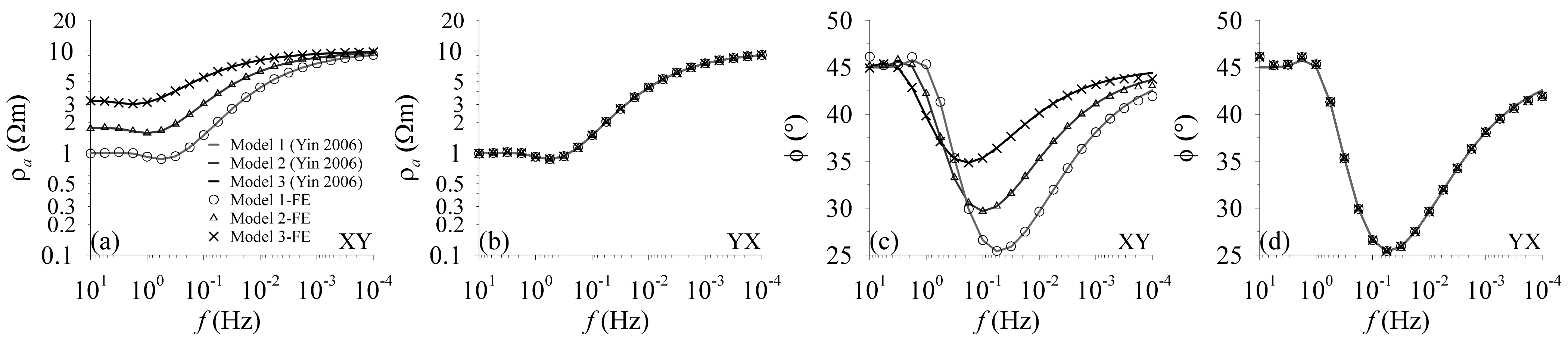
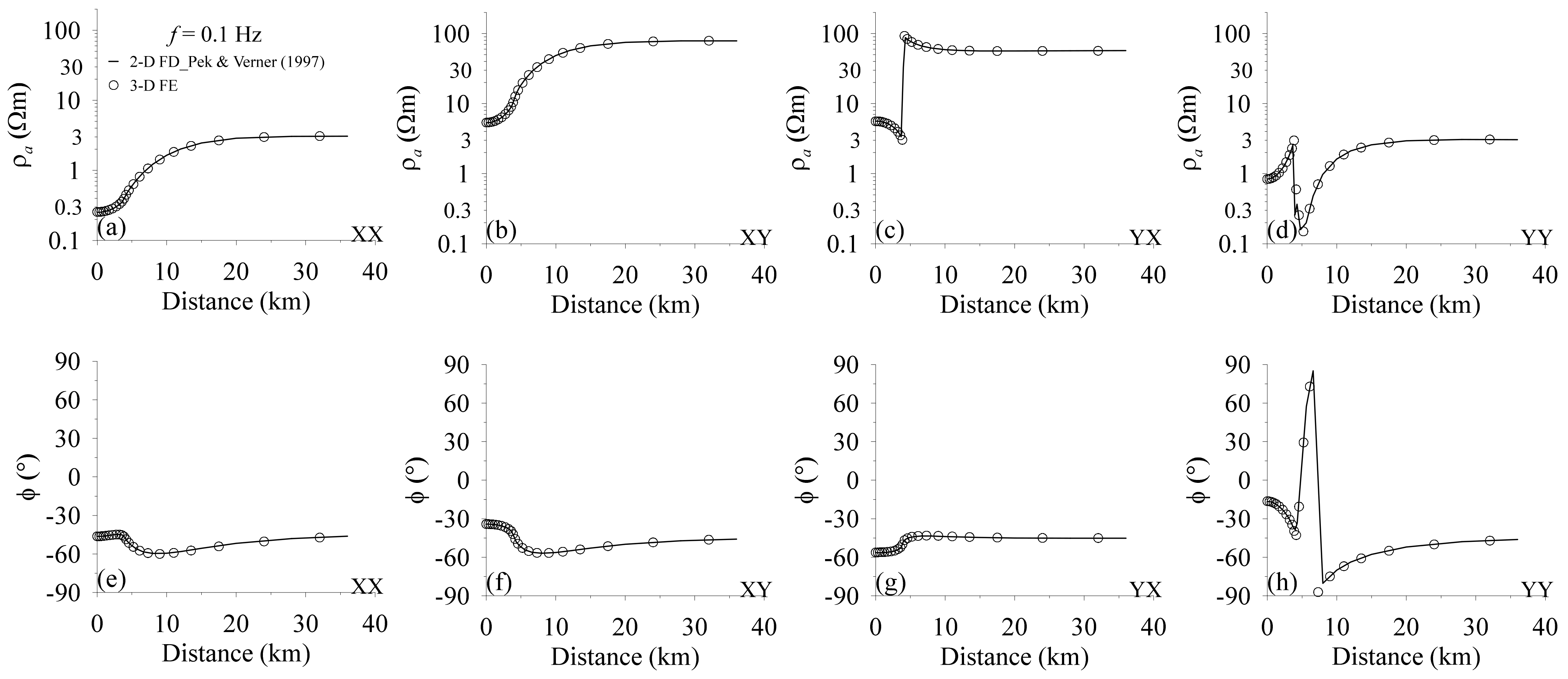
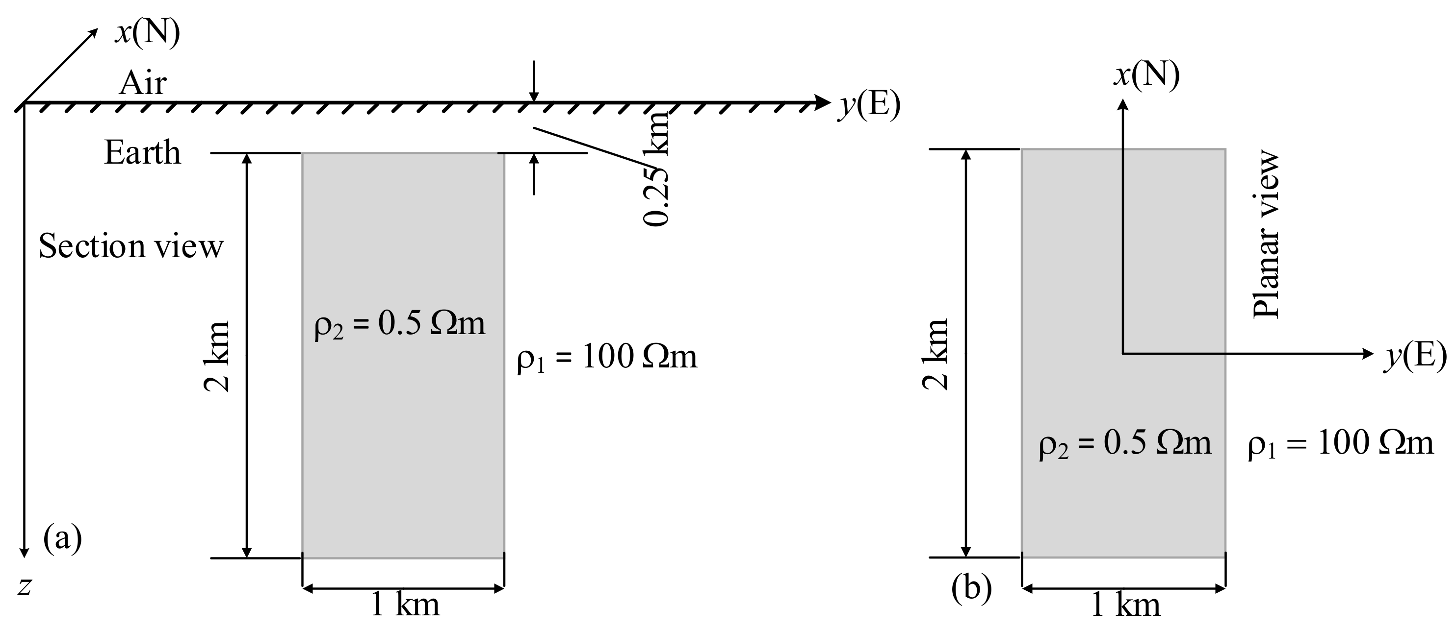
3.1. Verification Models

Above all, we calculated the MT responses of the GSLsz model [7] within the frequency range of 10−4 Hz < f < 320 Hz, with 43, 43, and 65 (including 7 layers in the air with a thickness of 144.11 km and a resistivity of 10 8   Ω m ) cells in the x-, y-, and z-directions, respectively, and compared the results with those of the 1-D anisotropic code reported by Pek and Santos [10], as shown in Figure 1. All apparent resistivity modes (XX, XY, YX, and YY) are quite consistent. The CPU time and peak memory consumptions are 95.64 s per frequency and 4.8 GB on a Lenovo ThinkPad P50 Mobile Workstation Laptop with Intel(R) Core(TM) i7-6700HQ CPU @2.60 GHz, 64 GB RAM. To further demonstrate the robustness of this approach, we tested our code on an anisotropic layered seafloor model [9]. The frequencies from 10−4 Hz to 10 Hz are divided into 21 logarithmically spaced frequencies. The cells number in x-, y-, and z-direction are 33, 33, and 64 (including 5 layers in the air with a thickness of 144 km and a resistivity of 10 8   Ω m , and 5 layers of seawater with a thickness of 1 km and a resistivity of 0.25   Ω m ). It took 38.63 s per frequency and cost 2.6 GB for the peak memory consumption. The apparent resistivities and phases in Figure 2 show great similarity and indicate the applicability of our code to marine MT modeling. Another test model was carried out using the 2-D electrical anisotropic model proposed by Reddy and Rankin [20], which was used for algorithm verification by Pek and Verner [15]. We discretized the model into 61, 61, and 47 (including 15 layers in the air with a thickness of 466.90 km and a resistivity of 10 8   Ω m ) cells in the x-, y-, and z-direction, respectively. It cost 190.96 s per frequency and 7.2 GB for the peak memory consumption. Figure 3 presents the modeling results obtained via the 2-D code of Pek and Verner [15] and our 3-D code, and they are practically identical.

3.2. Identification of Electrical Anisotropy

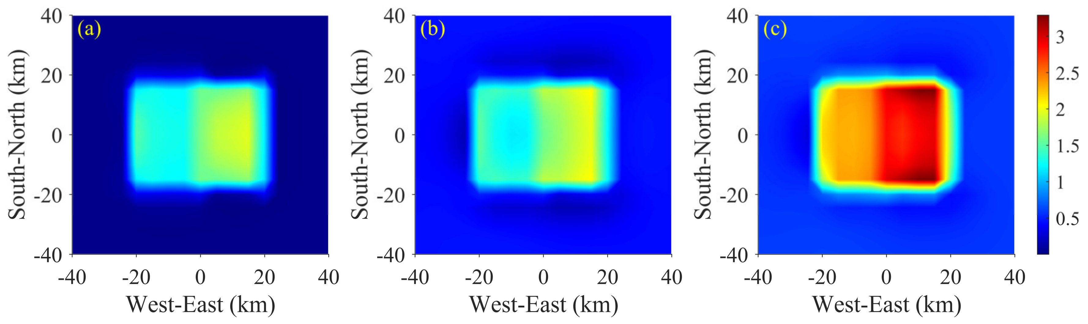
3.2.1. COMMEMI 3D-1A Model

The MT responses of the COMMEMI 3D-1A model (Figure 4) [43] for a frequency of 0.57 Hz were calculated and presented in terms of the anisotropy index and polar plot. Observed sites denoted by the ‘*’ symbol are distributed on the surface of the earth as shown in Figure 5. The anisotropy index and polar plot are shown at these sites. We used 70, 70, and 39 (including 10 layers in the air with a thickness of 10.56 km and a resistivity of 10 8   Ω m ) cells in x-, y-, and z-direction, respectively, to discretize the model. The CPU time and peak memory consumptions are 265.45 s per frequency and 7.8 GB, respectively. The anisotropy index for the isotropic case is shown in Figure 6a. The higher values of the anisotropy index mainly occur at the boundaries of the anomalous prism, because conductivity changes at the boundaries, and these domains can be treated as macro-anisotropy.
To investigate the responses of anisotropic earth, the embedded conductive isotropic prism of COMMEMI 3D-1A model is modified into an anisotropic prism with principal resistivity of ρ x x = 0.1   Ω m , ρ y y = 1000   Ω m , ρ z z = 10   Ω m , while the host rock maintains isotropy. The computational cost is approximate to the isotropic case. Compared to the isotropic case, the high values of the anisotropic indexes shown in Figure 6b are concentrated on the anomalous prism not only at the boundaries. Within the isotropic prism, the resistivity is homogeneous. Whereas, within the anisotropic prism, the resistivities are different in different directions. Therefore, the anisotropic index values are intense at the observation sites above the anisotropic prism, while they are weak for the isotropic case. The anisotropic indexes are relatively high at the boundaries for both isotropic and anisotropic cases, because the resistivity changes at the boundaries. It can be seen that the anisotropic indexes can show the positions where the resistivity is different.
As shown in Figure 7 and Figure 8, polar plots were used to investigate the electrical anisotropic responses of the COMMEMI 3D-1A model and the modified COMMEMI 3D-1A model. In the polar plot, the distances between the origin and each point on the curve represent the magnitude of the apparent resistivity, and the radial directions denote the directions of the observed horizontal electric or magnetic fields [9]. The red curve denoting ρ φ r a was computed using the azimuthal electric field and radial magnetic field. The blue curve denoting ρ r φ a was computed using the radial electric and azimuthal magnetic fields. They are always orthogonal. For the isotropic case (Figure 7), the polar plots of ρ r φ a and ρ φ r a at the outermost sites are approximately circles. When sites get closer to the anomalous prism, the ratios of the major axis to the minor axis of the graphics increase gradually for both ρ r φ a and ρ φ r a , especially at the boundaries of the anomalous prism. This can be interpreted as resistivity changes in the y-direction when approaching the west boundary of the anomalous prism. The resistivity ( 0.5   Ω m ) of the anomalous prism changes to resistivity of the background earth ( 100   Ω m ); hence, the major axis of ρ φ r a is in the y-direction. Analogously, the major axis of ρ φ r a is in the x-direction at the northern boundary. However, the ratios at sites above the anomalous prism become smaller, and the graphs become nearly circular.
For the anisotropic case (Figure 8), polar plots from the outermost sites to those above the anomalous prism show that the ratios grow gradually and become graphics such as an ‘8’ at the sites above the anomalous prism. As principal resistivity ρ x x = 0.1   Ω m and ρ y y = 1000   Ω m , the major axis of ρ φ r a is in the y-direction. The major axis denotes the largest principal value of the apparent resistivity tensor, and the minor axis denotes the smallest principal value.
The comparison of polar plots of isotropic (Figure 7) and anisotropic cases (Figure 8) shows that polar plots at the sites above the isotropic prism are approximately circles, while they have large ratios of the major and minor axes for the anisotropic case. As the resistivity within the isotropic prism is homogeneous, thus the polar curve is approximately a circle. Regarding the anisotropic prism, the resistivity is dependent on the direction, which gives rise to the curves with intense ratios of the major and minor axes. Since the major axis shows the high resistivity and the minor axis shows the low resistivity. However, distorted by the anomalous prism, polar plots at sites around the anomalous prism for both isotropy and anisotropy cases are rotated; that is, the major or minor axis of polar plots is not consistent with the original Cartesian coordinates. This phenomenon, that is, high ratios of the major and minor axes as well as the rotation of polar plots, may misrepresent the domains around the anomalous prism as anisotropic media.
The anisotropy index and polar plots show obvious differences between isotropy and anisotropy. High values of the anisotropy index are distributed at the boundary domains of the anomalous prism in the isotropic and anisotropic cases, and they occur across the anomalous domain in the case of anisotropy. Note that, although the anisotropy index values are high at the boundaries, the difference between the high and low index values in the isotropy case is smaller than in the anisotropy case. The anisotropy index directly reflects the intensity of the electrical anisotropy in the earth. In the polar plots, the major axis is approximately equal to the minor axis for the homogeneous media. For isotropy cases, large ratios occur at the domains ranging from the anomalous boundaries to a position that is approximately 0.75 to 1.5 times the length of the anomalous prism. The ratios for sites above the anomalous prism were also approximately equal to one. For anisotropy cases, the ratios for sites above the anomalous prism are the largest, and decrease gradually with sites extending to the isotropic host earth, and are approximately equal to one. These two parameters are useful for identifying anisotropy.
To investigate the general anisotropy, based on the aforementioned modified COMMEMI 3D-1A model, we rotated its principal conductivities around the axis using Euler rotation [39] and calculated the responses for 0.57 Hz. The computational cost is approximate to the isotropic case. For rotation around the x-axis by 30°, compared with the anisotropic model without rotation, the high values of the anisotropy index in Figure 9a are still distributed across the anomalous prism, yet it becomes x-axial asymmetric. The conductivity in the x-direction remains invariant when rotating around the x-axis, while conductivities in the y-z plane vary from principal conductivity in the y-direction to that in the z-direction. When rotated around the y-axis by 30°, it becomes asymmetric in the y-direction (see Figure 9b). For rotating around the z-axis by 30°, the conductivity in the z-direction is constant, and the conductivities in the x-y plane vary from the principal conductivity in the x-direction to that in the y-direction. The anisotropy index in Figure 9c also rotates by approximately 30° in the x-y plane. When rotating around the x-, y-, and z-axis by 30°, the high values shown in Figure 9d are easily recognizable, but anisotropy directions are not.
In polar plots, compared with the anisotropy case without rotation (Figure 8), the graphics shown in Figure 10 become x-axis asymmetric when rotating around the x-axis. More graphics with large ratios of the major axis to minor axis are distributed on the right side. For rotation around the y-axis, the graphics become y-axis asymmetric. More graphics in Figure 11 with large ratios of the major axis to minor axis are distributed at the top. The directions of the major and minor axes were consistent with those of the case without rotation. When rotating around the z-axis, the graphics at sites above the anomalous prism rotate evidently (Figure 12). The graphics at sites above and around the anomalous prism comprehensively are distorted. For rotation around the x-, y-, and z-axes, graphics at sites above the anomalous prism also rotate (Figure 13).
Using the anisotropy index, we identify the anisotropic prism within its boundaries, but cannot recognize the anisotropy direction. From the polar plot, the large ratio graphics appear at domains around the anomalous prism, but polar plots can provide anisotropy directions. Thus, combining these two parameters is significant for the accurate identification of the anisotropy.

3.2.2. COMMEMI 3D-2A Model

From the anisotropy index and polar plots of the COMMEMI 3D-1A mode or the modified COMMEMI 3D-1A mode, we found that the anomalous prism affected the surrounding domains. Therefore, it is necessary to investigate the responses of models composed of conjoined anomalous prisms. They may show the interaction between anomalous prisms. We used the COMMEMI 3D-2A model [43] (Figure 14) and modified COMMEMI 3D-2A model to calculate the responses of isotropic and anisotropic earth at frequencies of 0.1, 0.01, and 0.001 Hz. We used 88, 88, and 50 (including 15 layers in the air with a thickness of 83.64 km and a resistivity of 10 8   Ω m ) cells in x-, y-, and z-direction, respectively to discretize the model. The CPU time and peak memory consumptions are 823.75 s per frequency and 22.1 GB, respectively. The site locations are shown in Figure 15, the following anisotropy index and polar plots are presented at these sites. We changed the anomalous prisms numbered ① and ② into electrical anisotropy to obtain a modified COMMEMI 3D-2A model. The principal resistivity of anomalous prisms ① and ② are ρ 1 x x = 1   Ω m , ρ 1 y y = 500   Ω m , ρ 1 z z = 50   Ω m , ρ 2 x x = 0.5   Ω m , ρ 2 y y = 100   Ω m , and ρ 2 z z = 2000   Ω m . The computational cost is approximate to the isotropic case.
The anisotropy indexes of the COMMEMI 3D-2A model are shown in Figure 16. The high values for all frequencies occur at the boundaries of anomalous prisms. Meanwhile, some high values appear on anomalous prism ② for frequencies of 0.1 and 0.01 Hz. Based on the responses of the COMMEMI 3D-1A mode, these high values are caused by prism ①. The high values of the modified COMMEMI 3D-2A model in Figure 17 distribute at sites above anomalous prisms. Note that the interface between the anisotropic anomalous prisms can also be recognized.
As shown in Figure 18, similar to the COMMEMI 3D-1A model, polar plots with relatively large ratios of the major axis to the minor axis of the COMMEMI 3D-2A model for 0.1 Hz appear at sites at the boundaries of anomalous prisms. In accordance with the anisotropy index, the anisotropy reflected in the polar plots in Figure 18 is more obvious in anomalous prism ②. As shown in Figure 19, the anisotropic responses at the frequency of 0.01 Hz are similar to those at the frequency of 0.1 Hz in Figure 18, but more polar plots with a large ratio of the major axis to the minor axis extend to the isotropic host earth. For 0.001 Hz, the anisotropy in Figure 20 becomes more intense, which may result in incorrect anisotropy inference, but the anisotropy index shown in Figure 16c exhibits isotropy.
As for the anisotropy case, relatively large ratios of major axis to minor axis of polar plots are only yielded at sites above anomalous prisms at a frequency of 0.1 Hz (Figure 21). For frequencies of 0.01 Hz and 0.001 Hz, polar plots indicating anisotropy extend from the sites above anomalous prisms to the host earth, as shown in Figure 22 and Figure 23, because they are affected by the second anisotropic layer. A comparison of the anisotropy index and polar plot for the three frequencies shows that high values of the former focus on anomalous prisms, while the latter with a large ratio of the major axis to minor axis extends to the host earth gradually following a decrease in frequencies.

4. Conclusions

In this study, we investigated anisotropic characteristics, concentrating mainly on conductivity anisotropy, in 3-D MT responses using an edge-based finite element method. The conductivity tensor generated by the Euler rotation was used to describe the anisotropic earth. The boundary value problems of the electrical anisotropy case are analogous to those of isotropy, except that the scalar conductivity should be substituted by the conductivity tensor. Our results showed a great agreement with some published results. After verifying the algorithm, the MT responses of the anisotropic and isotropic models were calculated and compared in terms of anisotropy index and polar plots. The anisotropy index can directly identify isotropy and anisotropy; high values of the anisotropy index mainly appear at the boundary domains of isotropic anomalous prisms and across anisotropic anomalous prisms. However, it is difficult to confirm the rotation of the principal conductivity from the anisotropy index, while it is evident in polar plots. Polar plots show anisotropic responses at the domains around the anomalous prism, which may misrepresent these domains as anisotropic earth. Therefore, considering both the anisotropy index and polar plots simultaneously benefits us to identify the electrical anisotropy, namely, we can utilize the anisotropy index to recognize the anisotropy and define the boundaries of the anisotropic anomalous bodies. Meanwhile, we can employ a polar plot to identify the directions of the conductivity. Although this study is based on synthetic models, one can extend it to field data by using impedance calculated from two sets of orthogonal observed electromagnetic fields. However, the realistic subsurface electrical structures are more complicated than the synthetic models, and the investigations of anisotropic responses of field data require more attention in future studies.

Author Contributions

Conceptualization, T.L.; methodology, X.H. and L.C.; software, T.L. and G.X.; validation, X.H. and L.C.; formal analysis, X.H.; investigation, T.L. and G.X.; resources, X.H.; writing—original draft preparation, T.L.; writing—review and editing, X.H., L.C. and G.X.; visualization, T.L.; supervision, X.H., L.C. and and G.X.; funding acquisition, T.L., X.H., L.C. and G.X. All authors have read and agreed to the published version of the manuscript.

Funding

This research was funded by the National Natural Science Foundation of China, grant numbers 41630317, U1812402, 41904123, U20A20105, Natural Science Foundation of Guangxi Province, grant numbers 2018GXNSFBA138049, 2020GXNSFDA238021, Hubei Subsurface Multi-Scale Imaging Key Laboratory (China University of Geosciences), grant number SMIL-2019-04.

Data Availability Statement

The data associated with a part of the figures are uploaded to the repository figshare and available at the link https://figshare.com/articles/dataset/Investigating_the_magnetotelluric_responses_in_electrical_aniso-tropic_media/19682199 [44] after 29 April 2022.

Acknowledgments

The authors would like to appreciate Pek for his guidance on Euler’s rotation and electrical anisotropic theorem and for providing the 1-D and 2-D codes for validating the 3-D approach in this paper. We also thank Yin for providing the 1-D code of anisotropic marine MT modeling to help verify the applicability in marine MT of our 3-D code, as well as his constructive criticism of electrical anisotropic methodology about MT. In addition, we would also like to thank the anonymous reviewers and editors for their advantageous comments.

Conflicts of Interest

The authors declare no conflict of interest.

References

  1. Martí, A.; Queralt, P.; Ledo, J.; Farquharson, C. Dimensionality imprint of electrical anisotropy in magnetotelluric responses. Phys. Earth Planet. Inter. 2010, 182, 139–151. [Google Scholar] [CrossRef] [Green Version]
  2. Wannamaker, P.E. Anisotropy Versus Heterogeneity in Continental Solid Earth Electromagnetic Studies: Fundamental Response Characteristics and Implications for Physicochemical State. Surv. Geophys. 2005, 26, 733–765. [Google Scholar] [CrossRef]
  3. Martí, A. The Role of Electrical Anisotropy in Magnetotelluric Responses: From Modelling and Dimensionality Analysis to Inversion and Interpretation. Surv. Geophys. 2014, 35, 179–218. [Google Scholar] [CrossRef]
  4. Eaton, D.W.; Jones, A. Tectonic fabric of the subcontinental lithosphere: Evidence from seismic, magnetotelluric and mechanical anisotropy. Phys. Earth Planet. Inter. 2006, 158, 85–91. [Google Scholar] [CrossRef]
  5. Adetunji, A.Q.; Ferguson, I.J.; Jones, A.G. Reexamination of magnetotelluric responses and electrical anisotropy of the lithospheric mantle in the Grenville Province, Canada. J. Geophys. Res. Solid Earth 2015, 120, 1890–1908. [Google Scholar] [CrossRef]
  6. Jones, A.G. Electromagnetic interrogation of the anisotropic Earth: Looking into the Earth with polarized spectacles. Phys. Earth Planet. Inter. 2006, 158, 281–291. [Google Scholar] [CrossRef]
  7. Jones, A.G. Distortion decomposition of the magnetotelluric impedance tensors from a one-dimensional anisotropic Earth. Geophys. J. Int. 2012, 189, 268–284. [Google Scholar] [CrossRef]
  8. Heise, W.; Pous, J. Anomalous phases exceeding 90° in magnetotellurics: Anisotropic model studies and a field example. Geophys. J. Int. 2003, 155, 308–318. [Google Scholar] [CrossRef]
  9. Yin, C.C. MMT forward modeling for a layered earth with arbitrary anisotropy. Geophysics 2006, 71, G115–G128. [Google Scholar] [CrossRef]
  10. Pek, J.; Santos, F.A.M. Magnetotelluric impedances and parametric sensitivities for 1-D anisotropic layered media. Comput. Geosci. 2002, 28, 939–950. [Google Scholar] [CrossRef]
  11. Dekker, D.L.; Hastie, L.M. Magneto-telluric impedances of an anisotropic layered Earth model. Geophys. J. Int. 1980, 61, 11–20. [Google Scholar] [CrossRef] [Green Version]
  12. Okazaki, T.; Oshiman, N.; Yoshimura, R. Analytical investigations of the magnetotelluric directionality estimation in 1-D anisotropic layered media. Phys. Earth Planet. Inter. 2016, 260, 25–31. [Google Scholar] [CrossRef]
  13. Osella, A.M.; Martinelli, P. Magnetotelluric response of anisotropic 2-D structures. Geophys. J. Int. 1993, 115, 819–828. [Google Scholar] [CrossRef] [Green Version]
  14. Martinelli, P.; Osella, A. MT Forward Modeling of 3-D Anisotropic Electrical Conductivity Structures Using the Rayleigh-Fourier Method. J. Geomagn. Geoelectr. 1997, 49, 1499–1518. [Google Scholar] [CrossRef]
  15. Pek, J.; Verner, T. Finite-difference modelling of magnetotelluric fields in two-dimensional anisotropic media. Geophys. J. Int. 1997, 128, 505–521. [Google Scholar] [CrossRef]
  16. Hu, X.Y.; Huo, G.P.; Gao, R.; Wang, H.Y.; Huang, Y.F.; Zhang, Y.X.; Zuo, B.X.; Cai, J.C. The magnetotelluric anisotropic two-dimensional simulation and case analysis. Chin. J. Geophys.-Chin. Ed. 2013, 56, 4268–4277. [Google Scholar] [CrossRef]
  17. Han, B.; Li, Y.; Li, G. 3D forward modeling of magnetotelluric fields in general anisotropic media and its numerical implementation in Julia. Geophysics 2018, 83, F29–F40. [Google Scholar] [CrossRef]
  18. Castillo-Reyes, O.; de la Puente, J.; García-Castillo, L.E.; Cela, J.M. Parallel 3-D marine controlled-source electromagnetic modelling using high-order tetrahedral Nédélec elements. Geophys. J. Int. 2019, 219, 39–65. [Google Scholar] [CrossRef]
  19. Castillo-Reyes, O.; de la Puente, J.; Cela, J.M. PETGEM: A parallel code for 3D CSEM forward modeling using edge finite elements. Comput. Geosci. 2018, 119, 123–136. [Google Scholar] [CrossRef] [Green Version]
  20. Reddy, I.K.; Rankin, D. Magnetotelluric response of laterally inhomogeneous and anisotropic media. Geophysics 1975, 40, 1035–1045. [Google Scholar] [CrossRef]
  21. Xiao, T.; Liu, Y.; Wang, Y.; Fu, L.-Y. Three-dimensional magnetotelluric modeling in anisotropic media using edge-based finite element method. J. Appl. Geophys. 2018, 149, 1–9. [Google Scholar] [CrossRef]
  22. Cai, H.; Xiong, B.; Han, M.; Zhdanov, M. 3D controlled-source electromagnetic modeling in anisotropic medium using edge-based finite element method. Comput. Geosci. 2014, 73, 164–176. [Google Scholar] [CrossRef] [Green Version]
  23. Li, Y.; Dai, S. Finite element modelling of marine controlled-source electromagnetic responses in two-dimensional dipping anisotropic conductivity structures. Geophys. J. Int. 2011, 185, 622–636. [Google Scholar] [CrossRef] [Green Version]
  24. Li, Y. A finite-element algorithm for electromagnetic induction in two-dimensional anisotropic conductivity structures. Geophys. J. Int. 2002, 148, 389–401. [Google Scholar] [CrossRef] [Green Version]
  25. Key, K. MARE2DEM: A 2-D inversion code for controlled-source electromagnetic and magnetotelluric data. Geophys. J. Int. 2016, 207, 571–588. [Google Scholar] [CrossRef]
  26. Li, Y.; Pek, J. Adaptive finite element modelling of two-dimensional magnetotelluric fields in general anisotropic media. Geophys. J. Int. 2008, 175, 942–954. [Google Scholar] [CrossRef] [Green Version]
  27. Qin, L.; Yang, C. Analytic magnetotelluric responses to a two-segment model with axially anisotropic conductivity structures overlying a perfect conductor. Geophys. J. Int. 2016, 205, 1729–1739. [Google Scholar] [CrossRef]
  28. Weaver, J.T.; Agarwal, A.K.; Lilley, F.E.M. Characterization of the magnetotelluric tensor in terms of its invariants. Geophys. J. Int. 2000, 141, 321–336. [Google Scholar] [CrossRef] [Green Version]
  29. Martí, A.; Queralt, P.; Ledo, J. WALDIM: A code for the dimensionality analysis of magnetotelluric data using the rotational invariants of the magnetotelluric tensor. Comput. Geosci. 2009, 35, 2295–2303. [Google Scholar] [CrossRef]
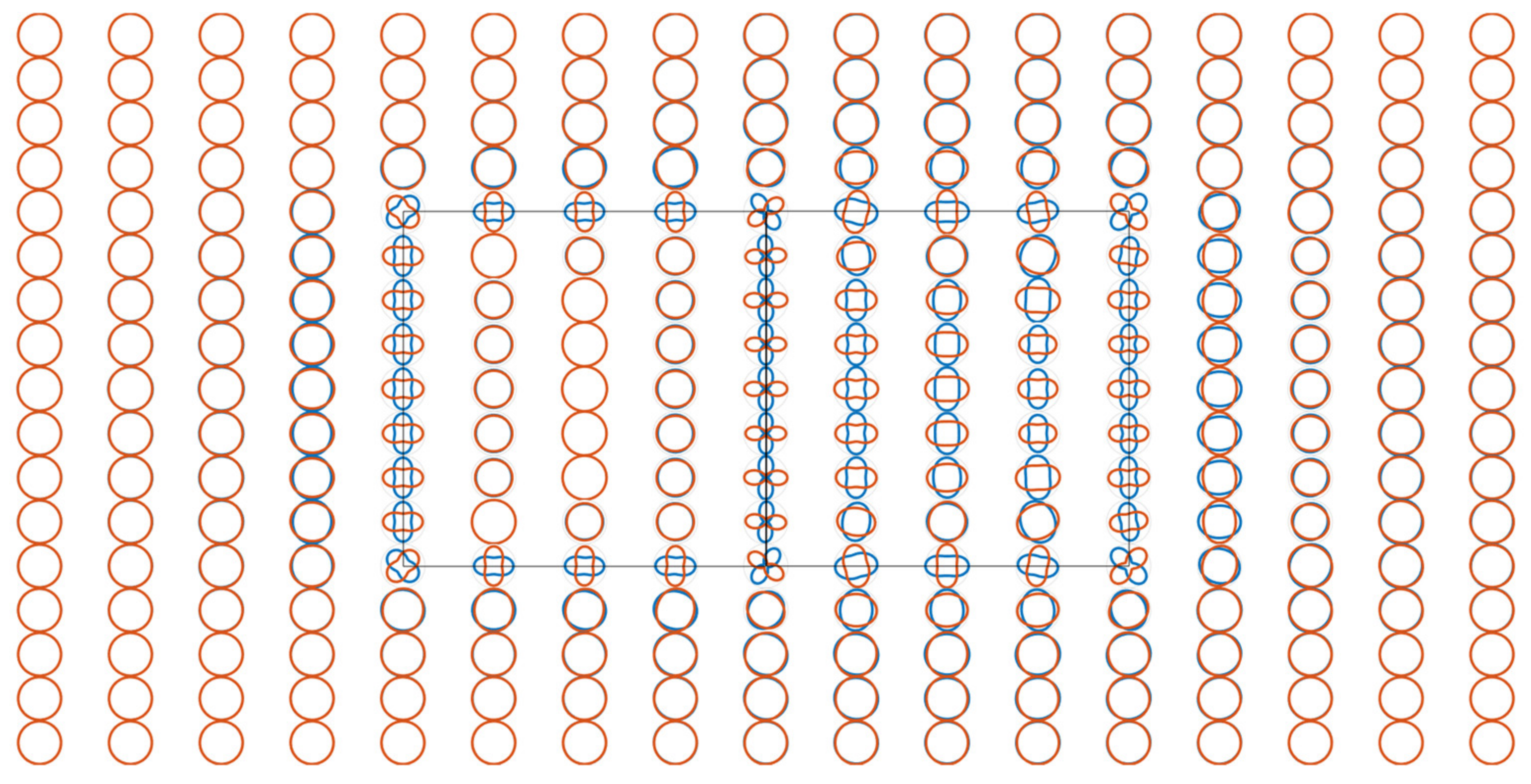
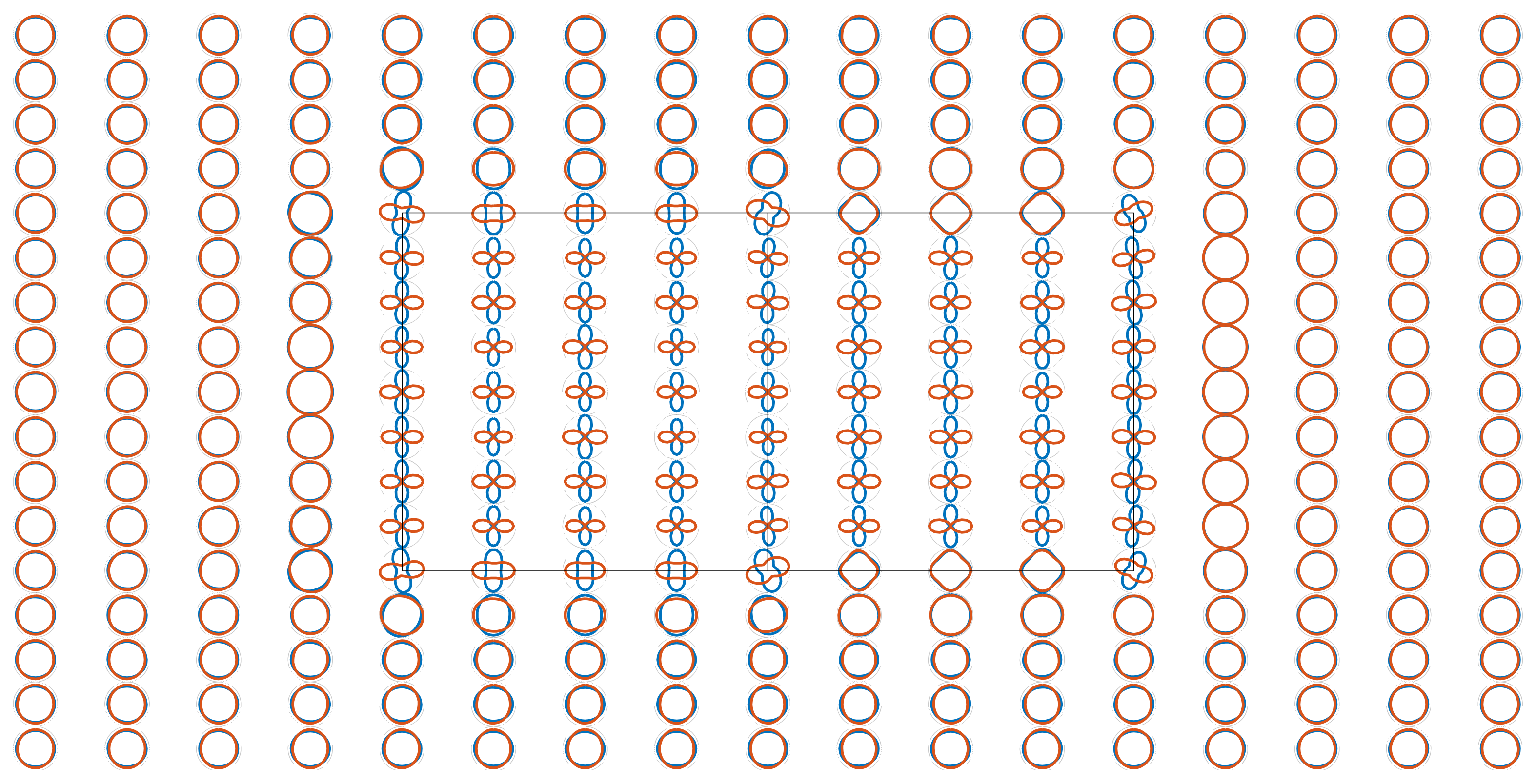
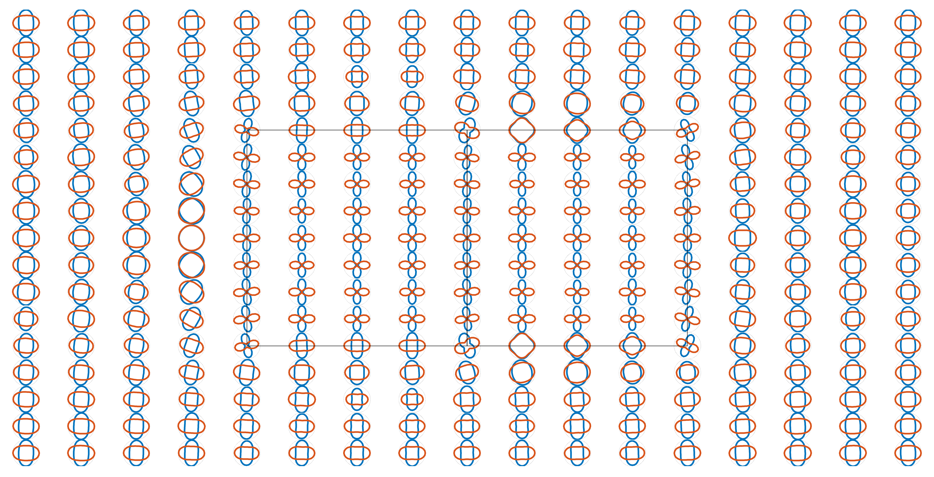
  30. Lilley, F.E.M. Magnetotelluric analysis using Mohr circles. Geophysics 1993, 58, 1498–1506. [Google Scholar] [CrossRef] [Green Version]
  31. Cao, X.Y.; Yin, C.C.; Zhang, B.; Huang, X.; Liu, Y.H.; Cai, J. A goal-oriented adaptive finite-element method for 3D MT anisotropic modeling with topography. Chin. J. Geophys.-Chin. Ed. 2018, 61, 2618–2628. [Google Scholar] [CrossRef]
  32. Taylor, R.W.; Fleming, A.H. Characterizing Jointed Systems by Azimuthal Resistivity Surveys. Groundwater 1988, 26, 464–474. [Google Scholar] [CrossRef]
  33. Ritzi, R.W.; Andolsek, R.H. Relation Between Anisotropic Transmissivity and Azimuthal Resistivity Surveys in Shallow, Fractured, Carbonate Flow Systems. Groundwater 1992, 30, 774–780. [Google Scholar] [CrossRef]
  34. Busby, J.P. The effectiveness of azimuthal apparent-resistivity measurements as a method for determining fracture strike orientations. Geophys. Prospect. 2000, 48, 677–695. [Google Scholar] [CrossRef]
  35. Wishart, D.N.; Slater, L.D.; Gates, A.E. Fracture anisotropy characterization in crystalline bedrock using field-scale azimuthal self potential gradient. J. Hydrol. 2008, 358, 35–45. [Google Scholar] [CrossRef]
  36. Yang, C.-f.; Qin, L.-j. Graphical Representation and Explanation of the Conductivity Tensor of Anisotropic Media. Surv. Geophys. 2020, 41, 249–281. [Google Scholar] [CrossRef]
  37. Farquharson, C.G.; Miensopust, M.P. Three-dimensional finite-element modelling of magnetotelluric data with a divergence correction. J. Appl. Geophys. 2011, 75, 699–710. [Google Scholar] [CrossRef]
  38. Rivera-Rios, A.M.; Zhou, B.; Heinson, G.; Krieger, L. Multi-order vector finite element modeling of 3D magnetotelluric data including complex geometry and anisotropy. Earth Planets Space 2019, 71, 92. [Google Scholar] [CrossRef] [Green Version]
  39. Yin, C.C. Geoelectrical inversion for a one-dimensional anisotropic model and inherent non-uniqueness. Geophys. J. Int. 2000, 140, 11–23. [Google Scholar] [CrossRef] [Green Version]
  40. Xu, S.Z. Finite Element Method in Geophysics, 1st ed.; Science Press: Beijing, China, 1994. [Google Scholar]
  41. Jin, J.-M. The Finite Element Method in Electromagnetics, 2nd ed.; John Wiley & Sons: New York, NY, USA, 2002. [Google Scholar]
  42. Saad, Y. Iterative Methods for Sparse Linear Systems, Second Edition, 2nd ed.; Society for Industrial and Applied Mathematics: Philadelphia, PA, USA, 2003; p. 528. [Google Scholar]
  43. Zhdanov, M.S.; Varentsov, I.M.; Weaver, J.T.; Golubev, N.G.; Krylov, V.A. Methods for modelling electromagnetic fields Results from COMMEMI—The international project on the comparison of modelling methods for electromagnetic induction. J. Appl. Geophys. 1997, 37, 133–271. [Google Scholar] [CrossRef]
  44. Luo, T.; Hu, X.; Chen, L.; Xu, G. Investigating the Magnetotelluric Responses in Electrical Anisotropic Media. 2022. Available online: https://figshare.com/articles/dataset/Investigating_the_magnetotelluric_responses_in_electrical_aniso-tropic_media/19682199 (accessed on 29 April 2022).
Figure 1. Apparent resistivities for the GSLsz model obtained via the 1-D anisotropic code of Pek and Santos [10] and our 3-D edge-based FE algorithm. The symbols on the left and right column of the legend denote their results and this study, respectively. Twenty-one frequencies were generated within the range of 10−4 Hz < f < 320 Hz in terms of logarithmic equivalent space.
Remotesensing 14 02328 g001
Figure 2. Comparison of apparent resistivities and phases. Solid lines denote the results of Yin [9] and the symbols are the results of this study with respect to models 1, 2, and 3. (a,b) are apparent resistivities, and (c,d) are phases corresponding to XY and YX modes, respectively.
Remotesensing 14 02328 g002
Figure 3. Comparison between our resistivities and phases with the 2-D FD results of Pek and Verner [15] using the laterally inhomogeneous and anisotropic dyke model of Reddy and Rankin [20]. The solid line denotes the results of Pek and Verner [15], and circles show the results of this study. The frequency is 0.1 Hz. (ad) are apparent resistivities, and (eh) are phases corresponding to XX, XY, YX, and YY modes, respectively.
Remotesensing 14 02328 g003
Figure 4. The COMMEMI 3D-1A model. (a) The section view, looking from negative to positive in the x-direction. (b) The planar view, looking from negative to positive in the z-direction.
Remotesensing 14 02328 g004
Figure 5. Plan view of COMMEMI 3D-1A model. The * symbols denote the observed sites. The rectangle is the projection of the anomalous prism on the earth’s surface.
Remotesensing 14 02328 g005
Figure 6. Anisotropy index for a frequency of 0.57 Hz. (a) The COMMEMI 3D-1A model. (b) The modified COMMEMI 3D-1A model.
Remotesensing 14 02328 g006
Figure 7. Polar plots of COMMEMI 3D-1A model for a frequency of 0.57 Hz. The distances between the origin of coordinates and points on the curve represent the magnitude of apparent resistivity, and the radial directions indicate the observed directions of polarized electric fields. The red apparent resistivity ( ρ φ r a ) curves defined by the azimuthal electric and radial magnetic fields are orthogonal to the blue apparent resistivities ( ρ r φ a ) curves defined by radial electric and azimuthal magnetic fields and appear as an anisotropy paradox [9]. The red and blue curves with respect to polar plots adhere to the same definition in this figure. All pairs of polar plots are located at sites shown in Figure 5. The 0° azimuth was at the top of the polar plots and rotated clockwise, axis and tick labels were omitted due to the dense layouts of polar plots. The rectangle is the projection of the anomalous prism on the earth’s surface, but it is not consistent with the original scale.
Remotesensing 14 02328 g007
Figure 8. Polar plots of modified COMMEMI 3D-1A model for a frequency of 0.57 Hz.
Remotesensing 14 02328 g008
Figure 9. Anisotropy index of modified COMMEMI 3D-1A model for a frequency of 0.57 Hz. (a) Principal conductivity rotation around the x-axis by 30°. (b) Principal conductivity rotation around the y-axis by 30°. (c) Principal conductivity rotation around the z-axis by 30°. (d) Principal conductivity rotation around x-, y-, and z-axis by 30°.
Remotesensing 14 02328 g009
Figure 10. Polar plots of modified COMMEMI 3D-1A model for a frequency of 0.57 Hz. Principal conductivity rotation around the x-axis by 30°.
Remotesensing 14 02328 g010
Figure 11. Polar plots of modified COMMEMI 3D-1A model for a frequency of 0.57 Hz. Principal conductivity rotation around the y-axis by 30°.
Remotesensing 14 02328 g011
Figure 12. Polar plots of modified COMMEMI 3D-1A model for a frequency of 0.57 Hz. Principal conductivity rotation around the z-axis by 30°.
Remotesensing 14 02328 g012
Figure 13. Polar plots of modified COMMEMI 3D-1A model for a frequency of 0.57 Hz. Principal conductivity rotation around the x-, y-, and z-axis by 30°.
Remotesensing 14 02328 g013
Figure 14. COMMEMI 3D-2A model. (a) The planar view, looking from negative to positive in the z-direction. (b) The section view, looking from negative to positive in the x-direction. The number from ①−④ denote the media with different resistivity.
Remotesensing 14 02328 g014
Figure 15. Observed sites distributed on the plan view of COMMEMI 3D-2A model. The * symbols denote the observed sites. The rectangles are the projection of anomalous prisms on the Earth’s surface.
Remotesensing 14 02328 g015
Figure 16. Anisotropy index of COMMEMI 3D-2A model. (a) 0.1 Hz. (b) 0.01 Hz. (c) 0.001 Hz.
Remotesensing 14 02328 g016
Figure 17. Anisotropy index of modified COMMEMI 3D-2A model. (a) 0.1 Hz. (b) 0.01 Hz. (c) 0.001 Hz.
Remotesensing 14 02328 g017
Figure 18. Polar plots of COMMEMI 3D-2A model for a frequency of 0.1 Hz.
Remotesensing 14 02328 g018
Figure 19. Polar plots of COMMEMI 3D-2A model for a frequency of 0.01 Hz.
Remotesensing 14 02328 g019
Figure 20. Polar plots of COMMEMI 3D-2A model for a frequency of 0.001 Hz.
Remotesensing 14 02328 g020
Figure 21. Polar plots of modified COMMEMI 3D-2A model for a frequency of 0.1 Hz.
Remotesensing 14 02328 g021
Figure 22. Polar plots of modified COMMEMI 3D-2A model for 0.01 Hz.
Remotesensing 14 02328 g022
Figure 23. Polar plots of modified COMMEMI 3D-2A model for a frequency of 0.001 Hz.
Remotesensing 14 02328 g023
Publisher’s Note: MDPI stays neutral with regard to jurisdictional claims in published maps and institutional affiliations.

