MIMO: A Unified Spatio-Temporal Model for Multi-Scale Sea Surface Temperature Prediction

Abstract

Sea surface temperature (SST) is a crucial factor that affects global climate and marine activities. Predicting SST at different temporal scales benefits various applications, from short-term SST prediction for weather forecasting to long-term SST prediction for analyzing El Niño–Southern Oscillation (ENSO). However, existing approaches for SST prediction train separate models for different temporal scales, which is inefficient and cannot take advantage of the correlations among the temperatures of different scales to improve the prediction performance. In this work, we propose a unified spatio-temporal model termed the Multi-In and Multi-Out (MIMO) model to predict SST at different scales. MIMO is an encoder–decoder model, where the encoder learns spatio-temporal features from the SST data of multiple scales, and fuses the learned features with a Cross Scale Fusion (CSF) operation. The decoder utilizes the learned features from the encoder to adaptively predict the SST of different scales. To our best knowledge, this is the first work to predict SST at different temporal scales simultaneously with a single model. According to the experimental evaluation on the Optimum Interpolation SST (OISST) dataset, MIMO achieves the state-of-the-art prediction performance.

1. Introduction

Sea surface temperature (SST) refers to the temperature of the water from 1 millimeter to 20 meters below the sea surface. The ocean covers about three-quarters of the Earth’s surface and greatly influences global climate [1] and human activities [2]. As one key factor of ocean environment, SST affects global climate when assimilating and releasing heat. For instance, global precipitation is influenced by ocean evaporation, which is highly dependent on SST [3]. The widely known El Niño–Southern Oscillation (ENSO) phenomenon is an irregular periodic variation of SST in the tropical eastern Pacific Ocean, and occurs every 3∼5 years [4]. Therefore, accurately predicting SST could benefit various applications, e.g., weather forecasting, global warming prevention and extreme climate tracking.

Most existing methods for SST prediction are either numerical models or data-driven models. Numerical models [5], e.g., General Circulation Model (GCM), Integrated Forecast System (IFS) and Global Forecast Systems (GFS), predict SST by using differential equations to describe the relations between SST and other oceanic factors (e.g., sea surface height and air temperature) according to the laws of physics. Numerical models are usually of high complexity due to the large number of parameters, thus resulting in high computation cost. Data-driven SST prediction models predict SST by discovering the hidden regularity and patterns in historical SST data, and can be further divided into three sub-categories, i.e., statistical models [6], shallow neural network models [7,8,9] and deep learning models [10,11,12]. In contrast to numerical models, data-driven models require less domain knowledge and usually can achieve better prediction performance.

The existing methods mentioned above all focus on single-scale SST prediction, e.g., predicting the SST of the next seven days, and predicting the monthly average SST in the next one year. However, single-scale SST prediction has some disadvantages. First, we have to train different models for predicting different scales of SST, which is inefficient and costs many computation resources. Second, single-scale SST prediction ignores the correlations among SST of different scales. In practice, SST has different scales of temporal regularity. For example, the short-term SST usually depends on the long-term trends and periodicity of SST. In this case, the correlations of different scales of SST could be used for improving SST prediction.

To overcome the disadvantages of existing SST prediction methods, we propose multi-scale SST prediction to predict daily, weekly and monthly SST simultaneously. To this end, we face some technical challenges. First, multi-scale SST prediction needs to learn the features that can capture the regularity of different temporal scales of SST. Second, it is nontrivial to exploit the correlations among SST data of different scales. Third, the prediction model should be able to adapt to different scales of SST prediction.

To address these challenges in multi-scale SST prediction, we propose a new spatio-temporal model, i.e., the Multi-In and Multi-Out (MIMO) model. Concretely, the MIMO model first learns the spatio-temporal features for different scales of SST with independent learning blocks. Then, the learned features are fused to obtain unified feature representation. Finally, the MIMO model adaptively predicts different scales of SST with different prediction components. This is the first work that achieves unified prediction for SST of different temporal scales. The proposed model can learn the spatio-temporal features of SST well and fully take advantage of the correlations among different scales of SST to enhance the prediction.

The main contributions of this work are highlighted as follows.

• We raise the multi-scale SST prediction problem and highlight its technical challenges.
• We propose the MIMO model that can predict SST at multiple scales simultaneously with a single model. MIMO learns different scales of temporal regularity in SST and can be adapted to the requirements of SST prediction at different scales.
• We conduct extensive experiments on real SST datasets to evaluate the proposed method, and the experimental results shows that MIMO outperforms existing SST prediction methods, including CNN, LeNet and ConvLSTM.

The remainder of this work is organized as follows. Section 2 reviews the related work on SST prediction and analyzes the disadvantages of existing methods. Section 3 formally defines the problem of multi-scale SST prediction, and Section 4 gives the technical details of the proposed MIMO model. Section 5 reports the experimental results. Finally, Section 6 concludes the work.

2. Background

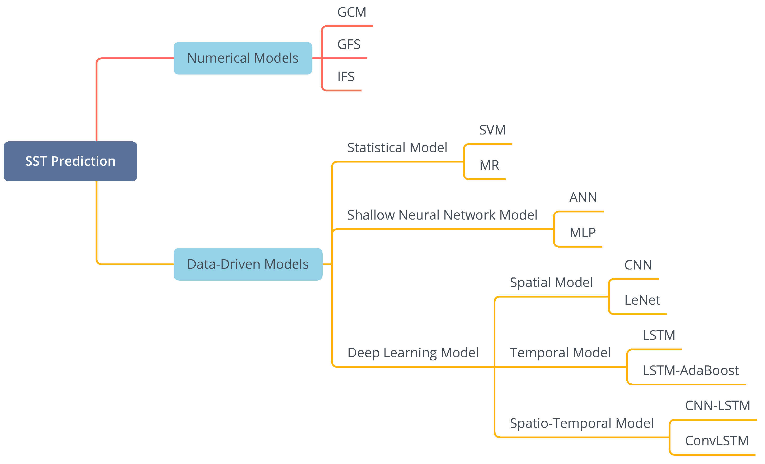
As discussed previously, existing SST prediction methods can be classified into numerical models and data-driven models, where data-driven models can be further divided into statistical models, shallow neural network models and deep learning models. Figure 1 shows the taxonomy of existing SST prediction methods and their representative models.

2.1. Numerical Models

Numerical models utilize mathematical equations to describe the underlying regularity in SST and its correlations with other oceanic and atmospheric variables [13,14,15]. This requires a better understanding of the dynamics of SST to design the prediction models. Representative numerical SST prediction models include General Circulation Model (GCM), Integrated Forecast System (IFS) and Global Forecast Systems (GFS).

GCM simulates the changes of the global climate by calculating the hourly evolution of the atmosphere based on the conservation laws for atmospheric mass, momentum, total energy and water vapor [16]. For example, Krishnamurti et al. used 13 coupled atmosphere-ocean models to predict SST [17].

The IFS model and GFS model are developed by the European Centre for Medium-Range Weather Forecasts (ECMWF) and the Command National Centers for Environmental Prediction (NCEP), respectively [18]. The IFS model can predict the SST of the following 10–15 days while the GFS model can predict the SST of the following 16 days. Both models contain multiple GCMs and can also predict other variables of the ocean and atmosphere.

Numerical models are usually of high computational complexity due to the large number of mathematical equations they have. In addition, numerical models are widely used for analyzing the global trends of SST but cannot predict the SST of high spatial resolutions well.

2.2. Data-Driven Models

Different from numerical models, data-driven models directly learn knowledge from historical SST data with machine learning techniques to conduct the prediction. Therefore, data-driven models depend more on SST data than the domain knowledge in ocean climate and environment.

2.2.1. Statistical Models

Statistical models for SST prediction learn the regularity and hidden patterns of SST from historical data [19,20]. Representative statistical models include support vector machine (SVM) and multi-linear regression (MR) model. SVM constructs a set of hyperplanes in a high dimensional space and uses these hyperplanes for classification and regression. For example, Lins et al. developed an SVM model that uses historical daily SST as input to predict the SST across the Northeastern Brazilian Coast [21] and the tropical Atlantic [6]. The MR model combines the SST anomaly index with the tropical Pacific SST anomaly to predict SST. It takes 12 months of historical SST data as the input and assumes that the SST follows some statistical assumptions. Then, the MR model uses a linearly weighted sum method to predict the SST of the following month [22]. Statistical models need feature engineering to extract features from SST data, which may result in the loss of some important information for SST prediction.

2.2.2. Shallow Neural Network Models

Shallow neural network (SNN) models are of high flexibility in fitting raw SST data [23,24,25]. Compared with the statistical models, SNN models can capture the nonlinear correlations in SST data, thus achieving better prediction performance. For instance, Patil et al. proposed an Artificial Neural Network (ANN) to predict the SST of the following 5 days [26]. Aparna et al. proposed an SNN that comprises three layers, i.e., input layer, linear layer and output layer, to predict the SST of the next day at specific locations [18]. Wei et al. separated SST time series data into monthly mean SST and monthly anomaly SST, and constructed two multilayer perceptron (MLP) models to generate the predicted results of SST [7].

Most shallow neural network models predict SST at some specific locations and ignore the spatial correlations and temporal regularity in SST. In addition, due to the limited learning ability, SNN models cannot fully exploit the large volume of historical SST data to train prediction models.

2.2.3. Deep Learning Models

With the substantial increase of SST data, statistical models and SNN models are unable to learn comprehensive knowledge from big SST data to further improve the prediction performance. Therefore, deep learning (DL) models have been introduced for SST prediction [27]. DL models can be classified into three sub-categories, i.e., deep spatial models, deep temporal models and deep spatio-temporal (ST) models.

Deep spatial models focus on learning the spatial correlations in SST data to achieve prediction. Ham et al. proposed a CNN-based model to predict the $Ni\tilde{n}o$ 3.4 index of the next 12 months based on the historical SST data of 12 months [28]. Zheng et al. proposed a model with stacked multiple CNN layers, Max Pooling layers and upsampling layers to predict the SST of the next day using the historical SST data of 14 days [11].

Deep temporal models focus on learning the temporal regularity in SST data to achieve prediction. Zhang et al. proposed an LSTM model to predict the SST in the next three days in the East China Sea with the historical SST data of 15 days [10]. Xiao et al. combined Ada-Boost and LSTM to predict the SST in the next 10 days in the East China Sea with the historical SST data of 40 days [29]. Yao et al. proposed an encoder–decoder model based on LSTM to predict the SST in the next 10 days using the historical data of 10 days [30].

Deep spatio-temporal models learn both spatial correlations and temporal regularity in SST to achieve prediction. Xiao et al. proposed a multi-layer convolutional LSTM model to predict the SST in the next 10 days with the historical SST data of 50 days in the East China Sea [12]. Weyn et al. combined the ConvLSTM model and the CNN model to predict the SST of the next three days with the historical SST data of 12 days [31]. Zhang et al. proposed a CNN-LSTM-based model to predict the SST in the next eight months using the historical SST data of 28 months [32]. In addition, deep graph models have also been used for SST prediction in recent years. Zhang et al. proposed a graph model MGCN that uses historical SST data of six days to predict the SST of the next three days. They used a temporal convolution to learn the temporal features of SST which are then put into the graph model to learn the spatial features [33].

In general, deep learning models can achieve better prediction performance than statistical models and shallow neural network models. However, all existing data-driven models only consider single-scale SST prediction, i.e., predicting daily or monthly SST separately, and cannot achieve multi-scale SST prediction.

3. Problem Definition

For SST prediction, we usually divide the target region of interest R into small grid regions of the same size along the latitude and longitude, and then predict the SST for each grid region. For example, as illustrated in Figure 2, the region $Ni\tilde{n}o$ 3.4 can be divided into 40 × 200 grid regions of size $0.{25}^{\circ }$ × $0.{25}^{\circ }$.

Assuming that the region of interest R is divided into c × d grid regions, the corresponding SST records at time slot t are denoted by $X_t\in {\mathbb{R}}^{c\times d}$. Data-driven SST prediction methods learn the underlying patterns of SST from historical SST data to predict the SST in the future. Specifically, the problem of single-scale SST prediction is defined as below.

Definition 1 (Single-Scale SST Prediction).

Given a sequence of historical SST records ${\mathbf{X}}_{t-a+1\to t}$$=($${\mathbf{X}}_{t-a+1}$, ${\mathbf{X}}_{t-a+2}$, …, ${\mathbf{X}}_t)$ of length a, single-scale SST prediction aims to predict the SST sequence ${\mathbf{X}}_{t+1\to t+b}$=(${\mathbf{X}}_{t+1}$, ${\mathbf{X}}_{t+2}$, …, ${\mathbf{X}}_{t+b})$ of length b in the future, i.e.,

$$\begin{array}{c}\hfill {\mathbf{X}}_{t+1\to t+b}=arg\underset{{\mathbf{X}}_{t+1\to t+b}}{max}p\left({\mathbf{X}}_{t+1\to t+b}\right|{\mathbf{X}}_{t-a+1\to t})\end{array}$$

(1)

In general, the time slot in single-scale SST prediction could be daily, weekly and monthly. For example, we can have the following SST prediction schemes:

• Using the historical daily SST of 10 days to predict the daily SST of the following seven days, where a = 10 and b = 7;
• Using the historical monthly SST of 36 months to predict the monthly SST of the following 12 months, where a = 36 and b = 12.

In existing studies on SST prediction, different scales of SST prediction are treated separately, i.e., training different prediction models for different scales of SST prediction. In this work, we aim to unify the prediction for multiple scales of SST and propose the problem of multi-scale SST prediction as defined below.

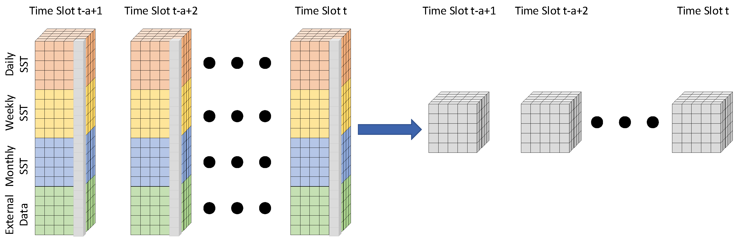
Definition 2 (Multi-scale SST prediction).

Given daily, weekly and monthly historical SST records ${\mathbf{X}}_{t-a+1\to t}^{daily}$, ${\mathbf{X}}_{t-a+1\to t}^{weekly}$ and ${\mathbf{X}}_{t-a+1\to t}^{monthly}$, respectively, multi-scale SST prediction aims to predict their corresponding records in the next b time slots, i.e.,

$$\begin{array}{c}\hfill \left\{{\mathbf{X}}_{t+1\to t+b}^{daily},{\mathbf{X}}_{t+1\to t+b}^{weekly},{\mathbf{X}}_{t+1\to t+b}^{monthly}\right\}=arg\underset{\left\{{\mathbf{X}}_{t+1\to t+b}^{daily},{\mathbf{X}}_{t+1\to t+b}^{weekly},{\mathbf{X}}_{t+1\to t+b}^{monthly}\right\}}{max}\\ \hfill p\left(\left\{{\mathbf{X}}_{t+1\to t+b}^{daily},{\mathbf{X}}_{t+1\to t+b}^{weekly},{\mathbf{X}}_{t+1\to t+b}^{monthly}\right\}\right|\left\{{\mathbf{X}}_{t-a+1\to t}^{daily},{\mathbf{X}}_{t-a+1\to t}^{weekly},{\mathbf{X}}_{t-a+1\to t}^{monthly}\right\})\end{array}$$

(2)

Figure 3 and Figure 4 illustrate the difference between single-scale SST prediction and multi-scale SST prediction. Single-scale SST prediction uses the same scale of historical SST data to predict the corresponding future SST records. Therefore, in single-scale SST prediction, the input has three dimensions, i.e., latitude, longitude and time slots. In contrast, multi-scale SST prediction considers multiple scales of historical SST data and achieves the prediction for all the scales of SST together, thus covering short-term, mid-term and long-term SST prediction. Therefore, in multi-scale SST prediction, the input has four dimensions, i.e., latitude, longitude, time slots and scales.

Considering that the prediction periods of most existing SST prediction methods are less than 12 time slots, we use the daily, weekly and monthly SST records of 36 time slots to predict the daily, weekly and monthly SST records in the next 12 time slots, i.e., $a=36$ and $b=12$. With such a setting, we can cover most of the prediction schemes in existing studies.

4. Methodology

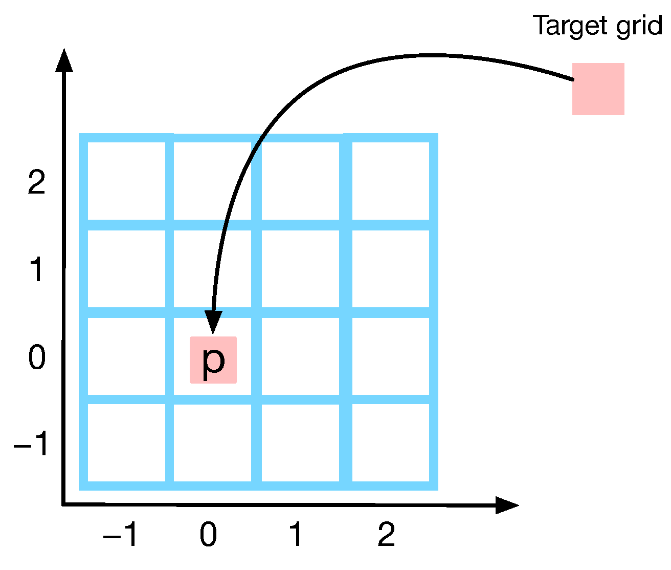
Figure 5 presents the overall architecture of the MIMO model which consists of an input layer, an encoder and a decoder. The input layer contains multi-scale SST data and some external factors, where external factors, including short wave radiation (SWR) and long wave radiation (LWR), are regarded as important influence factors for SST and are thus introduced to enrich the information for SST prediction. Considering that the spatial resolutions of SST data and external factors are usually different due to the difference in the ways of data collection, we use Bicubic Convolutional Interpolation (BCI) to align the spatial resolutions of external factors to that of SST data. The technical details of BCI are discussed in Appendix A.

In the encoder, MIMO uses five independent Zoom In Spatio-Temporal (ZIST) blocks to learn the hierarchical spatio-temporal features from multi-scale SST data and external factors and uses Cross Scale Fusion (CSF) to fuse the learned features. In the decoder, MIMO designs three independent components for monthly, weekly and daily SST prediction, respectively. Each component comprises three Zoom Out Spatio-Temporal (ZOST) blocks and one Full Connection (FC) layer, where ZOST blocks decode the fused features from the encoder stage and the FC layer achieves the final prediction.

4.1. Encoder

The encoder of the MIMO model has three spatio-temporal (ST) layers, and each ST layer consists of five Zoom In Spatio-Temporal (ZIST) blocks and one Cross Scale Fusion (CSF) sub-layer.

4.1.1. Zoom in Spatio-Temporal Block

Each ZIST block comprises Batch Normalization (BN), Dilated ConvLSTM (DCL), Rectified Linear Unit (ReLU) and Max Pooling (MP), where BN normalizes the data to avoid overfitting, DCL learns hierarchical features from the data using dilated convolution, ReLU filters the negative values to speed up the training process and MP reduces the number of model parameters and alleviates the position sensitivity.

Specifically, the DCL uses the dilated convolutional operation to replace the Hadamard product in LSTM to capture more spatial features. Figure 6 illustrates the 2D dilated convolutional operations that use intermittent connections between grids in traditional convolutional kernels. The dilation rate r is used to quantify the distance of intermittent connections between grids. Given a $k\times k$ convolutional kernel, the corresponding dilated kernel size is $k_d$ = $k+(k-1)(r-1)$. For example, in Figure 6, r = 1 corresponds to a normal convolution kernel, r = 2 corresponds to a dilated convolution kernel of size $k_d$ = 5, and r = 3 corresponds to a dilated convolution kernel of size $k_d$ = 7.

DCL will face the “gridding” issue [34] when multiple ST layers are stacked. To address this issue, MIMO sets different dilation rates r, i.e., 1, 2 and 3, for three ST layers, respectively.

In addition, the features learned by DCL can be affected by the changes of position, which makes the prediction model sensitive to specific positions and shapes. Meanwhile, with multiple stacked DCLs, we may lose the features for the marginal areas of feature maps. Both issues will damage the generalization of the MIMO model. We introduce Max Pooling (MP) to address these two issues. MP can reduce the model size and indirectly increase the receptive field of the kernel size to better learn spatial features in the data. In addition, MP brings the advantage of feature invariance to the prediction model, which avoids the learning errors due to location changes.

4.1.2. Cross Scale Fusion

MIMO learns the spatio-temporal features of different scales of SST and external features separately, and then fuses them together. Concretely, in each ST layer, the features learned from five ZISTs are fused with the CSF sub-layer. Each CSF sub-layer is a ConvLSTM layer with kernel size of $1\times 1$. As illustrated in Figure 7, CSF can reduce the dimensions of the outputs from five ZISTs to achieve the fusion.

4.2. Decoder

The decoder of the MIMO model comprises three independent components, each consisting of three Zoom Out Spatio-Temporal (ZOST) blocks and one Full Connection (FC) layer. As illustrated in Figure 5, each ZOST comprises BN, DCL, ReLU and Up Sampling (US) and can decode the fused features from the encoder to the target scale of SST.

We use the nearest neighbor upsampling method to decode the features from the encoder. The nearest upsampling method directly enlarges the fused features in proportion to the input data. As illustrated in Figure 8, the 2 × 2 feature map is converted to a 4 × 4 feature map using upsampling with 2 × 2 filters.

4.3. Loss Function

The objective of the MIMO model is to minimize the total error of the SST predictions of multiple scales, i.e.,

$$\begin{array}{c}\hfill Loss=\sum _{i=1}^3{\alpha }_i{L}_i({\mathbf{X}}_i^{obs},{\widehat{\mathbf{X}}}_i^{pre})\end{array}$$

(3)

where $L_i$ is the loss function for the i-th scale of SST, ${\alpha }_i$ is the weight parameter for loss function $L_i$, ${\mathbf{X}}_i^{obs}$ is the ground truth and ${\widehat{\mathbf{X}}}_i^{pre}$ is the predicted result of the MIMO model.

Since different scales of SST have different effects on the MIMO model, the loss functions corresponding to different scales of SST also have different effects on the total loss function. If we calculate the loss functions for SST predictions of different scales separately, the convergence speed of each loss function will be inconsistent. Hence, the MIMO model introduces weight parameters, i.e., ${\alpha }_i$, to balance the convergence speed between the loss functions for different scales of SST prediction. According to the experimental analysis, we set the weights for the loss functions of daily, weekly and monthly scales of SST prediction to $0.6$, $0.2$ and $0.2$, respectively.

The loss function $L_i$ for the i-th scale of SST is the mean squared error (MSE), calculated as below.

$$\begin{array}{c}\hfill L_i=\frac{1}{n}\sum {(X^{obs}-{\widehat{X}}^{pre})}^2\end{array}$$

(4)

where n is the number of samples. During the training, the model is optimized using Nadam [35].

5. Model Evaluation

We used the SST data from the El Niño region to compare the accuracy of our model to SVM, CNN, LeNet, LSTM and ConvLSTM. The time range of the SST dataset is from 1 January 1982 to 31 December 2019.

5.1. Datasets

We use the Optimum Interpolation SST (OI-SST) data from the National Oceanic and Atmospheric Administration (NOAA) and select the region of $Ni\tilde{n}o$ 3.4 as the target region for prediction. The NOAA $0.{25}^{\circ }$ OI-SST is a long-term climate data record that incorporates the observations from different platforms, e.g., satellites, ships, buoys and Argo floats, into a regular global grid format. The $Ni\tilde{n}o$ 3.4 region covers the area of [$5^{\circ }{00}^{\prime }$N∼$5^{\circ }{00}^{\prime }$S, ${120}^{\circ }{00}^{\prime }$W∼${170}^{\circ }{00}^{\prime }$W] and is divided into 40 × 200 grids of size $0.{25}^{\circ }$ × $0.{25}^{\circ }$. In addition, the data for the external factors SWR and LWR are from NCEP/NCAR Reanalysis 1.

The whole dataset is divided into three subsets for training, validation and testing, respectively. The ratio of the three subsets is 72:1. Concretely, the training dataset contains 8956 samples, the validation dataset has 2239 samples and the testing dataset has 1244 samples. In the experiments, we aim to predict the daily, weekly and monthly SST records in the next 12 time slots. The number of iterations for model training is set to 1000 and the training process could end early if the loss function no longer changes for 10 consecutive rounds. The experiments run on a 64-core Intel Xeon processor with 256 GB RAM and 3 NVIDIA RTX 2080Ti GPUs. All SST prediction models are implemented based on TensorFlow 1.15.0.

5.2. Evaluation Metrics

We use four evaluation metrics to measure the performance of SST prediction models. The equations of the four evaluation metrics are listed as follows.

$$\mathrm{MSE}=\frac{1}{n}\sum _i{(x_i-{\widehat{x}}_i)}^2,$$

(5)

$$\mathrm{RMSE}=\sqrt{\frac{1}{n}{\sum }_i{(x_i-{\widehat{x}}_i)}^2},$$

(6)

$$\mathrm{MAE}=\frac{1}{n}\sum _i|x_i-{\widehat{x}}_i|,$$

(7)

$$\mathrm{MAPE}=\frac{100\%}{n}\sum _i\left|\frac{x_i-{\widehat{x}}_i}{x_i}\right|.$$

(8)

where $\widehat{x}$ and x are the predicted value and the observed value, respectively, and n is the total number of predicted samples.

5.3. Results

5.3.1. Weight Evaluation

To decide the values for the weights ${\alpha }_i$ (i = $1,2,3$) in the loss function, we evaluate the performance of MIMO models with different settings as below, where $L_1$, $L_2$ and $L_3$ correspond to the loss functions of daily, weekly and monthly predictions, respectively.

• MIMO-122: $L_1=1$, $L_2=2$ and $L_3=3$.
• MIMO-911: $L_1=0.9$, $L_2=0.1$ and $L_3=0.1$.
• MIMO: $L_1=0.6$, $L_2=0.2$ and $L_3=0.2$.
• MIMO-433: $L_1=0.4$, $L_2=0.3$ and $L_3=0.3$.
• MIMO-244: $L_1=0.2$, $L_2=0.4$ and $L_3=0.4$.

Table 1. The results of MIMO with different settings for the weights of loss function.

Model	Daily				Weekly				Monthly				Total MSE
	MSE	RMSE	MAE	MAPE	MSE	RMSE	MAE	MAPE	MSE	RMSE	MAE	MAPE
MIMO-122	2.08	1.44	1.18	4.31%	1.88	1.37	1.11	4.07%	1.37	1.17	0.96	3.55%	1.99
MIMO-911	0.37	0.61	0.47	1.76%	0.61	0.78	0.60	2.22%	0.81	0.90	0.72	2.63%	0.44
MIMO	0.40	0.63	0.49	1.81%	0.50	0.71	0.55	2.04%	0.58	0.76	0.60	2.24%	0.45
MIMO-433	0.46	0.68	0.53	1.95%	0.58	0.76	0.60	2.20%	0.66	0.82	0.64	2.37%	0.56
MIMO-244	2.14	1.46	1.19	4.34%	2.01	1.42	1.14	4.19%	1.41	1.19	0.97	3.59%	1.80

presents the results of these models, where the best results are highlighted by boldface. As suggested by the table, MIMO-911 and MIMO achieve comparable performance and outperform all the other prediction models. Considering that MIMO has the best performance in predicting weekly and monthly SST and also achieves a high accuracy in predicting daily SST, we thus set $L_1=0.6$, $L_2=0.2$ and $L_3=0.2$ in the following experiments.

5.3.2. Model Comparison

To verify the effectiveness of the MIMO model, we compare it with five representative forecasting models: CNN, ConvLSTM, LeNet, LSTM and SVM. The experimental results are shown in

Table 2. The results of different SST prediction models.

Model	Daily				Weekly				Monthly				Total MSE
	MSE	RMSE	MAE	MAPE	MSE	RMSE	MAE	MAPE	MSE	RMSE	MAE	MAPE
MIMO	0.40	0.63	0.49	1.81%	0.50	0.71	0.55	2.04%	0.58	0.76	0.60	2.24%	0.45
ConvLSTM	2.78	1.67	1.36	5.01%	2.86	1.69	1.40	5.11%	2.53	1.59	1.33	4.80%	2.75
LeNet	0.41	0.64	0.47	1.77%	0.99	0.99	0.76	2.86%	1.52	1.23	0.95	3.59%	0.58
CNN	1.20	1.10	0.84	3.09%	1.73	1.32	1.05	3.88%	2.82	1.68	1.35	5.09%	1.42
LSTM	2.04	1.41	1.15	4.24%	1.88	1.35	1.10	4.01%	1.39	1.16	0.95	3.53%	1.88
SVM	0.43	0.64	0.48	1.77%	0.82	0.90	0.71	2.62%	1.13	0.96	0.85	3.18%	0.61
LeNet with EXT	0.56	0.75	0.56	2.09%	1.62	1.27	1.00	3.69%	1.54	1.24	0.99	3.75%	0.97
LSTM with EXT	1.86	1.34	1.10	4.04%	1.80	1.32	1.08	3.98%	1.36	1.15	0.94	3.49%	1.75
SVM with EXT	1.33	1.14	0.91	3.35%	1.21	1.09	0.86	3.13%	1.04	1.01	0.82	3.00%	1.25

, where the best results are highlighted by boldface. The MIMO model has the best total MSE. LeNet and SVM also achieve good prediction performance and largely outperform CNN, ConvLSTM and LSTM. Concretely, the MIMO model has the best performance in predicting weekly and monthly SST. MIMO also achieves comparable performance with LeNet in predicting daily SST on MAE and MAPE. The MIMO model is designed for multi-scale SST prediction and needs to balance the prediction performance of different scales. Therefore, the MIMO model can achieve accurate predictions for all three scales of SST.

In addition, we add more experiments to evaluate the influence of external factors, i.e., short wave radiation (SWR) and long wave radiation (LWR). In accordance with Table 2, after including the external factors, the performance of LSTM has a small increase while the performance of LeNet and SVM decreases. This is because some models cannot handle external factors well and the contribution of these external factors is also limited. In addition, our MIMO model still outperforms these models with external factors, which indicates that the MIMO model can fully take advantage of the correlations among SSTs of different scales to improve the prediction.

5.3.3. Visualization

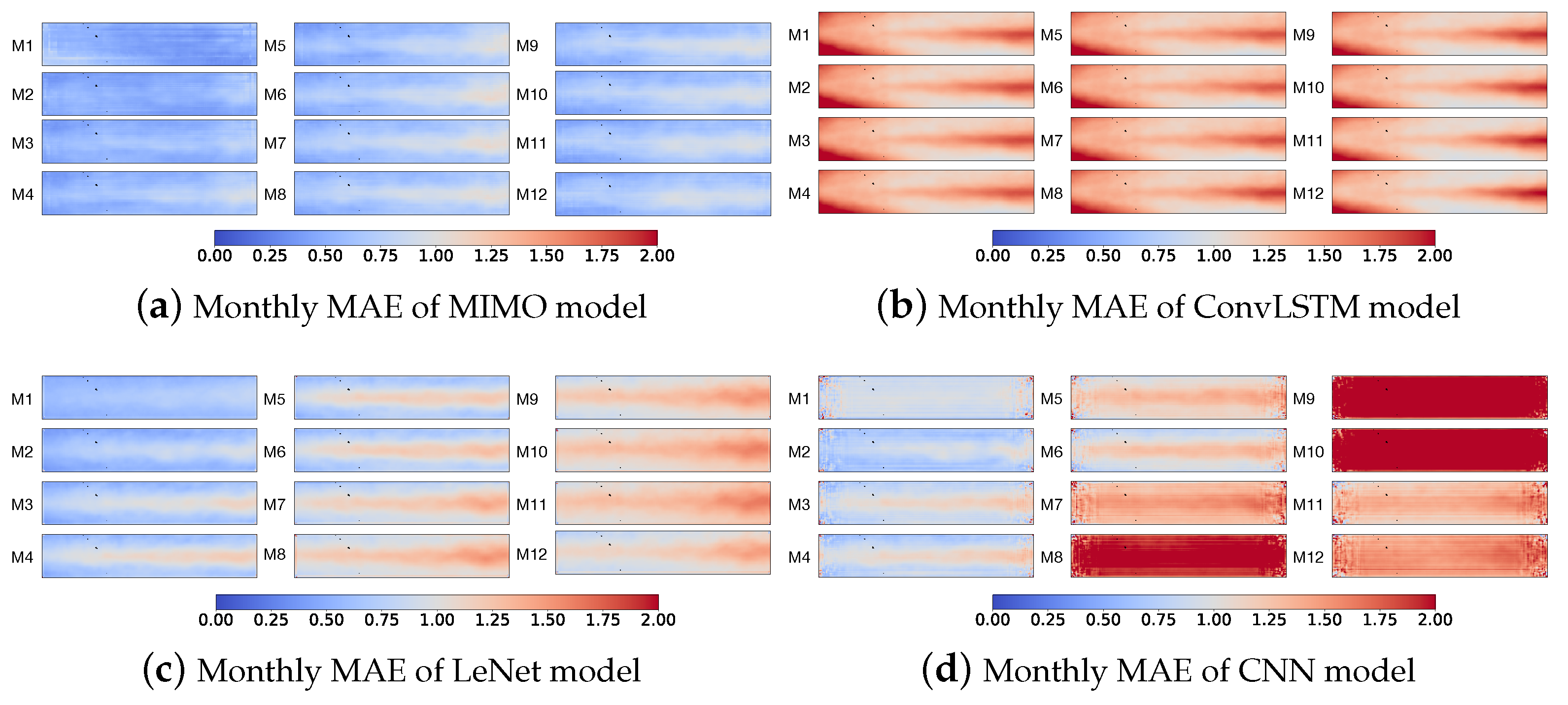
To better demonstrate the effectiveness of the MIMO model, we visualize the mean absolute errors of MIMO, ConvLSTM, LeNet and CNN for daily, weekly and monthly SST prediction in Figure 9, Figure 10 and Figure 11, respectively.

As shown in Figure 9, MIMO and LeNet have similar MAE in daily SST prediction. The MAE of these two models is less than 0.5 for most grid regions. In contrast, the MAE of ConvLSTM is quite large. As for CNN, the predicted results for the 4th, 8th and 11th days are also bad.

Figure 10 illustrates the MAE for weekly SST prediction. MIMO has the best prediction performance among four models and its MAE errors are less than 0.5 for most grid regions. With the increase of time, the MAE of LeNet becomes large and reaches 1.25 for some grid regions. The MAEs of ConvLSTM and CNN are still very large but CNN performs better than ConvLSTM.

Figure 11 illustrates the MAE for monthly SST prediction. MIMO also achieves the best prediction performance. For LeNet, the MAE becomes larger than that of weekly SST prediction and still outperforms ConvLSTM and CNN. The MAE errors of ConvLSTM and CNN even reach 2.0 for some grid regions.

In sum, in accordance with Figure 9, Figure 10 and Figure 11, the MIMO model can achieve quite good prediction performance in all daily, weekly and monthly SST prediction. LeNet also achieves good prediction performance on daily SST prediction but has larger prediction errors than MIMO in weekly and monthly SST prediction. Both MIMO and LeNet largely outperform ConvLSTM and CNN.

5.4. Discussion

According to the experimental evaluation, the proposed MIMO model achieves good performance in predicting SSTs of different temporal scales and outperforms multiple classical forecasting methods. The underlying principles can be explained from two aspects.

On the one hand, the dynamics of SST has short-term temporal dependency, middle-term trend and long-term periodicity. For short-term temporal dependency, the SST in the next few days is usually similar to the that of past few days. For the middle-term trend, the SST may keep increasing within a few weeks. For long-term periodicity, the SST of the same month in two consecutive years is often similar. Therefore, integrating SST predictions of different temporal scales lets us have a better understanding of the dynamics of SST from an overall review and could further enhance the prediction performance.

On the other hand, the SSTs of different temporal scales are often correlated. For example, the increase of short-term SST causes the ocean to accumulate energy, which will result in the changes of long-term SST. Meanwhile, when the energy is accumulated to a certain extent, the ocean begins to release energy. Therefore, long-term SST changes will also affect short-term SST. The proposed MIMO model can fully take advantage of such correlations to improve SST prediction.

6. Conclusions

This work proposes the multi-scale SST prediction problem and develops a new model named Multi-In and Multi-Out (MIMO) to address this problem. MIMO can fuse multi-scale SST data and external data to learn comprehensive features and decode the learned features to adaptively predict daily, weekly and monthly SST. Experimental evaluation shows that MIMO can achieve much better prediction performance than existing SST prediction methods in predicting weekly and monthly SST, and comparable prediction performance with the state-of-the-art prediction method in predicting daily SST. The superiority of MIMO lies in that it can do multi-scale SST prediction in a unified model, thus improving the prediction accuracy by capturing the correlations among different scales of SST.