Article

The Spatiotemporal Change of Glacier Runoff Is Comparably Attributed to Climatic Factors and Physical Properties in Northwestern China

1
State Key Laboratory of Urban and Regional Ecology, Research Center for Eco-Environmental Sciences, Chinese Academy of Sciences, Beijing 100085, China
2
University of Chinese Academy of Sciences, Beijing 100049, China
*
Author to whom correspondence should be addressed.
Remote Sens. 2022, 14(10), 2393; https://doi.org/10.3390/rs14102393
Submission received: 8 March 2022 / Revised: 5 May 2022 / Accepted: 13 May 2022 / Published: 16 May 2022
(This article belongs to the Topic Cryosphere: Changes, Impacts and Adaptation)

Abstract

:
The spatiotemporal regimes of glacier runoff (GR) under a warming climate are of great concern, especially in dryland areas in northwestern China (DAC). Due to the difficulty of observing GR, little attention has been given to the spatiotemporal change in GR at regional scales. This study uses the regional individual glacier mass balance (GMB) dataset developed by digital elevation models (DEMs) to simulate the spatiotemporal regime of GR using atmospheric parameters considering both ablation and accumulation processes on glaciers. In this study, GR, including glacier meltwater runoff (MR) and delayed water runoff (DR) of the DAC, was quantitatively assessed at a catchment scale from 1961 to 2015. The total annual GR in the DAC was (100.81 ± 68.71) × 108 m3 in 1961–2015, where MR accounted for 68%. Most basins had continuously increasing tendencies of different magnitudes from 1961 to 2015. The least absolute shrinkage and selection operator (LASSO) and random forest techniques were used to explore the contributions of climate factors and glacier physical properties to GR, and the results indicated that climate factors could explain 56.64% of the variation. In comparison, the remaining 43.36% could be explained by the physical properties of glaciers themselves (i.e., degree-day factor on ice, degree-day factor on snow, glacier median height, aspect, and slope). This study not only improves our understanding of the spatiotemporal change in GR in the drylands of northwestern China at spatial and temporal resolutions but also highlights the role of physical properties in explaining the heterogeneous dynamics among GRs unlike previous studies that only emphasize rising temperatures.

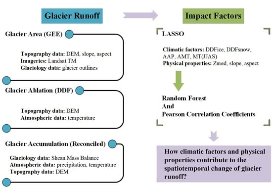
Graphical Abstract

1. Introduction

Glaciers and ice sheets, which store most of the ice and snow on Earth, are known as the largest reservoirs of freshwater [1,2]. Glaciers release meltwater in wet seasons, carrying precious freshwater downstream of glacierized basins and thus alleviating drought [3,4,5] and poverty [6,7], which in turn affects socioeconomic development [8,9,10,11]. Climate change has spurred rapid changes in the cryosphere [5,12,13,14,15,16]. Additionally, the interactions between the cryosphere and the atmosphere and anthroposphere are increasingly intensifying, being especially prominent for hydrological processes, ecosystems [17,18], and the sustainable development of the human economy and society. By the end of the 21st century, one-third of glacierized drainage basins might experience runoff decreases of greater than 10% due to glacier mass loss, with the largest reductions occurring in central Asia [19]. Understanding the dynamics of snow and ice, particularly at the regional scale, is a scientific requirement to meet targets of the Sustainable Development Goals (SDGs) [20,21,22,23,24,25] and two goals of the Intergovernmental Science-Policy Platform on Biodiversity and Ecosystem Services (IPBES) [26,27,28,29,30].
Most river basins in dryland areas of northwestern China (the DAC) depend heavily on GR, which is a high-altitude water resource [31,32,33,34], and GR supports 90 percent of local residents by providing water for oasis agriculture areas (OAAs) [35,36], such as that in the Hexi Corridor (2.17 × 10⁴ km2) [37]. Under high demand for water as a result of a rapidly growing population and irrigation combined with the arid climate of the DAC [8,38,39], the importance of water provided by glaciers in arid regions is apparent [4,16,38,40].
Accurate and detailed glacier mass balance (GMB) data are obtained through continuous field observation, which provide a deeper understanding of glacier–climate and glacier–hydrology interactions and are the basis for glacier-related modeling verification [41,42]. Due to field observations’ financial and logistical difficulties, it is common to calculate continuous GMB for long time series at a regional scale [43,44]. However, only 40 glaciers, which are internationally called “climate reference” glaciers, have been consistently monitored long enough to measure changes under climate change, while none of them are located in the DAC, indicating a lack of long-term mass balance observations for this region. At the regional scale, degree-day factor models are widely used to calculate glacier runoff (GR) driven by the atmosphere based on meteorological data recorded by meteorological stations [45,46]. Nevertheless, the degree-day factor model is limited by the number of meteorological stations available, and the model does not fully restore the two processes of glacier ablation and accumulation.
In recent decades, many studies have used methods including in situ measurements, remote sensing, or modeling to explore glacier change and its influencing factors [5,12,13,14,15,16], with most focusing on the effects of atmospheric factors on GR [33,47,48]. Some studies generally indicate that glacier shrinkage is mainly caused by a significant increase in temperature [33,48]. Increases in precipitation have been observed in most glacial areas of China, while these precipitation increases are far from offsetting the impact of temperature [49,50]. However, few studies have described the influence of glacier physical properties on GR [5]. Studies have shown that physical properties also significantly impact GR in addition to atmospheric driving factors, so this paper presents a comprehensive analysis of climate and physical properties.
Taking advantage of the development of digital elevation models (DEMs), high-resolution mass balance datasets have been published, enabling the estimation of high-resolution GR data [43,44]. Although still limited by time series, the GMB dataset provides an opportunity to explore the influencing factors of the dynamics of glaciers at a large regional scale. This study first used the mass balance model and high-resolution mass balance dataset to restore atmospheric-driven glacial accumulation by correcting precipitation at high altitudes. Then, the degree-day factor model was used to calculate the glacier ablation process to obtain the runoff time series generated for the glacier region from 1961 to 2015. Second, we verified the quantity or trend of GR at the watershed scale from existing studies [15,25,37,38,51,52,53]. Glaciers were classified according to the variation trend and time point of significant change in GR, and the composition of glaciers in each basin was obtained. After exploring the consistency of the change trend of GR with that of temperature and precipitation, the least absolute shrinkage and selection (LASSO) and random forest techniques were used to identify climatic factors (precipitation and temperature) and physical properties of glaciers themselves (slope, aspect, altitude, etc.) to calculate the contribution rates of various factors to GR. Climatic factors were identified based on factors taken into account in the glacier model of Huss et al. (2018). The angle of a glacier could divide glaciers into debris-free glaciers and debris-covered glaciers, and the elevations of the glaciers corrected the temperature on glaciers. The time series of GR and the influence of atmospheric factors and physical properties on GR can benefit the cryosphere science, ecology, hydrology, climate change, and social and economic development of each glacierized basin, providing a scientific basis for decision-making on regional sustainable development.

2. Materials and Methods

2.1. Observations

The sources of data used in this study are listed in Table 1 and are accessible at the given websites.

2.2. Study Area

Data for the DAC region were obtained from the aridity index supported by the United Environment Programme (UNEP), excluding the range of the Tibetan Plateau, which should be discussed separately because of its unique characteristics. There are eight glacier regions around the DAC, including approximately 42,000 glaciers affecting 22 tertiary watersheds. Specific glacier region and tertiary watershed names are listed in Table 2. These watersheds cover different arid zones in the DAC, including hyperarid regions (AH); semiarid and arid regions (SA); and semiarid (S), arid (A), and hyperarid zones (SAH). The study area is shown in Figure 1 along with the abbreviations used in this study.
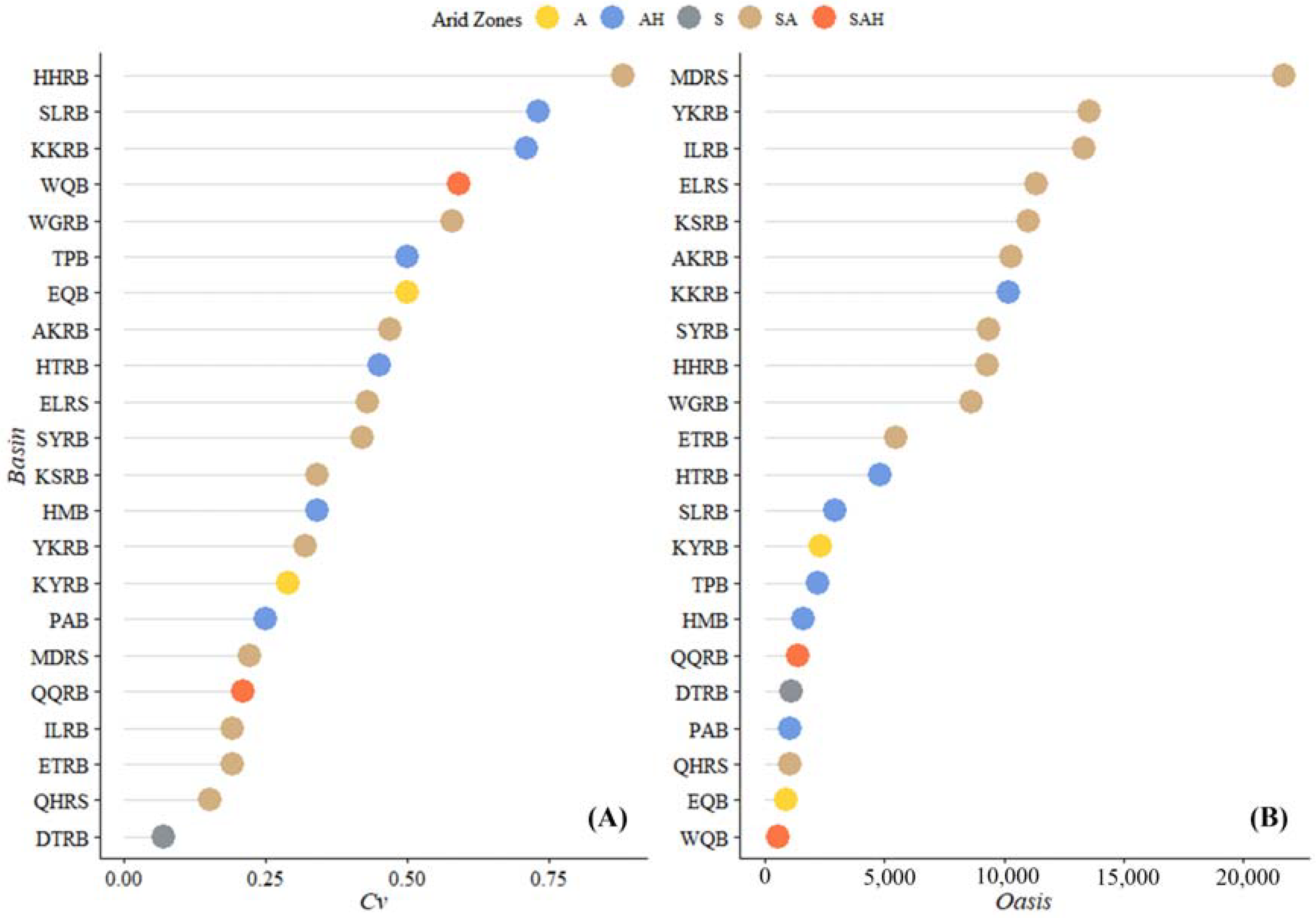
Figure 2 shows the coefficient of variation of precipitation (Cv) (Figure 2A) and the area of OAAs (Figure 2B) for each watershed in the DAC. The area of OAAs in each watershed in the DAC reached a maximum of 21,699.18 km2 (MDRB), with an average area of 6543.69 km2, while the Cv of precipitation in the DAC reached a maximum of 0.88 (HHRB), with an average statistic of 0.40, showing that sources of precipitation were unstable and highlighting the importance of stable meltwater runoff (MR) provided by GR in our study areas. The oasis is the most important area for the livelihood of residents in drylands. A stable water source will affect the livelihood and economic development of the whole region. The coefficient of variability of rainfall in arid regions is so great that the relatively steady flow of water provided by GR is even more valuable.

2.3. Methods

2.3.1. Glacial Accumulation

We imported the maximum precipitation height ( H p r e _ m ) and precipitation gradient ( P G ) to calculate glacier accumulation according to previous studies [54,55,56,57]. We assumed that precipitation lapsed negatively with the specific P G from its actual height to its H p r e _ m . As the RGI provided each glacier’s outline, the equation for reconciling high-altitude precipitation ( P r e c o n ) is shown in Equation (1):
P r e c o n = P A P H × [ 1 + | ( H H p r e _ m ) | × P G × 0.01 ]
where P A P H (m) is the precipitation from APHRODITE, H (m) is the altitude from the DEM at a grid scale, P G (% m−1) is the vertical precipitation gradient for each glacier as a constraint factor, and H p r e _ m (m) is the maximum precipitation height of each glacier region based on previous studies [54,55,56,57].
The calculation of glacial atmospheric accumulation depends on temperature. We divided precipitation into solid (snow) and liquid (rain) by a temperature set to 4 °C, T 1 (°C). Glacial accumulation can be calculated using Equation (2) [58,59]:
A c = { P r e c o n , T a 0 ( 1 T a 4 ) P r e c o n , 0 < 0 , T a > 4 T a 4 ,  
where T a (°C) is the actual temperature adjusted by a commonly used temperature lapse rate (0.65 °C/100 m) over the glacier area within each grid cell, P r e c o n (m) is the reconciled precipitation based on Equation (1), and A c (m) is the accumulation on a glacier.

2.3.2. Glacial Ablation

The degree-day factor ( D D F ) model is a common method used to obtain glacier ablation, as shown in Equations (3)–(5):
A b = D D F × P D D ,
P D D = t = 1 n H t · T a , t
H t = { 1 , T a , t 0 0 , T a , t < 0
where P D D are positive-degree days, H t is a logistic variable, t refers to the time scale, and T a , t is the temperature adjusted by a commonly used temperature lapse rate (0.65 °C/100 m) over the glacier area within each grid cell. It is worth mentioning that monthly positive-degree days ( P D D m ) were used in this paper, namely, the sum of daily positive-degree days temperature. Based on the field observations of 40 glaciers in western China, Zhang et al. (2006) established the spatial distribution of D D F with a spatial resolution of 0.5 degrees, revealing that D D F had great spatial heterogeneity [60]. The value of D D F increased gradually from northwest to southeast, consistent with the change in hydrothermal conditions from northwest to southeast in western China.

2.3.3. Mass Balance

We used the regional available GMB dataset to constrain high-altitude precipitation. The glacier mass balance (m w.e.) was computed by multiplying mean glacier elevation change, glacier area, and the density of water, where the density of water was 1000 kg/m3 and the water equivalent (m w.e.) was equal to the thickness (m). B y is the sum of accumulation, A c , y (m), and ablation, A b , y (m), at a yearly time step for each glacier following Equation (6):
B y = A b , y + A c , y
We compare datasets from Brun et al. (2017) (Brun Mass Balance), Shean et al. (2020) (Shean Mass Balance), and NASA’s Ice, Cloud and Land Elevation Satellite (ICESat) data (ICESat Mass Balance) in Supplementary Materials Table S1 and Supplementary Materials Figure S1 [61,62,63]. The Shean Mass Balance dataset was used to simulate mass balance using each glacier’s mass balance and uncertainty based on multisource glacier inventory RGI v6.0.

2.3.4. Precipitation Gradient

Limited by the time range of the APHRODITE and Shean Mass Balance datasets, the annual yearly glacier ablation from 2000 to 2015 could be calculated following Equations (3)–(5). Each glacier’s annual mass balance ( B y ) was provided by the Shean Mass Balance dataset. We substituted B y into Equation (6) to obtain the annual accumulation A c on each glacier in the same period. The P G on each glacier could be obtained by substituting A c into Equations (1) and (2). Since the resolution of the APHRODITE dataset was much larger than 100 m, the distribution of P G at regional scales was aggregated using the nearest neighbor algorithm to reduce the impact of grid mutation [64].

2.3.5. Glacial Runoff

By substituting the map of P G , original precipitation, and temperature from the APHRODITE dataset and DEM into Equations (1)–(6), the time series of mass balance for each glacier can be obtained.
Specifically, GR, including MR and delayed water runoff (DR), in this study, was runoff generated within the glacier range, where glacier areas change over time. DR resulted from the remaining precipitation stored as snow in cold seasons and discharged in warm seasons after offsetting ablation [3,40,44], including part of the precipitation in warm seasons. MR, also called excessive MR or the imbalanced part of GR, resulted from the mass loss of glaciers when atmospheric accumulation could not offset glacier ablation.
GR, G m (m), during warm seasons was calculated according to the proportion of monthly P D D , P D D m to yearly P D D , P D D y and the absolute value of yearly mass balance at each grid cell of 100 m with Equation (7):
G m = | B y | × P D D m / P D D y
The monthly DR, D m (m), was measured as the product of B y greater than zero and the proportion of P D D m to P D D y . Accordingly, MR, M m , was measured as the product of B y less than zero and the proportion of P D D m to P D D y as shown in Equations (8) and (9):
D m = B y × P D D m / P D D y ,   B y 0
M m = B y × P D D m / P D D y ,   B y < 0
In this paper, we present a means to obtain a time series of GR, including DR and MR, generated for glacier regions after reconciling high-altitude precipitation using the Shean Mass Balance dataset, which makes up for datasets incomprehensive (only mass balance) or semiquantitative (only GR proportion) for glacier areas at a regional scale. This dataset can be used in hydrological models to better simulate the whole hydrological process.

2.3.6. Glacial Area

We used Landsat TM scenes from Google Earth Engine (GEE) to extract glacier outlines at the end of ablation seasons (September to November in the DAC) in each watershed for 1985–1995 and 1995–2005 by applying band ratio segmentation (red band/midinfrared band, 2.0 as the threshold) [41,65,66]. A 100 m buffer of the glacier outline of the RGI was used as the basic extraction region. The DEM from GEE was used to calculate the terrain slope, while a value of 24 was used as the threshold to distinguish debris-free glaciers from debris-covered glaciers [2]. After classifying dates of Landsat scenes used in the RGI, we determined to use the RGI as the glacier outline for 2000–2015 (Supplementary Materials Table S2 shows the time periods of scenes used in the RGI for different basins).

2.3.7. Total Uncertainty Analysis

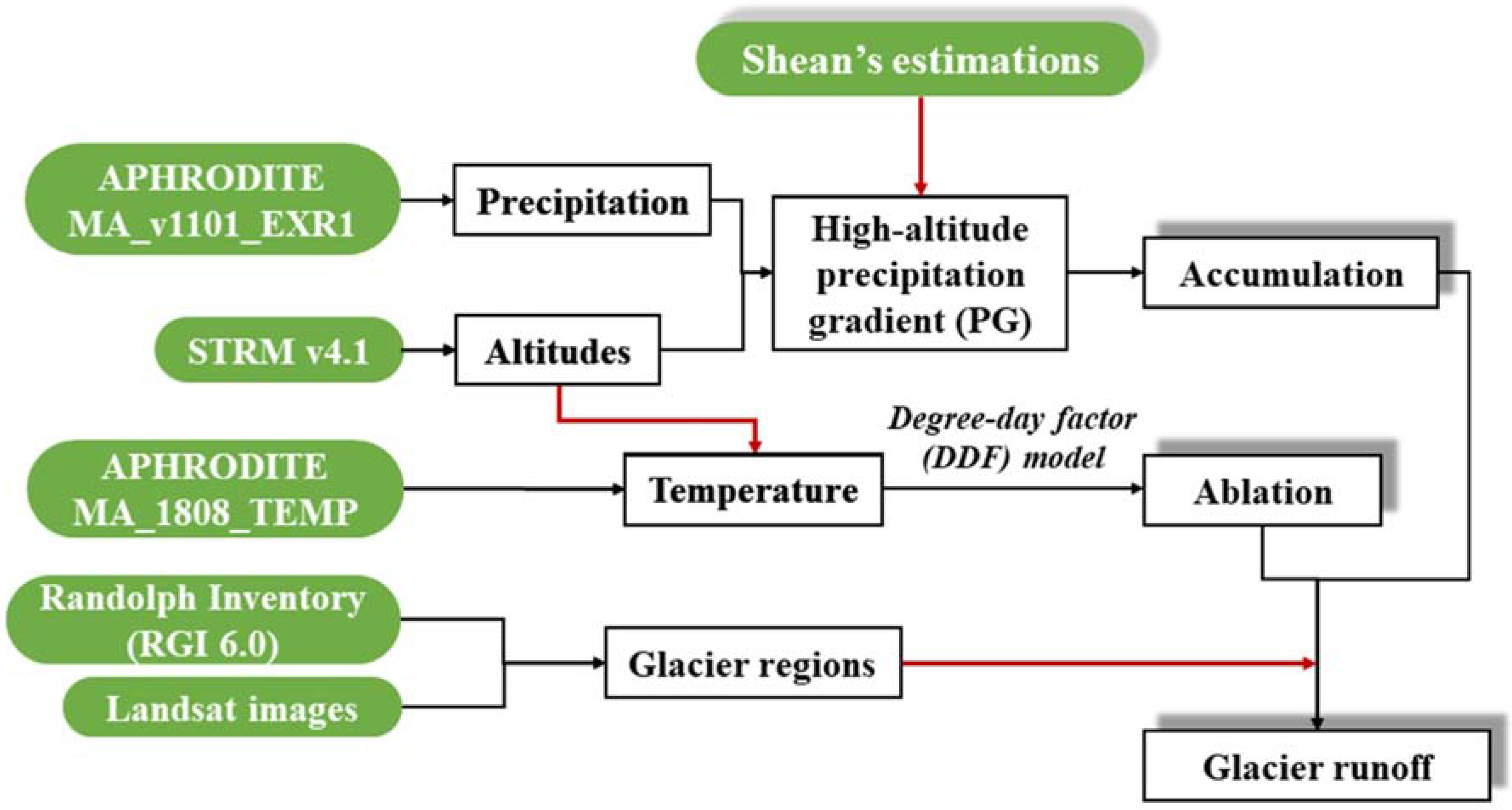
The individual glacier uncertainty (including random and systematic errors) calculated in the Shean Mass Balance dataset denotes the uncertainty range of GMB changes. Using the same routine that we described in Section 2.3.4 to calculate the distributions of P G corresponding to the maximum and minimum mass balance values from the Shean Mass Balance dataset, the time series of the maximum and minimum GR generated by the map of the corresponding P G were obtained by substituting the original precipitation and temperature levels from the APHRODITE dataset and DEM into Equations (1)–(9). The calculations of DR and MR and their uncertainties are shown in Figure 3, where shaded blocks are the calculated results with uncertainties.

2.3.8. Trend Analysis

The temporal trends of annual GR, DR, and MR in the DAC were tested using the Mann–Kendall (MK) test [67,68]. Given a time series x ( t ) with length n , the statistics denote that the data series is an independent random variable with the same distribution composed of n elements.
d k = i = 1 k m i
m i = { 1 , x j > x i 0 , x j x i
where m i represents the cumulative number of x ( i ) greater than x ( j ) ,   1 j i ,   1 k n .
E ( d k ) = k ( k 1 ) / 4
V a r ( d k ) = k ( k 1 ) ( 2 k + 5 ) / 72
where mean E ( d k ) and variance V a r ( d k ) are calculated and 1 k n .
After standardizing d k , U F k and U B k can be obtained from Equations (14) and (15):
U F k = d k E ( d k ) v a r ( d k )
U B k = U F k
The intersection point of the U F curve and U B curve in the confidence interval was determined as a turning point. An increasing trend of a time series was found when U F > 0 ; in contrast, a declining trend of a time series was observed when U F < 0 .

3. Results

3.1. Glacial Area Change

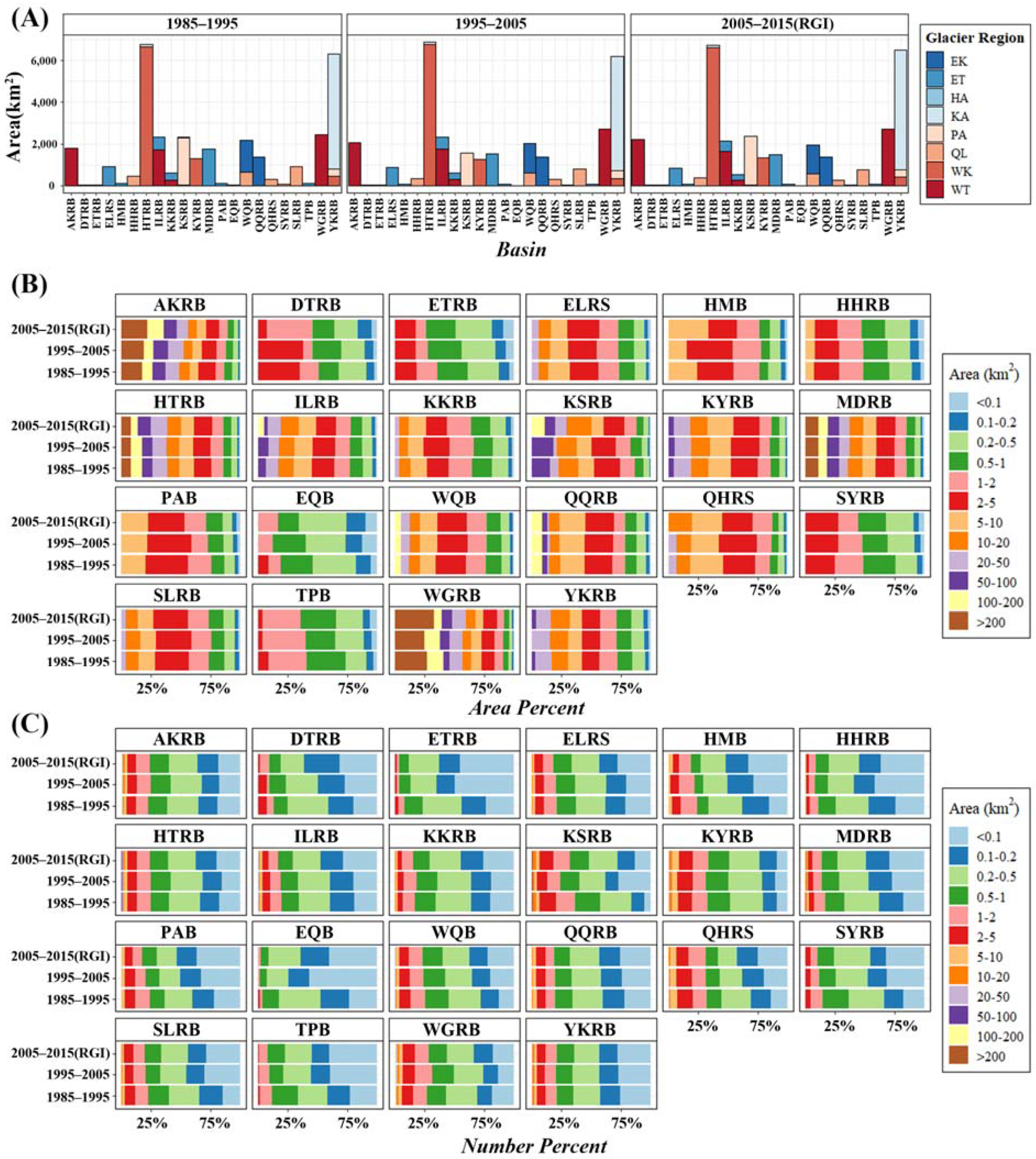
In the RGI, 53,749 glaciers were found with a total area of 32,008 km2 in our study area. The HTRB had the largest glacier area (6719.50 km2), and the YKRB had the most significant number of glaciers (4487). Figure 4A shows the glacier area in each watershed originating from different glacier regions in three periods (1985–1995, 1995–2005, 2005–2015). The general characteristics of glacier size distribution are that large numbers of small glaciers account for a small proportion of the total area, while fewer large glaciers account for a large proportion of the total area [41,65,69,70,71]. This feature is also evident in our study area, especially in the AKRB, HTRB, and WGRB, as shown in Figure 4B,C. Glaciers in the DAC are mainly less than 1 km2, accounting for 70% or more of the total glacier area in the corresponding basin. Except for the DTRB, ETRB, EQB, SYRB, TPB, and ELRS, glaciers larger than 2 km2 account for 50% or more of each basin.
The area proportion of glaciers in the YKRB is controlled by the KA, QQRB, and WQB, where the EK controls remain almost unchanged, as the KA, referred to as the “Karakoram anomaly” [55], remains relatively stable, and the EK has a positive mass balance [43,44]. The area proportion of glaciers larger than 5 km2 in the QKRB, HTRB, ILRB, KSRB, MDRB, and WGRB, controlled by large glaciers, increases with each period. The area proportion of glaciers smaller than 1 km2 in the HHRB, EQB, SYRB, and ETRB increases period by period. The higher area proportions of >1 km2 glaciers in these basins also illustrate the dominance of small glaciers.

3.2. Glacial Runoff from 1961 to 2015

In this study, the Shean Mass Balance dataset was used to reconcile high-altitude precipitation. The yearly mass balance of glaciers influencing the DAC from 1961 to 2015 was calculated from the difference between accumulation obtained from corrected precipitation and ablation calculated by the DDF model. We created a long-time series dataset of the total GR dataset, including DR and MR, based on atmospheric hydrothermal conditions at large regional scales with a spatial resolution of 100 m. It is worth noting that GR in this paper refers to the runoff generated within the geographical area of a glacier or the runoff generated under the glacier area of different time ranges extracted from GEE based on the RGI. GR included DR, which was stored rainfall in the cold seasons and released runoff in the ablation seasons, while MR resulted from glacier mass balance, which is also called excessive MR or the imbalanced part of GR. The GR in each basin from different glacier regions in the DAC is shown in Figure 5. The average GR in the DAC for the period was (100.81 ± 68.71) × 108 m3, where MR accounted for 68%. MR largely controlled basins affected by the DAC’s glaciers.
We used the ratio of DR to GR to estimate the health and sustainability of glaciers in the DAC, as reported by Miles et al. (2021) [72]. The GR in the HTRB, KYRB, YKRB, and QQRB influenced primarily by the KA, WK, and EK with positive mass balance estimated was judged healthier than that in the other glacierized basins in the DAC, with more than 50% of GR consisting of DR brought by precipitation. In contrast, the GR in other basins, including the ELRS, ILRB, and MDRB (the largest OAAs in the DAC), was nearly entirely MR, indicating that measures to adapt should put environmental and cryosphere changes in these basins forward as soon as possible.
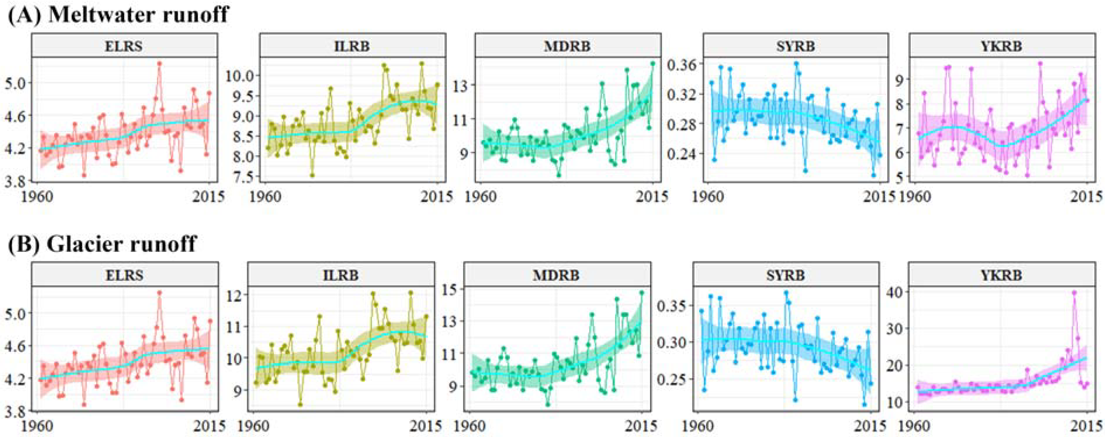
Figure 6 shows the time series of MR and total GR in basins with the top four OAAs and SYRB after Loess smoothing. Locally estimated scatterplot smoothing (LOESS) and locally weighted scatterplot smoothing (LOWESS) are two nonparametric regression methods developed for scatterplot smoothing. When there is only one independent variable and no prior weights, the functions “LOESS” [73] and “LOWESS” [74] in R language programming are equivalent, in principle. In the past 50 years, except for the DTRB, HHRB, and SYRB, the runoff of the other basins showed a continuously increasing trend, although periods of significant increase differed. The MK test showed that the GR in the ELRS and KKRB increased significantly after 2000, while KSRB and HTRB levels increased significantly after 1980. In the DTRB, GR began to decrease after 1990, while in the HHRB, it began to decline after 1995, but neither decreased significantly before 2015. Only the GR series in the SYRB began to decline after 2000 and significantly reduced after 2010, as the results of the MK test showed, and the trend was consistent with previous studies [75]. The MK value and time series of DR, MR, and total GR for all basins are illustrated in Supplementary Materials Figures S2–S6.

3.3. Sustainability of Glaciers in the DAC

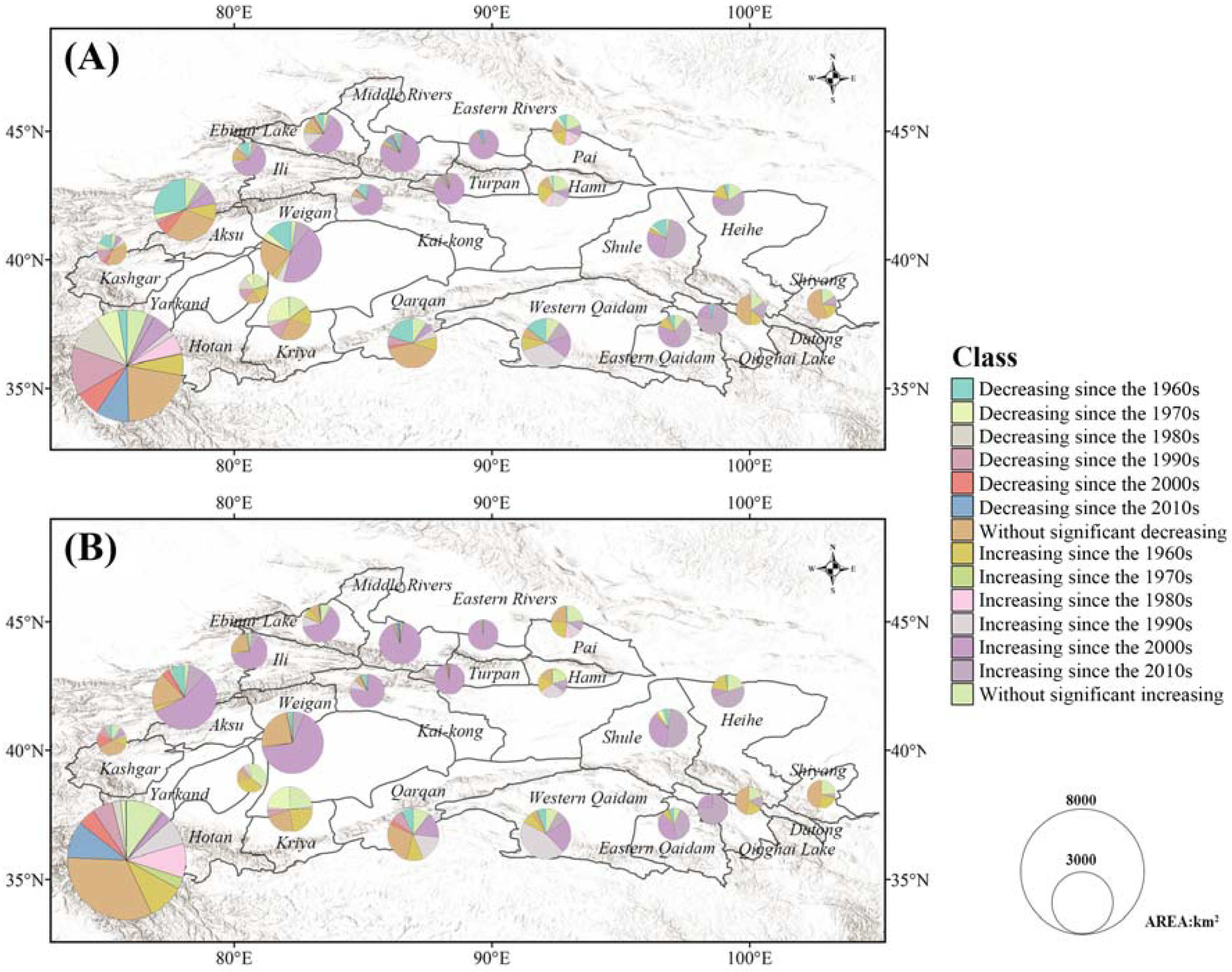
The time series of glacial MR for the past 55 years for each glacier was counted based on the RGI, and the MK test was conducted for each MR series to obtain statistics of the change trend and the time when significant changes occurred for each glacier. The classification of glaciers in each watershed in the DAC was guided by the results of the MK tests, while glaciers were divided into 14 categories, including those that expanded or reduced significantly since the 1960s, 1970s, 1980s, 1990s, 2000s, and 2010s and varied without significant increase or decrease in the past 55 years. The numbers and areas of the composition and distribution of different glacier types in each basin are shown in Figure 7A,B.
The areas and numbers of glaciers in different basins directly determined glacial trends. For example, in the SYRB, over the past 55 years, both the numbers and areas of glaciers almost all showed a declining trend, resulting in a declining GR in the basin. Glaciers in the YKRB exhibited varied patterns of expansion and contraction in different periods. Although the numbers and areas of glaciers without a significant decrease accounted for 72.24% and 56.97% of the total amount and area of glaciers in the whole basin, respectively, the MR in the YKRB was still on the rise and reached a significant level after 1995. This suggests that the trend of MR could only be assessed by fully considering the mass balance of each glacier in the basin in addition to the area and amount ratios and significant time points.
Establishing the relationship between MR and air temperature is a common means to calculate MR and reflects the dominant role of temperature in meltwater [12,45,75,76]. The MK test was also used for temperature, and the composition of different temperature changes was obtained using the same classification method as that of MR. The results showed that the number and area of glaciers with the same trends of temperature and MR accounted for 27.12% of the total number and area of all glaciers. Considering the lagged influence of temperature on MR (5–10 years) [76], the number and area of glaciers with trends of temperature and MR in coordination accounted for 31.68% of all glaciers. Due to the findings not reflecting a strong correlation between temperature and MR, we attempted to clarify the factors affecting MR and the respective explanatory rates.

3.4. Climatic Factors and Physical Properties Explain the Spatiotemporal Patterns of GR

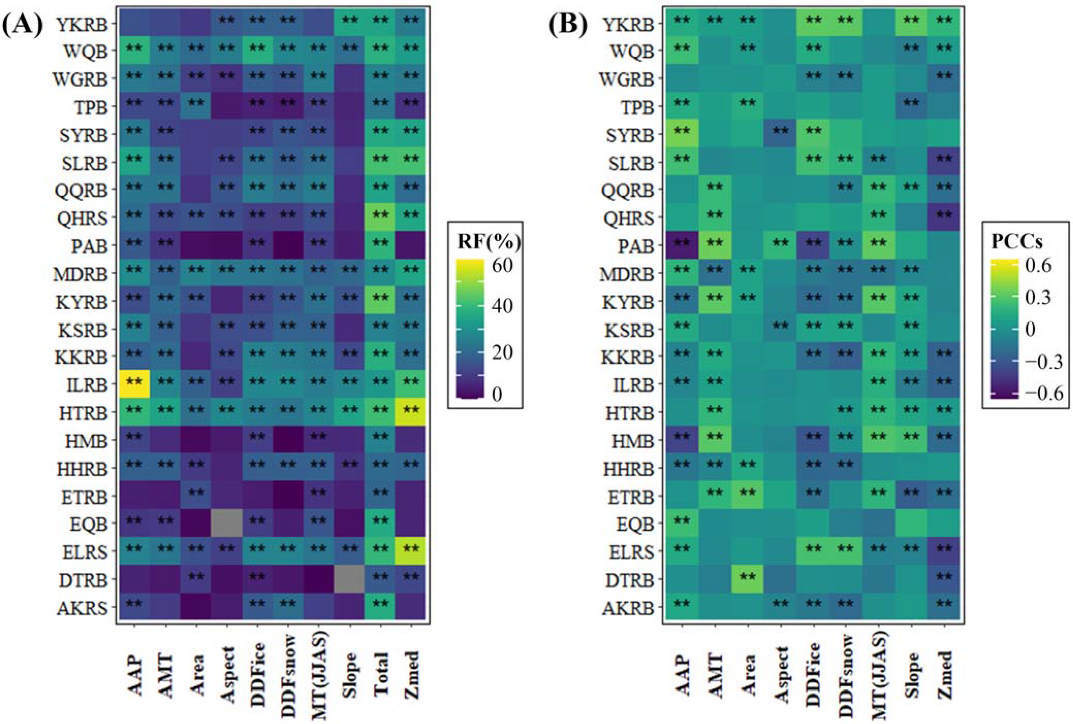
To find the impact factors of MR, a linear model with variable selection based on the LASSO operator was used to select a subset of potential MR predictors that could reduce predictors by decreasing the estimated regression coefficients toward zero to avoid an overfitting of the models caused by high-dimensional problems. The coefficients and significance of the MR predictors for each river basin based on the LASSO regression method are shown in Supplementary Materials Table S3. The correlations between MR and normalized potential predictors (the degree-day factor on ice (DDFice), the degree-day factor on snow (DDFsnow), median glacier height (Zmed), aspect, slope, annual average precipitation (AAP), annual mean temperature (AMT), mean temperature in wet seasons (MT(JJAS)), and area) after the LASSO regression were analyzed for each basin. Additionally, the RF technique was used to calculate the relative rate of the contribution of the potential predictors with significance based on a large number of decision trees (in this study, 500) fitted to random subsets of the training sample. Both the results of the RF and Pearson correlation coefficients (PCCs) are shown in Figure 8.
The MR predictors were obviously different in different basins. The PCCs of AAP in the HMB and PAB were −0.39 and −0.56, respectively, while the PCCs in the WQB, EQB, SYRB, and SLRB were 0.24, 0.38, and 0.25, respectively. Among all basins where AMT dominated, there was a significant positive correlation, with coefficients of 0.22 in the QQRB, 0.21 in the HTRB, 0.22 in the QHRS, and 0.32 in the KYRB. The absolute PCC of Zmed was the highest among all predictors in all basins, with a coefficient of 0.17, followed by DDFice and AAP, with coefficients of 0.16, and the absolute PCC of AMT and MT(JJAS) was 0.13. The RF results showed that the overall explanation rate of the nine potential predictors of MR selected by LASSO was 31.49 ± 14.97% in the DAC. The explanatory rates of Zmed and AAP in each watershed were 32.40 ± 27.14% and 29.39 ± 26.09%, respectively. AAP accounted for 59.53% of the MR in the ILRB, and Zmed accounted for 55.47% and 53.42% of the MR in the HTRB and ELRB, respectively. Overall, climate factors could explain 56.64% of the MR, while physical factors, including DDF, aspect, slope, Zmed, and area, could explain 43.36% of the MR, showing that the MR of continental glaciers was not only related to the hydrothermal conditions, especially precipitation and temperature in wet seasons [77,78,79,80,81], but also greatly related to the physical properties of glaciers themselves. In other words, the explanatory rates of climate and physical factors among the potential predictors of MR were relatively consistent. When considering glacier MR, the physical properties of glaciers themselves should be taken into account, and spatial heterogeneity should be considered when climate factors are considered based on climate factors considered in previous studies.

4. Discussion

4.1. Precipitation Correction at High Altitudes

Glaciologists and meteorologists have long debated whether mountains have one or two maximum rainfall heights [18,53,54,82,83,84,85]. Even in the same location, H p r e _ m varies across the seasons observed and data and methods used. For example, the APHRODITE dataset and the GPM show H p r e _ m at 4200 and 2600 m in the Junggar Basin, respectively, and at 2750 and 4050 m in the Northern Tarim Basin, respectively [86]. Bai et al., found that in the summer on the northern slope of Tien Shan, the median height of H p r e _ m was 2100 m, while in the winter, it was 1100 m, and the average height was approximately 3000 m, consistent with Zhang et al. (2019) [18,83].
Horizontal precipitation, such as fog, frost, and dew, can be seen in mountainous areas year-round, especially in areas above 3500 m. After condensation, the underlying surface picks up this water vapor. Nevertheless, standard rain gauges commonly used for meteorological observations cannot capture it, which results in a deviation in the precipitation record of the rainfall gauges for high mountains, whether the rainfall gauge is correct in recording precipitation in high mountain areas directly affecting rainfall correction in mountain areas or not. Therefore, P G was calculated according to the average regional H p r e _ m in this paper, and H p r e _ m was used as the calculation standard in this paper. The H p r e _ m of each glacier area was shown in Table 3.

4.2. Comparison of GR Estimations

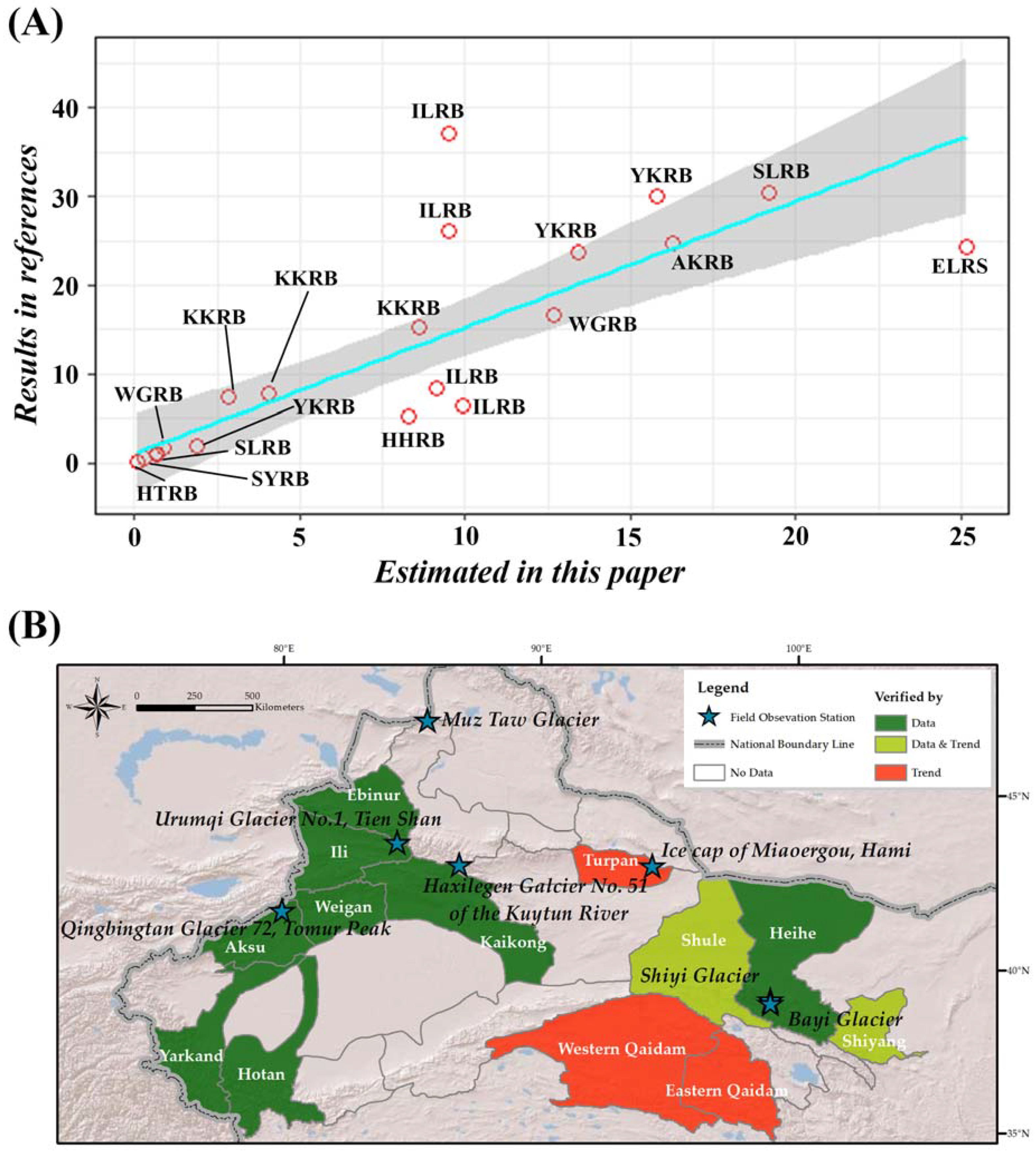
Some studies [15,25,37,38,51,52,53] have simulated the GR in the DAC by qualitative or semiquantitative methods or using hydrological or physical models. We compared our estimations to these results, although there were no numeric data for partial river basins due to there only being trend studies, as shown in Figure 9.
In this paper, scientific references were selected via systematic searches of keywords including the name of each watershed, “glacier runoff”, and “meltwater runoff” using the websites of academic journals (Science Direct, Web of Knowledge, China National Knowledge Infrastructure) to compare the estimated values of the GR obtained in this paper. In total, only 11 of the 22 glacier-derived basins in the DAC [33,51,85,88,89,90,91,92,93,94,95,96] had reference numerical values and GR tendencies [51,97] for the other three watersheds, as shown in Figure 9. Based on these studies, reference numeric values were classified as the GR recharge percentage (four basins), the GR growth rate (four basins), and GR (five basins). The ratio of our results and reference values for the DAC was 0.67. The MR in the HMB showed a slight decreasing trend consistent with our estimate. Hydrological stations in the WQB and EQB showed a sudden change in runoff in 2004, and our estimates show that the turning points of the MR in the EQB and WQB occurred in 2001 and 2002, respectively [87].
The difference between our estimates and previous studies is partly due to the use of different GMB datasets. For example, in the ILRB, GR was measured as 3.72 × 10⁹ m3 by Li et al. [98], which is greatly different from our estimate of 9.5 × 10⁸ m3. Previous studies often deduce the mass balance of a whole region based on the long-term observed mass balance data of a glacier in a certain region while ignoring the spatial heterogeneity of a glacier itself and the hydrothermal conditions it is subject to [94,99]. This method is prone to cause great uncertainty. Another reason for the difference concerns the use of the DDF model which ignores the accumulation process on glaciers [33,76,99]. Amid the current qualitative and semiquantitative analyses of the impact of glaciers on runoff, there is a lack of quantitative research on glacial meltwater, which leaves considerable uncertainty in future predictions for different basins. The model established in this paper can serve as a new method for predicting GR in the future. Of course, field observation is the most accurate means to study glaciers. The establishment of observation systems and continuous hydrological monitoring according to different types and regions of glaciers can further predict the evolution of glaciers and glacial water sources more accurately.

4.3. Implications for the Evaluation and Prediction of GR

Compared to the first Chinese Glacier Inventory (CGI-1) and second Chinese Glacier Inventory (CGI-2), the glacier area in the QL varied greatly in terms of area, altitude, and aspect, and there was obvious longitude zonal differentiation [75]. The DDF model indicates that increased GR is the main cause of the projected increase in total runoff for the upper Indus Basin [100]. However, when glacial ablation and accumulation processes were both considered, the contribution rate of GR to the projected increase in total runoff decreased, changing the pattern of the contribution rate to total runoff to increase. In the same way, while the modified Budyko equation only considers ablation and not accumulation, the finding that accelerated glacier melt contributed to a nearly 80.9% increase in surface runoff in the upper Brahmaputra Basin is overestimated [101]. To improve the estimation of the GMB, glacier physical properties have been taken into account in some studies. In the European Alps, Podsiadlo et al. (2020) extracted glacier surface properties such as slope and aspect and integrated them into a hydroclimatological model to estimate the spatially distributed annual glacier mass balance, confirming the effectiveness of the considered physical properties by in situ observations [102]. After comparing the CGI-1 and CGI-2, Su et al., suggested that both climatic conditions and glacial morphology mainly influence glacier shrinkage in China, while shrinkage manifests in the DTRB (−19.97%), SYRB (−14.21%), and HHRB (−15.67%) [5,41]. In conclusion, the prediction of GR was improved by making full use of the physical properties of glaciers and combining the two processes of glacier melting and accumulation with field measurement data.

4.4. Socioeconomic Consequences

OAAs in the DAC were most dependent on DR for irrigation and the maintenance of agriculture and for maintaining soil moisture, vegetation growth, and groundwater recharge to maintain security [24,103,104]. Twenty-two glacierized basins irrigated 143,939.24 km2 of OAAs, providing water for 14 million people in 19 urban districts. In 2015, the gross domestic product (GDP) of the primary industry in these districts was nearly 111.54 billion US dollars, accounting for 14.1 percent of the total GDP of these districts, double that of the primary industry and accounting for 7 percent of the national GDP. While the real primary industry GDP of the DAC was 40.46 million US dollars, OAAs accounted for 79.86 percent. Increased GR could provide more water for agriculture and livestock to ensure food security and water for residential and industrial use. However, the increase in GR was unsustainable [4,95].
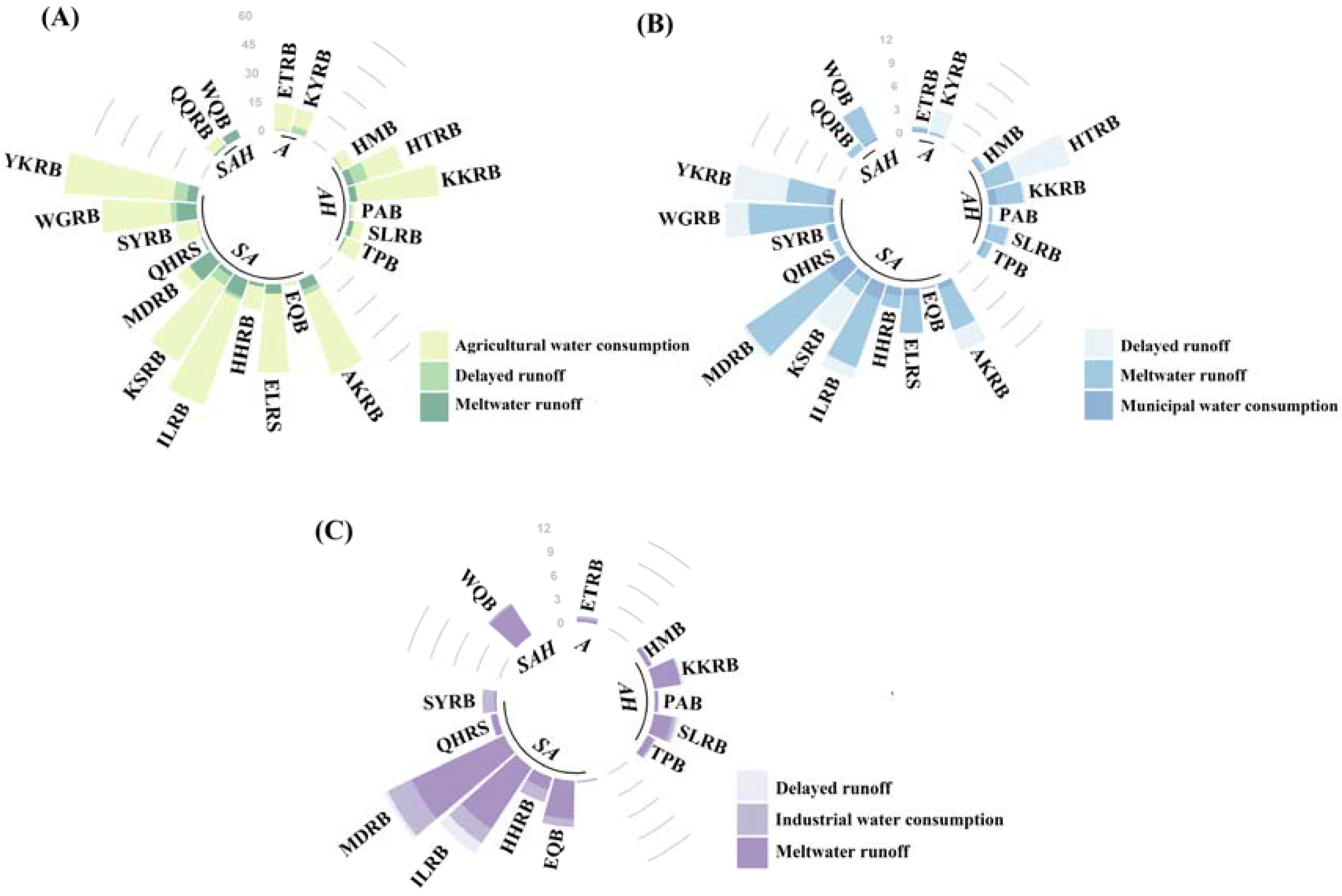
The proportion of GR in agricultural, industrial, and municipal water consumption DAC basins is shown in Figure 10. Agrarian water consumption at the watershed scale was obtained by averaging agricultural water consumption statistical data to land use types of agricultural land and then ranging regional statistics, which were the same as those of industrial and municipal water consumption. Because quantifying the economic and social impacts of cryospheric change is critical to make public policy and impact adaptation decisions, our estimate may support the referentially quantifiable long-term GR time series.

5. Conclusions

This paper overcomes the shortcomings of large-scale geodetic quality assessments. We used the Shean Mass Balance dataset and calculated the precipitation gradient to quantitatively study the seven major glacier regions around the DAC, including nearly 42,000 glaciers. We established the spatiotemporal changes in the GR (DR and MR) in 22 glacierized watersheds with a spatial resolution of 100 m from 1961 to 2015.
1. This paper used the mass balance of the Shean Mass Balance dataset to obtain a high-altitude precipitation gradient with uncertainties and then calculated the long-term time series of GR, including DR and MR, considering both ablation and accumulation processes, while the average total GR in the DAC was (100.81 ± 68.71) × 108 m3. Moderate MR reached (63.44 ± 46.65) × 108 m3 and DR was (37.37 ± 22.06) × 108 m3 in 1961–2015. The ratio of our estimations to existing studies was measured as 0.67, proving the influence of the accumulation process on the estimation of GR.
2. After comparing the number and area of glaciers with the same trend of temperature and MR, the temperature was found to be the most central factor affecting MR, and the lagged influence of temperature on MR did not show a strong correlation between the former two variables. Based on the LASSO and RF results, the contributions of hydrothermal conditions, including temperature and precipitation, and glacier physical properties, including area, slope, aspect, and altitude, to GR were nearly equal. It was effective to improve the estimation of GR by making full use of the physical properties of glaciers and combining the two processes of glacier ablation and accumulation with field measurement data.

Supplementary Materials

The following supporting information can be downloaded at: https://www.mdpi.com/2072-4292/14/10/2393/s1, Figure S1: Mass balance in different glacier regions. Figure S2: Mann-Kendall Test of delayed runoff with a confidence of 95%. Figure S3: Mann-Kendall Test of meltwater runoff with a confidence of 95%. Figure S4: Mann-Kendall Test of glacier runoff with a confidence of 95%. Figure S5: Time series of MR in each watershed. Figure S6: Time series of GR in each watershed. Table S1: Comparison about mass balance datasets in different glacier regions. Table S2: Dates of Landsat imageries used in RGI. Table S3: Coefficients of potential predictor based on LASSO regression method.

Author Contributions

Conceptualization, X.L. and X.F.; Data curation, X.L. and Y.Z.; Formal analysis, X.L.; Funding acquisition, X.F. and B.F.; Investigation, Y.Z.; Methodology, X.L.; Project administration, X.F. and B.F.; Supervision, X.F. and B.F.; Validation, X.L.; Visualization, X.L.; Writing—original draft, X.L. and X.F. All authors have read and agreed to the published version of the manuscript.

Funding

This research was funded by the National Natural Science Foundation of China (41991233).

Data Availability Statement

Datasets used in this study were described in Section 2.1. The results of this paper can be obtained by contacting [email protected].

Conflicts of Interest

The authors declare no conflict of interest.

Correction Statement

This article has been republished with a minor correction to the existing affiliation information. This change does not affect the scientific content of the article.

References

  1. Beniston, M.; Stoffel, M. Assessing the impacts of climatic change on mountain water resources. Sci. Total Environ. 2014, 493, 1129–1137. [Google Scholar] [CrossRef] [PubMed]
  2. Kraaijenbrink, P.D.A.; Bierkens, M.F.P.; Lutz, A.F.; Immerzeel, W.W. Impact of a global temperature rise of 1.5 degrees Celsius on Asia’s glaciers. Nature 2017, 549, 257–260. [Google Scholar] [CrossRef] [PubMed]
  3. Kaser, G.; Großhauser, M.; Marzeion, B. Contribution potential of glaciers to water availability in different climate regimes. Proc. Natl. Acad. Sci. USA 2010, 107, 20223. [Google Scholar] [CrossRef] [PubMed]
  4. Wang, T.; Zhao, Y.; Xu, C.; Ciais, P.; Liu, D.; Yang, H.; Piao, S.; Yao, T. Atmospheric dynamic constraints on Tibetan Plateau freshwater under Paris climate targets. Nat. Clim. Chang. 2021, 11, 219–225. [Google Scholar] [CrossRef]
  5. Su, B.; Xiao, C.; Chen, D.; Huang, Y.; Che, Y.; Zhao, H.; Zou, M.; Guo, R.; Wang, X.; Li, X.; et al. Glacier change in China over past decades: Spatiotemporal patterns and influencing factors. Earth-Sci. Rev. 2022, 226, 103926. [Google Scholar] [CrossRef]
  6. Zarfl, C.; Lumsdon, A.E.; Berlekamp, J.; Tydecks, L.; Tockner, K. A global boom in hydropower dam construction. Aquat. Sci. 2015, 77, 161–170. [Google Scholar] [CrossRef]
  7. Wang, S.; Zhou, L.; Dou, W.; Jie, J.; Ma, X. Evaluation of Glacier Tourism Service Potential in Different Periods based on GIS-Taking Xinjiang Uygur Autonomous Region as an Example. Remote Sens. Technol. Appl. 2020, 16, 1283–1291. (In Chinese) [Google Scholar] [CrossRef]
  8. Immerzeel, W.W.; Bierkens, M.F.P. Asia’s water balance. Nat. Geosci. 2012, 5, 841–842. [Google Scholar] [CrossRef]
  9. Laghari, A.N.; Vanham, D.; Rauch, W. The Indus basin in the framework of current and future water resources management. Hydrol. Earth Syst. Sci. 2012, 16, 1063–1083. [Google Scholar] [CrossRef]
  10. Qin, D.; Zhou, B.; Xiao, C. Progress in studies of cryospheric changes and their impacts on climate of China. J. Meteorol. Res. 2014, 28, 732–746. [Google Scholar] [CrossRef]
  11. Yang, J.; Ding, Y.; Fang, Y. Adaptation research of cryosphere change in China: Advances and prospections. Clim. Chang. Res. 2019, 15, 178–186. (In Chinese) [Google Scholar] [CrossRef]
  12. Yao, T.; Thompson, L.; Yang, W.; Yu, W.; Gao, Y.; Guo, X.; Yang, X.; Duan, K.; Zhao, H.; Xu, B.; et al. Different glacier status with atmospheric circulations in Tibetan Plateau and surroundings. Nat. Clim. Chang. 2012, 2, 663–667. [Google Scholar] [CrossRef]
  13. Zhang, Y.; Gao, T.; Kang, S.; Shangguan, D.; Luo, X. Albedo reduction as an important driver for glacier melting in Tibetan Plateau and its surrounding areas. Earth-Sci. Rev. 2021, 220, 103735. [Google Scholar] [CrossRef]
  14. Zhu, M.; Yao, T.; Yang, W.E.I.; Xu, B.; Wu, G.; Wang, X.; Xie, Y. Reconstruction of the mass balance of Muztag Ata No. 15 glacier, eastern Pamir, and its climatic drivers. J. Glaciol. 2018, 64, 259–274. [Google Scholar] [CrossRef]
  15. Hussain, D.; Kuo, C.-Y.; Hameed, A.; Tseng, K.-H.; Jan, B.; Abbas, N.; Kao, H.-C.; Lan, W.-H.; Imani, M. Spaceborne Satellite for Snow Cover and Hydrological Characteristic of the Gilgit River Basin, Hindukush–Karakoram Mountains, Pakistan. Sensors 2019, 19, 531. [Google Scholar] [CrossRef]
  16. Tak, S.; Keshari, A.K. Investigating mass balance of Parvati glacier in Himalaya using satellite imagery based model. Sci. Rep. 2020, 10, 12211. [Google Scholar] [CrossRef]
  17. Sun, M.; Ma, W.; Yao, X.; Zhao, L.; Li, Z.; Qin, D. Evaluation and spatiotemporal characteristics of glacier service value in the Qilian Mountains. J. Geogr. Sci. 2020, 30, 1233–1248. [Google Scholar] [CrossRef]
  18. Zhang, Z.; Liu, L.; He, X.; Li, Z.; Wang, P. Evaluation on glaciers ecological services value in the Tianshan Mountains, Northwest China. J. Geogr. Sci. 2019, 29, 101–114. [Google Scholar] [CrossRef]
  19. Huss, M.; Hock, R. Global-scale hydrological response to future glacier mass loss. Nat. Clim. Chang. 2018, 8, 135–140. [Google Scholar] [CrossRef]
  20. Avtar, R.; Aggarwal, R.; Kharrazi, A.; Kumar, P.; Kurniawan, T.A. Utilizing geospatial information to implement SDGs and monitor their Progress. Environ. Monit. Assess. 2019, 192, 35. [Google Scholar] [CrossRef]
  21. Bolch, T.; Shea, J.M.; Liu, S.; Azam, F.M.; Gao, Y.; Gruber, S.; Immerzeel, W.W.; Kulkarni, A.; Li, H.; Tahir, A.A.; et al. Status and Change of the Cryosphere in the Extended Hindu Kush Himalaya Region. In The Hindu Kush Himalaya Assessment: Mountains, Climate Change, Sustainability and People; Wester, P., Mishra, A., Mukherji, A., Shrestha, A.B., Eds.; Springer International Publishing: Cham, Switzerland, 2019; pp. 209–255. [Google Scholar]
  22. Georg, G.; William, S.K. Mountain Forests and Sustainable Development: The Potential for Achieving the United Nations’ 2030 Agenda. Mt. Res. Dev. 2017, 37, 246–253. [Google Scholar] [CrossRef]
  23. Hinz, R.; Sulser, T.B.; Huefner, R.; Mason-D’Croz, D.; Dunston, S.; Nautiyal, S.; Ringler, C.; Schuengel, J.; Tikhile, P.; Wimmer, F.; et al. Agricultural Development and Land Use Change in India: A Scenario Analysis of Trade-Offs between UN Sustainable Development Goals (SDGs). Earths Future 2020, 8, e2019EF001287. [Google Scholar] [CrossRef]
  24. Rasul, G.; Molden, D. The Global Social and Economic Consequences of Mountain Cryospheric Change. Front. Environ. Sci. 2019, 7, 91. [Google Scholar] [CrossRef]
  25. Wu, J.; Guo, S.; Huang, H.; Liu, W.; Xiang, Y. Information and Communications Technologies for Sustainable Development Goals: State-of-the-Art, Needs and Perspectives. IEEE Commun. Surv. Tutor. 2018, 20, 2389–2406. [Google Scholar] [CrossRef]
  26. Arora, N.K.; Mishra, I. United Nations Sustainable Development Goals 2030 and environmental sustainability: Race against time. Environ. Sustain. 2019, 2, 339–342. [Google Scholar] [CrossRef]
  27. Compagno, L.; Eggs, S.; Huss, M.; Zekollari, H.; Farinotti, D. Brief communication: Do 1.0, 1.5, or 2.0 °C matter for the future evolution of Alpine glaciers? Cryosphere 2021, 15, 2593–2599. [Google Scholar] [CrossRef]
  28. Hausner, V.H.; Engen, S.; Brattland, C.; Fauchald, P. Sámi knowledge and ecosystem-based adaptation strategies for managing pastures under threat from multiple land uses. J. Appl. Ecol. 2020, 57, 1656–1665. [Google Scholar] [CrossRef]
  29. Keller, R.; Clivaz, M.; Reynard, E.; Backhaus, N. Increasing Landscape Appreciation through the Landscape Services Approach. A Case Study from Switzerland. Sustainability 2019, 11, 5826. [Google Scholar] [CrossRef]
  30. Martín-López, B.; Leister, I.; Lorenzo Cruz, P.; Palomo, I.; Grêt-Regamey, A.; Harrison, P.A.; Lavorel, S.; Locatelli, B.; Luque, S.; Walz, A. Nature’s contributions to people in mountains: A review. PLoS ONE 2019, 14, e0217847. [Google Scholar] [CrossRef]
  31. Chen, Y.; Li, W.; Deng, H.; Fang, G.; Li, Z. Changes in Central Asia’s Water Tower: Past, Present and Future. Sci. Rep. 2016, 6, 35458. [Google Scholar] [CrossRef]
  32. Huang, X.; Sillanpää, M.; Gjessing, E.T.; Vogt, R.D. Water quality in the Tibetan Plateau: Major ions and trace elements in the headwaters of four major Asian rivers. Sci. Total Environ. 2009, 407, 6242–6254. [Google Scholar] [CrossRef] [PubMed]
  33. Li, Q.; Chen, Y.; Shen, Y.; Li, X.; Xu, J. Spatial and temporal trends of climate change in Xinjiang, China. J. Geogr. Sci. 2011, 21, 1007. [Google Scholar] [CrossRef]
  34. Zhang, A.; Liu, W.; Yin, Z.; Fu, G.; Zheng, C. How Will Climate Change Affect the Water Availability in the Heihe River Basin, Northwest China? J. Hydrometeorol. 2016, 17, 1517–1542. [Google Scholar] [CrossRef]
  35. Waldron, B.; Gui, D.; Liu, Y.; Feng, L.; Dai, H. Assessing water distribution and agricultural expansion in the Cele Oasis, China. Environ. Monit. Assess. 2020, 192, 288. [Google Scholar] [CrossRef] [PubMed]
  36. Zhu, G.; Guo, H.; Qin, D.; Pan, H.; Zhang, Y.; Jia, W.; Ma, X. Contribution of recycled moisture to precipitation in the monsoon marginal zone: Estimate based on stable isotope data. J. Hydrol. 2019, 569, 423–435. [Google Scholar] [CrossRef]
  37. Li, X.; Cheng, G.; Ge, Y.; Li, H.; Han, F.; Hu, X.; Tian, W.; Tian, Y.; Pan, X.; Nian, Y.; et al. Hydrological Cycle in the Heihe River Basin and Its Implication for Water Resource Management in Endorheic Basins. J. Geophys. Res. Atmos. 2018, 123, 890–914. [Google Scholar] [CrossRef]
  38. Barnett, T.P.; Adam, J.C.; Lettenmaier, D.P. Potential impacts of a warming climate on water availability in snow-dominated regions. Nature 2005, 438, 303–309. [Google Scholar] [CrossRef]
  39. Fan, Y.; Chen, Y.; Liu, Y.; Li, W. Variation of baseflows in the headstreams of the Tarim River Basin during 1960–2007. J. Hydrol. 2013, 487, 98–108. [Google Scholar] [CrossRef]
  40. Pritchard, H.D. Asia’s shrinking glaciers protect large populations from drought stress. Nature 2019, 569, 649–654. [Google Scholar] [CrossRef]
  41. Guo, W.; Liu, S.; Xu, J.; Wu, L.; Shangguan, D.; Yao, X.; Wei, J.; Bao, W.; Yu, P.; Liu, Q.; et al. The second Chinese glacier inventory: Data, methods and results. J. Glaciol. 2015, 61, 357–372. [Google Scholar] [CrossRef]
  42. Zemp, M.; Huss, M.; Thibert, E.; Eckert, N.; McNabb, R.; Huber, J.; Barandun, M.; Machguth, H.; Nussbaumer, S.U.; Gärtner-Roer, I.; et al. Global glacier mass changes and their contributions to sea-level rise from 1961 to 2016. Nature 2019, 568, 382–386. [Google Scholar] [CrossRef] [PubMed]
  43. Brun, F.; Berthier, E.; Wagnon, P.; Kääb, A.; Treichler, D. A spatially resolved estimate of High Mountain Asia glacier mass balances from 2000 to 2016. Nat. Geosci. 2017, 10, 668–673. [Google Scholar] [CrossRef] [PubMed]
  44. Shean, D.E.; Bhushan, S.; Montesano, P.; Rounce, D.R.; Arendt, A.; Osmanoglu, B. A Systematic, Regional Assessment of High Mountain Asia Glacier Mass Balance. Front. Earth Sci. 2020, 7, 363. [Google Scholar] [CrossRef]
  45. Liu, Y.; Zhang, P.; Nie, L.; Xu, J.; Lu, X.; Li, S. Exploration of the Snow Ablation Process in the Semiarid Region in China by Combining Site-Based Measurements and the Utah Energy Balance Model—A Case Study of the Manas River Basin. Water 2019, 11, 1058. [Google Scholar] [CrossRef]
  46. Li, Z.; Shi, X.; Tang, Q.; Zhang, Y.; Gao, H.; Pan, X.; Déry, S.J.; Zhou, P. Partitioning the contributions of glacier melt and precipitation to the 1971–2010 runoff increases in a headwater basin of the Tarim River. J. Hydrol. 2020, 583, 124579. [Google Scholar] [CrossRef]
  47. Tian, H.-Z.; Yang, T.-B.; Lv, H.; Li, C.-X.; He, Y.-B. Climate change and glacier area variations in China during the past half century. J. Mt. Sci. 2016, 13, 1345–1357. [Google Scholar] [CrossRef]
  48. Wang, P.; Li, Z.; Li, H.; Zhang, Z.; Xu, L.; Yue, X. Glaciers in Xinjiang, China: Past Changes and Current Status. Water 2020, 12, 2367. [Google Scholar] [CrossRef]
  49. Liu, S.; Ding, Y.; Shangguan, D.; Zhang, Y.; Li, J.; Han, H.; Wang, J.; Xie, C. Glacier retreat as a result of climate warming and increased precipitation in the Tarim river basin, northwest China. Ann. Glaciol. 2006, 43, 91–96. [Google Scholar] [CrossRef]
  50. Che, Y.; Zhang, M.; Li, Z.; Wang, S.; Du, M.; Wang, P.; Wang, J.; Zhou, P. Quantitative evaluation of glacier change and its response to climate change in the Chinese Tien Shan. Cold Reg. Sci. Technol. 2018, 153, 144–155. [Google Scholar] [CrossRef]
  51. Wang, P.; Li, Z.; Zhou, P.; Wang, W.; Jin, S.; Li, H.; Wang, F.; Yao, H.; Zhang, H.; Wang, L. Recent changes of two selected glaciers in Hami Prefecture of eastern Xinjiang and their impact on water resources. Quat. Int. 2015, 358, 146–152. [Google Scholar] [CrossRef]
  52. Ye, Z.; Liu, H.; Chen, Y.; Shu, S.; Wu, Q.; Wang, S. Analysis of water level variation of lakes and reservoirs in Xinjiang, China using ICESat laser altimetry data (2003–2009). PLoS ONE 2017, 12, e0183800. [Google Scholar] [CrossRef] [PubMed]
  53. Yang, Y.; Wu, Q.; Jin, H. Evolutions of water stable isotopes and the contributions of cryosphere to the alpine river on the Tibetan Plateau. Environ. Earth Sci. 2015, 75, 49. [Google Scholar] [CrossRef]
  54. Chen, R.; Han, C.; Liu, J.; Yang, Y.; Liu, Z.; Wang, L.; Kang, E. Maximum precipitation altitude on the northern flank of the Qilian Mountains, northwest China. Hydrol. Res. 2018, 49, 1696–1710. [Google Scholar] [CrossRef]
  55. Hewitt, K. Tributary glacier surges: An exceptional concentration at Panmah Glacier, Karakoram Himalaya. J. Glaciol. 2007, 53, 181–188. [Google Scholar] [CrossRef]
  56. Immerzeel, W.W.; van Beek, L.P.H.; Konz, M.; Shrestha, A.B.; Bierkens, M.F.P. Hydrological response to climate change in a glacierized catchment in the Himalayas. Clim. Chang. 2012, 110, 721–736. [Google Scholar] [CrossRef]
  57. Zhang, Y.; Tuerxunbai, G.; Su, L.; Li, Q. Spatial and temporal characteristics of climate change at different altitudes in Xinjiang in the past 60 years. Arid Land Geogr. 2019, 42, 822–829. (In Chinese) [Google Scholar] [CrossRef]
  58. Fujita, K.; Nuimura, T. Spatially heterogeneous wastage of Himalayan glaciers. Proc. Natl. Acad. Sci. USA 2011, 108, 14011. [Google Scholar] [CrossRef]
  59. Sakai, A.; Nuimura, T.; Fujita, K.; Takenaka, S.; Nagai, H.; Lamsal, D. Climate regime of Asian glaciers revealed by GAMDAM glacier inventory. Cryosphere 2015, 9, 865–880. [Google Scholar] [CrossRef]
  60. Zhang, Y.; Liu, S.; Ding, Y. Observed degree-day factors and their spatial variation on glaciers in western China. Ann. Glaciol. 2006, 43, 301–306. [Google Scholar] [CrossRef]
  61. Immerzeel, W.W.; Wanders, N.; Lutz, A.F.; Shea, J.M.; Bierkens, M.F.P. Reconciling high-altitude precipitation in the upper Indus basin with glacier mass balances and runoff. Hydrol. Earth Syst. Sci. 2015, 19, 4673–4687. [Google Scholar] [CrossRef]
  62. Kääb, A.; Berthier, E.; Nuth, C.; Gardelle, J.; Arnaud, Y. Contrasting patterns of early twenty-first-century glacier mass change in the Himalayas. Nature 2012, 488, 495–498. [Google Scholar] [CrossRef] [PubMed]
  63. Srivastava, P.; Bhambri, R.; Kawishwar, P.; Dobhal, D.P. Water level changes of high altitude lakes in Himalaya–Karakoram from ICESat altimetry. J. Earth Syst. Sci. 2013, 122, 1533–1543. [Google Scholar] [CrossRef]
  64. López-Granados, F.; Jurado-Expósito, M.; Peña-Barragán, J.M.; García-Torres, L. Using geostatistical and remote sensing approaches for mapping soil properties. Eur. J. Agron. 2005, 23, 279–289. [Google Scholar] [CrossRef]
  65. Paul, F.; Barry, R.G.; Cogley, J.G.; Frey, H.; Haeberli, W.; Ohmura, A.; Ommanney, C.S.L.; Raup, B.; Rivera, A.; Zemp, M. Recommendations for the compilation of glacier inventory data from digital sources. Ann. Glaciol. 2009, 50, 119–126. [Google Scholar] [CrossRef]
  66. Racoviteanu, A.E.; Paul, F.; Raup, B.; Khalsa, S.J.S.; Armstrong, R. Challenges and recommendations in mapping of glacier parameters from space: Results of the 2008 Global Land Ice Measurements from Space (GLIMS) workshop, Boulder, Colorado, USA. Ann. Glaciol. 2009, 50, 53–69. [Google Scholar] [CrossRef]
  67. Mann, H.B. Non-Parametric Test against Trend. Econometrica 1945, 13, 245–259. [Google Scholar] [CrossRef]
  68. Kendall, M. Rank Correlation Mehods, 4th ed.; Charles Griffin: London, UK, 1975. [Google Scholar]
  69. Bliss, A.; Hock, R.; Radić, V. Global response of glacier runoff to twenty-first century climate change. J. Geophys. Res. Earth Surf. 2014, 119, 717–730. [Google Scholar] [CrossRef]
  70. Hagg, W.; Mayer, C.; Lambrecht, A.; Kriegel, D.; Azizov, E. Glacier changes in the Big Naryn basin, Central Tian Shan. Glob. Planet. Chang. 2013, 110, 40–50. [Google Scholar] [CrossRef]
  71. Paul, F.; Frey, H.; Le Bris, R. A new glacier inventory for the European Alps from Landsat TM scenes of 2003: Challenges and results. Ann. Glaciol. 2011, 52, 144–152. [Google Scholar] [CrossRef]
  72. Clouse, C.; Anderson, N.; Shippling, T. Ladakh’s artificial glaciers: Climate-adaptive design for water scarcity. Clim. Dev. 2017, 9, 428–438. [Google Scholar] [CrossRef]
  73. Cleveland, W.S. Robust Locally Weighted Regression and Smoothing Scatterplots. J. Am. Stat. Assoc. 1979, 74, 829–836. [Google Scholar] [CrossRef]
  74. Cleveland, W.S.; Devlin, S.J. Locally weighted regression: An approach to regression analysis by local fitting. J. Am Stat. Assoc. 1988, 83, 596–610. [Google Scholar] [CrossRef]
  75. Sun, M.; Liu, S.; Yao, X.; Guo, W.; Xu, J. Glacier changes in the Qilian Mountains in the past half-century: Based on the revised First and Second Chinese Glacier Inventory. Acta Geograpica Sin. 2015, 70, 1402–1414. (In Chinese) [Google Scholar] [CrossRef]
  76. Li, H.Y.; Zhao, Q.D.; Wu, J.H.; Ding, Y.J.; Qin, J.; Wei, H.; Zeng, D. Quantitative simulation of the runoff components and its variation characteristics in the upstream of the Shule River. J. Glaciol. Geocryol. 2019, 41, 907–917. (In Chinese) [Google Scholar] [CrossRef]
  77. Zhang, S.-Q.; Gao, X.; Zhang, X.-W. Glacial runoff likely reached peak in the mountainous areas of the Shiyang River Basin, China. J. Mt. Sci. 2015, 12, 382–395. [Google Scholar] [CrossRef]
  78. Azam, M.F.; Srivastava, S. Mass balance and runoff modelling of partially debris-covered Dokriani Glacier in monsoon-dominated Himalaya using ERA5 data since 1979. J. Hydrol. 2020, 590, 125432. [Google Scholar] [CrossRef]
  79. Ban, C.; Xu, Z.; Zuo, D.; Liu, X.; Zhang, R.; Wang, J. Vertical influence of temperature and precipitation on snow cover variability in the Yarlung Zangbo River basin, China. Int. J. Climatol. 2021, 41, 1148–1161. [Google Scholar] [CrossRef]
  80. Baojuan, H.; Weijun, S.; Junyao, W.; Yetang, W.; Zhongqin, L.; Hui, Z. A long glacier mass balance record analysis in Chinese Urumqi Glacier No. 1 and the relationships with changes in large-scale circulations. Arab. J. Geosci. 2020, 13, 1202. [Google Scholar] [CrossRef]
  81. Noël, B.; Jakobs, C.L.; van Pelt, W.J.J.; Lhermitte, S.; Wouters, B.; Kohler, J.; Hagen, J.O.; Luks, B.; Reijmer, C.H.; van de Berg, W.J.; et al. Low elevation of Svalbard glaciers drives high mass loss variability. Nat. Commun. 2020, 11, 4597. [Google Scholar] [CrossRef]
  82. Zhao, C.; Shi, F.; Sheng, Y.; Li, J.; Zhao, Z.; Han, M.; Yilihamu, Y. Regional Differentiation Characteristics of Precipitation Changing with Altitude in Xinjiang Region in Recent 50 Years. J. Glaciol. Geocryol. 2011, 33, 1203–1213. (In Chinese) [Google Scholar] [CrossRef]
  83. Bai, L.; Li, L.; Shi, C.; Liu, T.; Meng, X.; Yang, Y. An Overview of Precipitation Characteristics and Its Research Progress in Tianshan Mountains Area, China. J. North China Univ. Water Resour. Electr. Power (Nat. Sci. Ed.) 2011, 38, 38–48. (In Chinese) [Google Scholar] [CrossRef]
  84. Thomas, A. The Climate of the Gongga Shan Range, Sichuan Province, PR China. Arct. Alp. Res 1997, 29, 226–232. [Google Scholar] [CrossRef]
  85. Zhang, G. The Study of Glacier Changes in the Gongga Mountains. Doctoral Dissertation, Lanzhou University, Lanzhou, China, 2012. Available online: https://kns.cnki.net/KCMS/detail/detail.aspx?dbname=CDFD1214&filename=1013122660.nh (accessed on 18 June 2021).
  86. Zhang, H. Precipitation Gradient in Tianshan Mountain Area Based on Multi-Source Precipitation Data. Master’s Thesis, Northwest Normal University, Lanzhou, China, 2020. Available online: https://kns.cnki.net/KCMS/detail/detail.aspx?dbname=CMFD202101&filename=1020977265.nh (accessed on 18 June 2021).
  87. Wang, X. Hydrological Response to Atmospheric Temperature Changes in the Qaidam Basin and Its Surroundings over Past 60 Years. Master’s Thesis, Chang’an University, Xi’an, China, 2019. Available online: https://kns.cnki.net/KCMS/detail/detail.aspx?dbname=CMFD202001&filename=1019674546.nh (accessed on 18 June 2021).
  88. Jin, X.; Zhang, L.; Gu, J.; Zhao, C.; Tian, J.; He, C. Modelling the impacts of spatial heterogeneity in soil hydraulic properties on hydrological process in the upper reach of the Heihe River in the Qilian Mountains, Northwest China. Hydrol. Processes 2015, 29, 3318–3327. [Google Scholar] [CrossRef]
  89. Su, F.; Zhang, L.; Ou, T.; Chen, D.; Yao, T.; Tong, K.; Qi, Y. Hydrological response to future climate changes for the major upstream river basins in the Tibetan Plateau. Glob. Planet. Chang. 2016, 136, 82–95. [Google Scholar] [CrossRef]
  90. Xu, B.; Lu, Z.; Liu, S.; Li, J.; Xie, J.; Long, A.; Yin, Z.; Zou, S. Glacier changes and their impacts on the discharge in the past half-century in Tekes watershed, Central Asia. Phys. Chem. Earth Parts A/B/C 2015, 89–90, 96–103. [Google Scholar] [CrossRef]
  91. Duan, J.; Cao, X.; Shen, Y.; Gao, Q.; Wang, S. Surface Water Resources and Its Trends in Weigan River Basin on the South Slope of Tianshan, China during 1956–2007. J. Glaciol. Geocryol. 2010, 32, 1211–1219. (In Chinese) [Google Scholar] [CrossRef]
  92. Gao, Q.; Wang, R.; Giese, E. Impact of Climate Change on Surface Runoff of Tarim River Originating from the South Slopes of the Tianshan Mountains. J. Glaciol. Geocryol. 2008, 30, 1–11. (In Chinese) [Google Scholar] [CrossRef]
  93. Abla, M.; Eziz, M.; Yimit, H.; Anwar, G.; Mamatimin, Y. Runoff Variation Characteristics in Ebinur Lake Basin During 1964–2012. Chin. Agric. Sci. Bull. 2016, 32, 67–73. (In Chinese) [Google Scholar] [CrossRef]
  94. Yang, C.; Lan, Y.; Wang, N.; Wang, Q.; Li, Y. Mountainous runoff changes and climate factors analysis of the Shule River Basin in 1958–2015. Sci. Geogr. Sin. 2017, 37, 1894. (In Chinese) [Google Scholar] [CrossRef]
  95. Yang, Y.; Wang, G.; Wang, L.; Yu, J.; Xu, Z. Evaluation of Gridded Precipitation Data for Driving SWAT Model in Area Upstream of Three Gorges Reservoir. PLoS ONE 2014, 9, e112725. [Google Scholar] [CrossRef]
  96. Zhang, G.; Xie, H.; Yao, T.; Li, H.; Duan, S. Quantitative water resources assessment of Qinghai Lake basin using Snowmelt Runoff Model (SRM). J. Hydrol. 2014, 519, 976–987. [Google Scholar] [CrossRef]
  97. Wang, R.; Liu, S.; Shangguan, D.; Radić, V.; Zhang, Y. Spatial Heterogeneity in Glacier Mass-Balance Sensitivity across High Mountain Asia. Water 2019, 11, 776. [Google Scholar] [CrossRef]
  98. Li, Z.; Li, K.; Wang, L. Study on recent glacier changes and their impact on water resources in Xinjiang, north western China. Quat. Sci. 2010, 30, 96–106. [Google Scholar] [CrossRef]
  99. Gao, X.; Zhang, S.; Ye, B.; Qiao, C. Glacier Runoff Change in the Upper Stream of Yarkand River and Its Impact on River Runoff during 1961–2006. J. Glaciol. Geocryol. 2010, 32, 445–453. (In Chinese) [Google Scholar] [CrossRef]
  100. Jaakko, K.P. Continuous Snow and Rain Data at 500 to 4400 m Altitude near Annapurna, Nepal, 1999–2001. Arct. Antarct. Alp. Res. 2004, 36, 244–248. [Google Scholar] [CrossRef]
  101. Wang, J.; Chen, X.; Liu, J.; Hu, Q. Changes of Precipitation-Runoff Relationship Induced by Climate Variation in a Large Glaciated Basin of the Tibetan Plateau. J. Geophys. Res. Atmos. 2021, 126, e2020JD034367. [Google Scholar] [CrossRef]
  102. Podsiadlo, I.; Paris, C.; Callegari, M.; Marin, C.; Günther, D.; Strasser, U.; Notarnicola, C.; Bruzzone, L. Integrating Models and Remote Sensing Data for Distributed Glacier Mass Balance Estimation. IEEE J. Sel. Top. Appl. Earth Obs. Remote Sens. 2020, 13, 6177–6194. [Google Scholar] [CrossRef]
  103. Bury, J.; Mark, B.G.; Carey, M.; Young, K.R.; McKenzie, J.M.; Baraer, M.; French, A.; Polk, M.H. New Geographies of Water and Climate Change in Peru: Coupled Natural and Social Transformations in the Santa River Watershed. Ann. Assoc. Am. Geogr. 2013, 103, 363–374. [Google Scholar] [CrossRef]
  104. Miles, E.; McCarthy, M.; Dehecq, A.; Kneib, M.; Fugger, S.; Pellicciotti, F. Health and sustainability of glaciers in High Mountain Asia. Nat. Commun. 2021, 12, 2868. [Google Scholar] [CrossRef]
Figure 1. Locations of watersheds and OAAs affected by glaciers in the dryland areas of China. Colors indicate drought in subhumid, semiarid, arid, and hyperarid zones and the tertiary watersheds in the dryland areas of China affected by the QL, EK, WK, ET, WT, KA, PA, and HA. Oasis agricultural areas exist along rivers that originate from glaciers, and cities are built around oases. The base map is taken from World Hillshade provided by Esri (https://services.arcgisonline.com/arcgis/rest/services/Elevation/World_Hillshade/MapServer, accessed on 7 March 2022).
Remotesensing 14 02393 g001
Figure 2. Dot plot of the coefficient of variation of precipitation (A) and area of oasis agricultural areas (B) in the watersheds of different arid zones. Different colors represent different arid zones.
Remotesensing 14 02393 g002
Figure 3. Conceptual framework of calculating GR. The shaded blocks represent results with uncertainties, green blocks represent existing datasets, and red lines represent factors restricting the calculations.
Remotesensing 14 02393 g003
Figure 4. The area of glaciers in different river basins formed by (A) different glacier regions and the (B) area proportion and (C) number proportion of the area of glaciers in each basin in different periods. Glaciers were classified into 12 groups by area.
Remotesensing 14 02393 g004
Figure 5. Distribution and statistics of GR, MR, and DR in the DAC, for 1961–2015. The base map is taken from World Hillshade provided by Esri (https://services.arcgisonline.com/arcgis/rest/services/Elevation/World_Hillshade/MapServer, accessed on 7 March 2022).
Remotesensing 14 02393 g005
Figure 6. Time series of (A) MR and (B) GR (×108 m3) in the MDRB, YKRB, ILRB, and ELRS with the top four OAAs and SYRB. Cyan lines represent the time series after Loess fitting, and shaded areas represent the 95% confidence interval.
Remotesensing 14 02393 g006
Figure 7. Map of (A) number and (B) area distributions of different types of glaciers in each river basin. Different colors indicate the trends of different glaciers in different river basins of China and the periods in which significant changes began in the past 55 years.
Remotesensing 14 02393 g007
Figure 8. Heatmap of (A) the results of random forest and (B) Spearman correlation coefficients between MR and potential impact factors for each watershed. Significance level: ** p < 0.05.
Remotesensing 14 02393 g008
Figure 9. (A) Plot comparing our estimated and reference values and (B) map of compared types in each watershed. Data, trend, and both data and trend comparisons in different watersheds. Areas without color lack data. The abscissa of each red dot denotes the proportion of GR to the hydrological record estimated in this paper, and the ordinate denotes the proportion of GR to the hydrological record in the references. Cyan lines represent the time series after Loess fitting, and shaded areas represent the 95% confidence interval.
Remotesensing 14 02393 g009
Figure 10. DR and MR as a proportion of (A) agricultural, (B) municipal, and (C) industrial water consumption.
Remotesensing 14 02393 g010
Table 1. Datasets used in this study.
DataPeriodResolutionSource
Precipitation
(Prmd,d) (m)
1961–20150.25° × 0.25° and dailyAsian Precipitation—Highly Resolved Observational Data Integration towards Evaluation of Water Resources MA_v1101 and MA_v1101_EXR1, http://aphrodite.st.hirosaki-u.ac.jp/product (accessed on 16 March 2021)
Temperature
(T) (°C)
1961–20150.25° × 0.25° and dailyAsian Precipitation—Highly Resolved Observational Data Integration towards Evaluation of Water Resources MA_1808 TEMP, http://aphrodite.st.hirosaki-u.ac.jp/product (accessed on 16 March 2021)
Degree-day factor on ice
(DDFice) (mm °C−1 d−1)
0.5° × 0.5°The Science Data Bank, http://www.sciencedb.cn/dataSet/handle/747 (accessed on 15 May 2021)
Degree-day factor on snow
(DDFsnow) (mm °C−1 d−1)
0.5° × 0.5°The Science Data Bank, http://www.sciencedb.cn/dataSet/handle/747 (accessed on 15 May 2021)
DEMs
(H) (m)
STRM, http://srtm.csi.cgiar.org (accessed on 14 February 2021)
Land use2015–2019100 × 100 mCopernicus Global Land Service (CGLS) LC100 collection 3, http://land.copernicus.eu/global/products/lc (accessed on 28 August 2021)
Watershed outlines The Resource and Environment Science and Data Center of the Institute of Geographic Sciences and Natural Resources Research, Chinese Academy of Sciences, http://www.resdc.cn/data.aspx?DATAID=278 (accessed on 13 Mar 2021)
Glacier outlines Randolph Glacier Inventory, https://www.glims.org/RGI/rgi60_dl.html (accessed on 18 February 2021)
Table 2. Abbreviations used in this study.
NameAbbreviationType
Qilian ShanQLGlacier regions
Eastern KunlunEK
Western KunlunWK
Eastern Tien ShanET
Western Tien ShanWT
KarakoramKA
PamirPA
Hissar AlayHA
Aksu River BasinAKRBWatersheds
Datong River Above HallDTRB
Eastern Rivers BasinETRB
Ebinur Lake River SystemELRS
Hami BasinHMB
Heihe River BasinHHRB
Hotan River BasinHTRB
Ili River BasinILRB
Kai-kong River BasinKKRB
Kashgar River BasinKSRB
Kriya Rivers BasinKYRB
Middle Rivers BasinMDRB
Pai BasinPAB
Eastern Qaidam BasinEQB
Western Qaidam BasinWQB
Qarqan Rivers BasinQQRB
Qinghai Lake River SystemQHRS
Shiyang River BasinSYRB
Shule River BasinSLRB
Turpan BasinTPB
Weigan River BasinWGRB
Yarkand River BasinYKRB
Glacier runoffGRGlacier runoff
Meltwater runoffMR
Delayed water runoffDR
Hyperarid regionsHADryland areas
Semiarid and arid regionsSA
Semiarid, arid, and hyperarid regionsSAH
Semiarid regionsS
Arid regionsA
Table 3. Hpre_m values used in this paper. Hpre_m values in Eastern Kunlun and Western Kunlun were speculated from six other regions with maximum rainfall height data.
RegionHpre_m
Qilian Shan4200 [54,87]
Eastern Tien Shan3000 [57]
Western Tien Shan3000 [57]
Eastern Kunlun4500
Western Kunlun4000
Karakoram2500 [56]
Pamir3000 [55]
Hissar Alay3000 [55]
Publisher’s Note: MDPI stays neutral with regard to jurisdictional claims in published maps and institutional affiliations.