Article

Exploring the Potential of Optical Polarization Remote Sensing for Oil Spill Detection: A Case Study of Deepwater Horizon

1
Beijing Key Laboratory of Spatial Information Integration and 3S Application, Institute of Remote Sensing and Geographic Information System, School of Earth and Space Science, Peking University, Beijing 100871, China
2
Guangxi Key Laboratory of UAV Remote Sensing, Guilin University of Aerospace Technology, Guilin 541004, China
3
Key Laboratory of Space Ocean Remote Sensing and Application, National Satellite Ocean Application Service, Ministry of Natural Resources, Beijing 100081, China
*
Author to whom correspondence should be addressed.
Remote Sens. 2022, 14(10), 2398; https://doi.org/10.3390/rs14102398
Submission received: 6 April 2022 / Revised: 13 May 2022 / Accepted: 15 May 2022 / Published: 17 May 2022
(This article belongs to the Special Issue Advanced Light Vector Field Remote Sensing)

Abstract

:
Oil spills lead to catastrophic problems. In most oil spill cases, the spatial and temporal intractability of the detriment cannot be neglected, and problems related to economic, social and environmental factors constantly appear for a long time. Remote sensing has been widely used as a powerful means to conduct oil spill detection. Optical polarization remote sensing, thriving in recent years, shows a novel potential for oil spill detection. This paper provides a demonstration of the use of open-source POLDER/PARASOL polarization time-series data to detect oil spill. The Deepwater Horizon oil spill, one of the largest oil spill disasters, is utilized to explore the potential of optical polarization remote sensing for oil spill detection. A total of 24 feature combinations are organized to quantitatively study the positive effect of adding polarization information and the appropriate way to describe polarization characteristics. Random forest classifier models are trained with different combinations, and the results are assessed by 10-fold cross-validation. The improvement from adding polarization characteristics is remarkable ((average) accuracy: +0.51%; recall: +2.83%; precision: +3.49%; F1 score: +3.01%, (maximum) accuracy: +0.80%; recall: +5.09%; precision: +6.92%; F1 score: +4.72%), and coupling between the degree of polarization and the phase angle of polarization provides the best description of polarization information. This study confirms the potential of optical polarization remote sensing for oil spill detection, and some detailed problems related to model establishment and polarization feature characterization are discussed for the further application of polarization information.

1. Introduction

An oil spill leads to serious biological and economic problems [1,2,3]. Remote sensing, which serves as an effective response to an oil spill, can locate the oil spill and monitor the extent accurately [4,5,6].
Passive remote sensing, which utilizes ultraviolet (UV) sensors, optical sensors, thermal infrared (TIR) sensors and hyperspectral sensors, and active remote sensing, which utilizes synthetic aperture radar (SAR) and light detection and ranging (LiDAR), are the main types of remote sensing approaches used for oil spill detection [6,7,8]. The use of UV sensors [9,10,11,12], TIR sensors [13,14,15,16], hyperspectral sensors [17,18,19,20] and LiDAR [21,22,23,24] for oil spill detection has been proved to be possible and promising, but the robustness and reliability of these techniques require further investigations. Optical sensors (including visible, near infrared and short-wave infrared bands) [25,26,27,28] and SAR [29,30,31,32] are the most popular types of remote sensing applied for oil spill detection.
SAR is widely used in oil spill remote sensing due to its unique abilities in night-time searches and foul weather (clouds/fog) [33]. However, the common use of SAR is restricted by the cost and vulnerability of the SAR equipment, and the relatively small swath width and low revisit frequency also limit the performance of SAR [4,6,27]. In addition, SAR is limited by wind speed (1.5–10 m/s) when distinguishing the contrast between oil spill and sea water [34]. Although the missed detection rate (MDR) of SAR is low, it is still a challenge for SAR to discriminate between oil spill and look-alikes accurately, and the classification of oil spill types and quantitative retrieval of oil spill thickness can hardly be accomplished by SAR [35,36,37].
Optical remote sensing has proved to have positive value considering that the optical satellites have a lower cost, larger swath width and shorter revisit period compared with satellite-borne radar [27,28]. Optical imagery is highly influenced by frequent clouds and observation angles [38], but this limitation is compensated by the multiple optical sensors onboard and sufficient multiband data from the individual sensor [39]. Previous research highlights the ability of optical remote sensing for oil spill classification and quantitative retrieval of thickness [40,41,42,43].
Optical polarization has been utilized for decades in remote sensing and great progress has been made in recent years [44]. In some research areas related to marine science, including atmospheric correction [45,46,47], aerosol optical depth retrieval [48,49,50], cloud detection [51,52,53], ocean color retrieval [54,55,56], etc., optical polarization remote sensing has been preliminarily applied. The optical polarization technique enables the researchers to acquire optical polarization information and light intensity at the same time, which means that optical polarization remote sensing inherits the advantage of optical remote sensing and expands it with extra polarimetric information. In this way, this extra polarimetric information is beneficial for improving the detection, classification and quantification ability of optical remote sensing [57].
Optical polarization remote sensing provides a new perspective for oil spill detection [58]. The application of optical polarization remote sensing in oil spill detection emerged in recent years. Xu et al. [59] and Ren et al. [60] have carried out lab experiments to analyze the polarization characteristics of oil spill, but their results are not verified on a satellite scale. Lu et al. [61] and Zhou et al. [62] utilized polarization satellite images to detect oil spill under sun glint with the degree of polarization, but the usage of other expressions of polarization characteristics are neglected in their studies and only several satellite images are used for validation.
In our study, a variable-dimension random forest framework is utilized to test polarization satellite images with different expressions of polarization characteristics. The potential of optical polarization remote sensing to detect oil spill is assessed. Specifically, the following questions are addressed: Q1. To what extent do polarization characteristics help in optical remote sensing for oil spill detection? Q2. How do different ways of expressing observation geometry influence the result of oil spill detection? Q3. Which combination of polarization features performs better in oil spill detection? Q4. Which single-angle polarization data provide better oil spill detection performance?

2. Materials and Methods
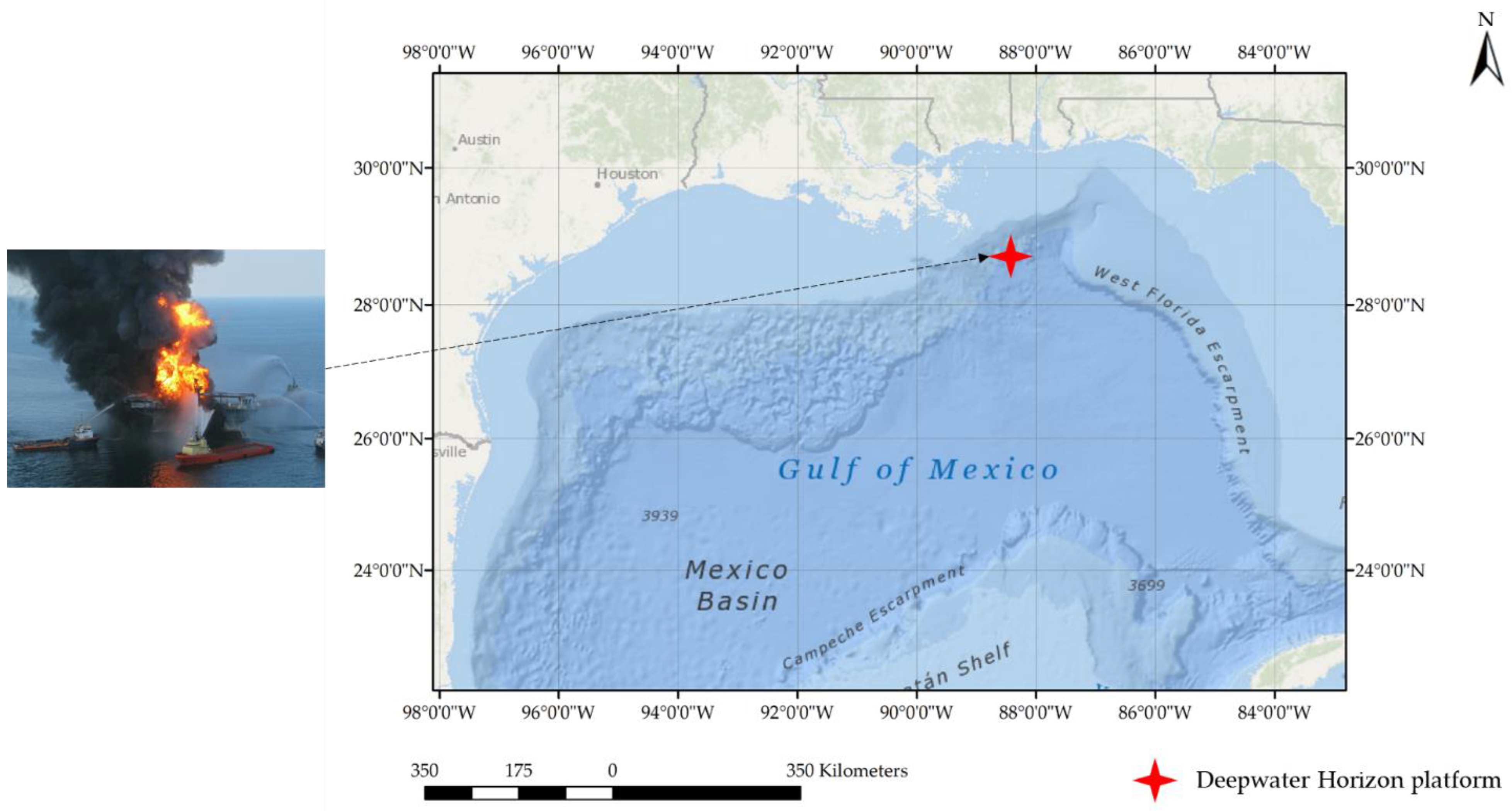
2.1. Study Area

The Deepwater Horizon (DWH) oil spill, resulting from a unpredictable explosion in the Gulf of Mexico in the Macondo seafloor well (28°44′17″N, 88°21′58″W, see Figure 1) operated by the British Petroleum (BP) Public Limited Company, lasted from 20 April 2010 to 19 September 2010 [63,64]. It turned out to be the largest oil spill event in history, with the total volume of leaked petroleum estimated to be 4.9 Mbbl (780,000 m3) with an uncertainty of ±10% [65]. The remote sensing technique served as a quick response to the BP DWH oil spill disaster emergency, and recorded mass data for real-time monitoring and further scientific research [4,66,67,68]. Due to its continuity and wide extent, the DWH oil spill was chosen to evaluate the potential of optical polarization remote sensing for oil spill detection.

2.2. Polarization Satellite Data

Three POLarization and Directionality of the Earth’s Reflectances (POLDER) instruments had been launched to collect optical polarization remote sensing data (see Table 1). The POLDER-1 was selected to fly on the Japanese ADEOS-1 satellite to collect polarized and directional radiance and provide scientific data for climate and global change research from November 1996 to June 1997 [69]. The POLDER-2 was selected to fly on the Japanese ADEOS-2 satellite and provided useful data from April 2003 to October 2003 [70,71]. Unfortunately, the lifetime of the above two platforms was limited to less than a year on account of a failure with the solar panel. The POLDER-3 (which is also named POLDER/PARASOL) was selected to fly on the French PARASOL microsatellite and the PARASOL mission continued to operate from December 2004 to December 2013, exceeding its planned design life by more than 5 years [72,73].
POLDER/PARASOL provides available data on the Gulf of Mexico because the on-orbit duration time of POLDER/PARASOL completely covers the DWH oil spill event. The spectral band characteristics for POLDER/PARASOL are listed in Table 2. The polarization band of 443 nm (443P), polarization band of 670 nm (670P), polarization band of 865 nm (865P), non-polarization band of 443 nm (443NP), non-polarization band of 670 nm (670NP) and non-polarization band of 865 nm (865NP) are used in our comparison experiment to explore the potential of optical polarization remote sensing for oil spill detection.
A full resolution reference grid centered on the Greenwich meridian is used for POLDER/PARASOL L1B products, which is based on the sinusoidal pseudocylindrical equal-area projection (Sanson–Flamsteed projection). The Earth is projected into a 3240 × 6480 raster, which is shown in Figure 2.
The following Equations (1) and (2) describe the relationship between the latitude lat and longitude lon of a given pixel and the coordinates (x, y) in the reference grid:
l a t = 90 x 0.5 18
l o n = 180 NINT [ 3240 cos ( l a t ) ] ( y 3240.5 )
where NINT refers to the nearest integer. In Figure 2, x is in the range of 1 to 3240 from top to bottom and y is in the range of 1 to 6480 from left to right.
In polarization optics, the polarization characteristics are usually described by using the four Stokes parameters: I, Q, U and V [74,75]. The first parameter I describes the total density of the light, the second parameter Q describes the amount of linear horizontal or vertical polarization, the third parameter U describes the amount of linear +45° or −45° polarization and the fourth parameter V describes the amount of right or left circular polarization contained within the beam [76]. The reflection of sunlight by a natural surface generates little elliptic polarization, therefore the fourth Stokes parameter V is not considered because it is relatively small compared to the other three parameters [77]. For POLDER/PARASOL, a polarizer in which an axe is turned by steps of 60° is added to the filters in order to measure the Stokes parameters I, Q and U. The three polarization measurements (0°, 60° and 120°) are successive and there is a 0.3 s time interval between each polarizer rotation, which has been quasi compensated by a three-wedge prism.
The L1B products provide the second parameter Q and the third parameter U. Equations (3)–(5) yield the Stokes parameters that refer to the measured flux density F with three angles: 0°, 60° and 120° [78].
I = 2 3 ( F 0 ° + F 60 ° + F 120 ° )
Q = 4 3 ( 2 F 0 ° F 60 ° F 120 ° )
U = 2 3 3 ( F 120 ° F 60 ° )
The degree of polarization (DoP) is a quantity used to describe the portion of an electromagnetic wave which is polarized, and the phase angle of polarization (AoP, also known as Brewster’s angle) is an angle of incidence at which light with a particular polarization is perfectly transmitted through a transparent dielectric surface, with no reflection [57]. By using the basic polarization information (I, Q and U), the degree of polarization and the phase angle of polarization can be calculated with Equations (6) and (7):
DoP = Q 2 + U 2 I
AoP = 1 2 ARCTAN 2 ( U Q )
where the four-quadrant arctangent operator ARCTAN2(x, y) is defined in Equation (8) [79]:
ARCTAN 2 ( x , y ) = { arctan ( y x ) x > 0 arctan ( y x ) + π y 0 , x < 0 arctan ( y x ) π y < 0 , x < 0 + π 2 y > 0 , x = 0 π 2 y > 0 , x = 0 undefined y = 0 , x = 0
Besides the Stokes parameters, the L1B products also provide the observation geometry information (sun azimuth angle φs, sun zenith angle θs, view azimuth angle φv and view zenith angle θv) when the polarization images are taken. Equation (9) yields the relative azimuth angle φr referring to φs and φv. Equation (10) yields the incidence angle αi referring to θs, θv and φr. Equation (11) yields the angle θm (the angle between the viewing direction and the direction of mirror reflection) referring to θs, θv and φr. Equation (12) yields the scattering angle Θ referring to αi.
φ r = φ s φ v
cos ( 2 α i ) = cos ( θ s ) cos ( θ v ) + sin ( θ s ) sin ( θ v ) cos ( φ r )
cos ( θ m ) = cos ( θ s ) cos ( θ v ) sin ( θ s ) sin ( θ v ) cos ( φ r )
Θ = π 2 α i
According to the Fresnel equation, when light strikes the interface between a medium with refractive index n1 (for instance, atmosphere) and a medium with refractive index n2 (for instance, oil spill), both reflection and refraction of the light are polarized. Equation (13) yields the refraction angle αt referring to αi, and Equation (14) yields the Fresnel function Fp referring to αi and αt.
n 1 sin ( α i ) = n 2 sin ( α t )
F p = 1 2 ( sin 2 ( α t α i ) sin 2 ( α t + α i ) tan 2 ( α t α i ) tan 2 ( α t + α i ) )

2.3. Validation Data

The Satellite Derived Surface Oil Analysis Products-Deepwater Horizon (SDSOAPs-DH) were taken as the validation data (https://www.ssd.noaa.gov/PS/MPS/deepwater.html, accessed on 6 April 2022), which were collected from the National Oceanic and Atmospheric Administration (NOAA) in the framework of the National Environmental Satellite, Data and Information Service (NESDIS). SDSOAPs-DH were produced by Satellite Analysis Branch (SAB) analysts within the NOAA/NESDIS office. SAB analysts integrated multi-source data: synthetic aperture radar (SAR), high resolution visible imagery taken by an unmanned aerial vehicle (UAV) and ancillary reanalyzed data including ocean current information and wind information [80]. SDSOAPs-DH were calibrated with in situ observation results and had passed through a high standard quality control process.
Therefore, SDSOAPs-DH serve as adequate validation data of POLDER/PARASOL, given that the spatial resolution of POLDER/PARASOL is close to 6 km in nadir, which turns out to be relatively coarse. A total of 84 shapefiles from 17 May 2010 to 25 August 2010 were downloaded from the SDSOAPs-DH dataset, which were vector files applicable for ArcGIS demonstration. After eliminating 15 shapefiles in which the oil spill area was too small to recognize, 70 validation data were chosen to match with satellite data.
Since polarization satellite data are raster data and validation data are vector shapefiles, a resampling process of the validation data was performed in advance. All the shapefiles were first converted to rasters by using ArcMap 10.7.1 Conversion Tools, and the cell size was set to be 2 km. It can be guaranteed that each cell in a Sanson–Flamsteed raster is in the center of 3 × 3 cells of the 2 km validation raster data, and the 2 km validation raster data are resampled to Sanson–Flamsteed raster data via the average calculation and rounding operation of 3 × 3 cells. The pre-processed binary time-series images utilized for validation are shown in Figure 3 (time-series images are taken from the same scene at different times).

2.4. Random Forest Classifier

Previous studies have used random forest classifiers to detect oil spill [81,82,83], and most of them are related to SAR images. Since optical polarization shares a similarity with SAR, a random forest classifier adjusted for optical polarization application was trained to distinguish the oil spill pixels (labelled as 1) from sea water pixels (labelled as 0) in our experiment. In the process of random forest classification, a single random forest is a meta estimator that fits a number of decision tree classifiers on various sub-samples of the dataset and uses averaging to improve the predictive accuracy and control over-fitting. In our study, a random forest classifier was carried out by using “sklearn.ensemble.RandomForestClassifier” in the scikit-learn 1.0.2 package.
Since the data quality for angles 1, 14, 15 and 16 was not acceptable (there exists many pixels filled with ±32,767, which refers to missing data or poor quality), only 12 angles were used for model training. In order to solve Q1, Q2, Q3, Q4a and Q4b, 24 different feature combinations were organized (the specific descriptions of all combinations are listed in Table 3). Combination Opt refers to the pure optical remote sensing data, and it contains only radiance L in three bands (490 nm, 670 nm and 865 nm). It is noted that combination Opt is the basic combination which includes no auxiliary information concerning polarization characteristics and observation geometry. Combination rawPol refers to the polarization raw data that is gained by rotating the polarizer and then measuring the flux density F with three angles: 0°, 60° and 120°. Combination rawPol is the unprocessed polarization data and it contains the original polarization information acquired by the POLDER/PARASOL. Combination IQUV refers to the Stokes parameters which can be calculated by Equations (3)–(5). Combination DoP refers to the degree of polarization which can be calculated by Equation (6). Combination AoP refers to the phase angle of polarization which can be calculated by Equation (7). Combination DoPAoP is the coupling of combinations DoP and AoP, which allows to characterize polarization information in two different aspects (combination DoP focuses on the level of polarization versus conventional optics, and combination AoP focuses on the orientation of polarization eclipse). The difference between combinations XXX and XXX_s (XXX = Opt, rawPol, IQUV, DoP, AoP and DoPAoP) lies on the expression of observation geometry, and it was designed to study Q2. The observation geometry for combination XXX is expressed with sun zenith angle θs, view zenith angle θv and relative azimuth angle φr, whereas the observation geometry for combination XXX_s is expressed with scattering angle Θ. Combinations Opt, rawPol, IQUV, DoP, AoP, DoPAoP, Opt_s, rawPol_s, IQUV_s, DoP_s, AoP_s and DoPAoP_s were used to explore the potential of optical polarization remote sensing (Q1), and combinations rawPol, IQUV, DoP, AoP, DoPAoP, rawPol_s, IQUV_s, DoP_s, AoP_s and DoPAoP_s were used to decide the best form of polarization characteristics (Q3). For the above combinations, the data of 12 angles were stacked to generate the trained features, but the combinations DoPAoP_s_anglex (x = 2, 3, …, 13) only contain data of a single angle which were designed to study Q4a and Q4b.
A 10-fold cross-validation was utilized to assess the performance of our trained model with different expressions of polarization characteristics (the code of cross-validation was programmed in Python 3.8, and the single floating-point datatype “float” was used for the assessment, which led to a minor difference in the final result). In the 10-fold cross-validation strategy, all the labelled data were divided into 10 equivalent groups after the POLDER/PARASOL satellite data and SDSOAPs-DH validation data were matched and stacked. Then, 9 groups were taken as the training data and 1 group was used for the model assessment. This procedure ran 10 times until every single group was chosen for the random forest classifier validation. The overall accuracy, recall (also called the true positive rate), precision (also called the positive predictive value) and F1 score can be calculated with Equations (15)–(18):
accuracy = t p + t n t p + t n + f p + f n
recall = t p t p + f n
precision = t p t p + f p
F 1 = 2 p p v 1 + t p r 1
where tp refers to true positive pixels, tn refers to true negative pixels, fp refers to false positive pixels and fn refers to false negative pixels.

3. Results

Our study focused on several key questions (Q1, Q2, Q3 and Q4), which were designed to explore the potential of optical polarization remote sensing in oil spill detection (specifically, what kinds of influences would different forms of polarization information introduce in the existing random forest classifier frame). The results of the random forest classifier are outlined in the following paragraphs.
The results for combinations Opt, rawPol, IQUV, DoP, AoP, DoPAoP, Opt_s, rawPol_s, IQUV_s, DoP_s, AoP_s and DoPAoP_s are listed in Table 4, which help to answer Q1, Q2 and Q3.

3.1. Q1. To What Extent Do Polarization Characteristics Help in Optical Remote Sensing for Oil Spill Detection?

When the observation geometry was expressed with sun zenith angle θs, view zenith angle θv and relative azimuth angle φr, combinations rawPol, IQUV and DoPAoP outperformed combination Opt in the four evaluation indicators, especially in precision and F1. The average increase of accuracy and recall was only +0.59% and +1.70%, respectively, which was not conspicuous. However, the average increase of precision was +6.09% with the maximum reach up to +6.92%, and the average increase of the F1 score was +3.26% with the maximum reach up to +4.72%, suggesting that polarization characteristics help optical remote sensing to a large extent from the prospect of oil spill detection (recall and precision evaluate the model in two different aspects: for recall, the denominator of Equation (16) is tp + fn, which means all the right predictions are taken into account, focusing on the classification including oil spill and sea water, and thus it shows a label-priority tendency, which means the model is apt to give every pixel a right label; for precision, the denominator of Equation (17) is tp + fp, which means the both the right or wrong oil spill predictions are taken into account, paying more attention to the detection of oil spill regardless of sea water, and thus it shows a task-priority tendency, which means the model is apt to complete the task of oil spill detection).
When the observation geometry was expressed with scattering angle Θ, combinations rawPol, IQUV and DoPAoP also outperformed combination Opt in the four evaluation indicators, especially in recall and F1. The average increase of accuracy and precision was only +0.43% and +0.89%, respectively. However, the average increase of recall was +3.96% with the maximum reach up to 5.09%, and the average increase of the F1 score was +2.75% with the maximum reach up to +3.98%, suggesting that polarization characteristics help optical remote sensing to a large extent from the prospect of classification between oil spill and sea water.
In summary, for two ways of expressing observation geometry, combinations with polarization information outperformed the combinations with only optical information in four evaluation indicators. The accuracy rise was not obvious with an average increase of +0.51%, but still reflects an acceptable improvement in our trained models considering that the accuracy has already exceeded 95%, which makes the further numeric promotion in accuracy difficult. The rise of recall and precision was much higher than that of accuracy, but not stable. The average increase of recall and precision was +2.83% and +3.49%, respectively, but the maximum increase could reach two to three times the average value, suggesting that the classifier models established with the aid of polarization information have no clear tendency between label-priority and task-priority strategies. The increase of F1 was obvious and stable, with an average of +3.01% and a maximum of +4.72%, suggesting that polarization characteristics provide considerable help in optical remote sensing for oil spill detection with recall and precision considered equally.

3.2. Q2. How Do Different Ways of Expressing Observation Geometry Influence the Result of Oil Spill Detection?

Comparing six combination pairs (Opt and Opt_s, rawPol and rawPol _s, IQUV and IQUV_s, DoP and DoP_s, AoP and AoP_s, and DoPAoP and DoPAoP_s), two advantages of using the scattering angle Θ to simplify observation geometry were discovered instead of using the traditional expression (sun zenith angle θs, view zenith angle θv and relative azimuth angle φr).
The first advantage lies in the acceleration of training speed. For the scattering angle expression, the training time was −12.04% less than that of the traditional expression, which can be ascribed to the decrease of two dimensions in feature vectors.
The second advantage lies in the improvement of model performance. The average increase of accuracy was +1.20%, which was the lowest among the four indicators. However, this increase still counts, for the accuracy of oil spill detection was already beyond 95% and a breakthrough of 98% is regarded as a process of quantitative alteration to qualitative alteration. The average rise of recall and precision was +12.43% and +1.10%, respectively, indicating that the scattering angle expression contributes much more in label-priority strategy than task-priority strategy. The F1 score serves as the most comprehensive indicator for random forest classifier ability assessment. A mean rise of +8.44% and maximum rise of +9.23% in the F1 score showed a significant improvement of model ability when applying the scatter angle expression.
In summary, using the scattering angle Θ to describe observation geometry, instead of using the sun zenith angle θs, view zenith angle θv and relative azimuth angle φr, has a great positive influence on the increase of model performance and the decrease of training time.

3.3. Q3. Which Combination of Polarization Features Performs Better in Oil Spill Detection?

In the comparisons, five ways of polarization feature description were taken into account, including directional polarization data (combinations rawPol and rawPol_s), Stokes parameters (combinations IQUV and IQUV_s), degree of polarization (combinations DoP and DoP_s), phase angle of polarization (combinations AoP and AoP_s) and degree and phase angle of polarization (combinations DoPAoP and DoPAoP_s).
When the observation geometry was expressed with the sun zenith angle θs, view zenith angle θv and relative azimuth angle φr, combinations rawPol, IQUV and DoPAoP outperformed combination Opt, but combinations DoP and AoP resulted in poor performance (the possible reason for poor performance in combinations DoP and AoP is discussed in Section 4.2). Combination DoPAoP was the best combination with an overwhelming gap in four indicators (+0.80% in accuracy, +3.39% in recall, +6.92% in precision and +4.72% in the F1 score).
When the observation geometry was expressed with the scattering angle Θ, the results were similar and combination DoPAoP_s was also the best combination regarding the numerical advantage of four indicators (+0.64% in accuracy, +5.09% in recall, +2.22% in precision and +3.98% in the F1 score).
In summary, combinations DoPAoP and DoPAoP_s performed the best in oil spill detection, indicating that combining the degree of polarization and phase angle of polarization simultaneously is the best way to detect oil spill in our study.
The results for combinations DoPAoP_s, DoPAoP_s_angle2, DoPAoP_s_angle3, DoPAoP_s_angle4, DoPAoP_s_angle5, DoPAoP_s_angle6, DoPAoP_s_angle7, DoPAoP_s_angle8, DoPAoP_s_angle9, DoPAoP_s_angle10, DoPAoP_s_angle11, DoPAoP_s_angle12 and DoPAoP_s_angle13 are listed in Table 5, which help to answer Q4.

3.4. Q4. Which Single-Angle Polarization Data Provide Better Oil Spill Detection Performance?

Comparing model performance of single-angle combinations DoPAoP_s_anglex (x = 2, 3, …, 13) with multiple-angle combination DoPAoP_s, it can be concluded that most single-angle combinations exert a sharp decrease on model performance except for angle8 and angle9. The average performance degradation in four indicators for anglex (x = 2, 3, …, 7, 10, …, 13) observation was −4.40% in accuracy, −41.36% in recall, −12.54% in precision and −35.30% in the F1 score, which is apparently not suitable for application, indicating that the information carried in these twelve angles is barely useful for oil spill detection. The average performance degradation in four indicators for angle8 and angle9 was acceptable (−1.03% in accuracy, −5.93% in recall, −6.22% in precision and −6.12% in the F1 score), proving that angle8 and angle9 polarization data carry the most useful information which is beneficial for oil spill detection (the possible reason for angle sensibility is discussed in Section 4.3). In summary, single-angle polarization data of angle8 and angle9 provide better oil spill detection performance.

4. Discussion

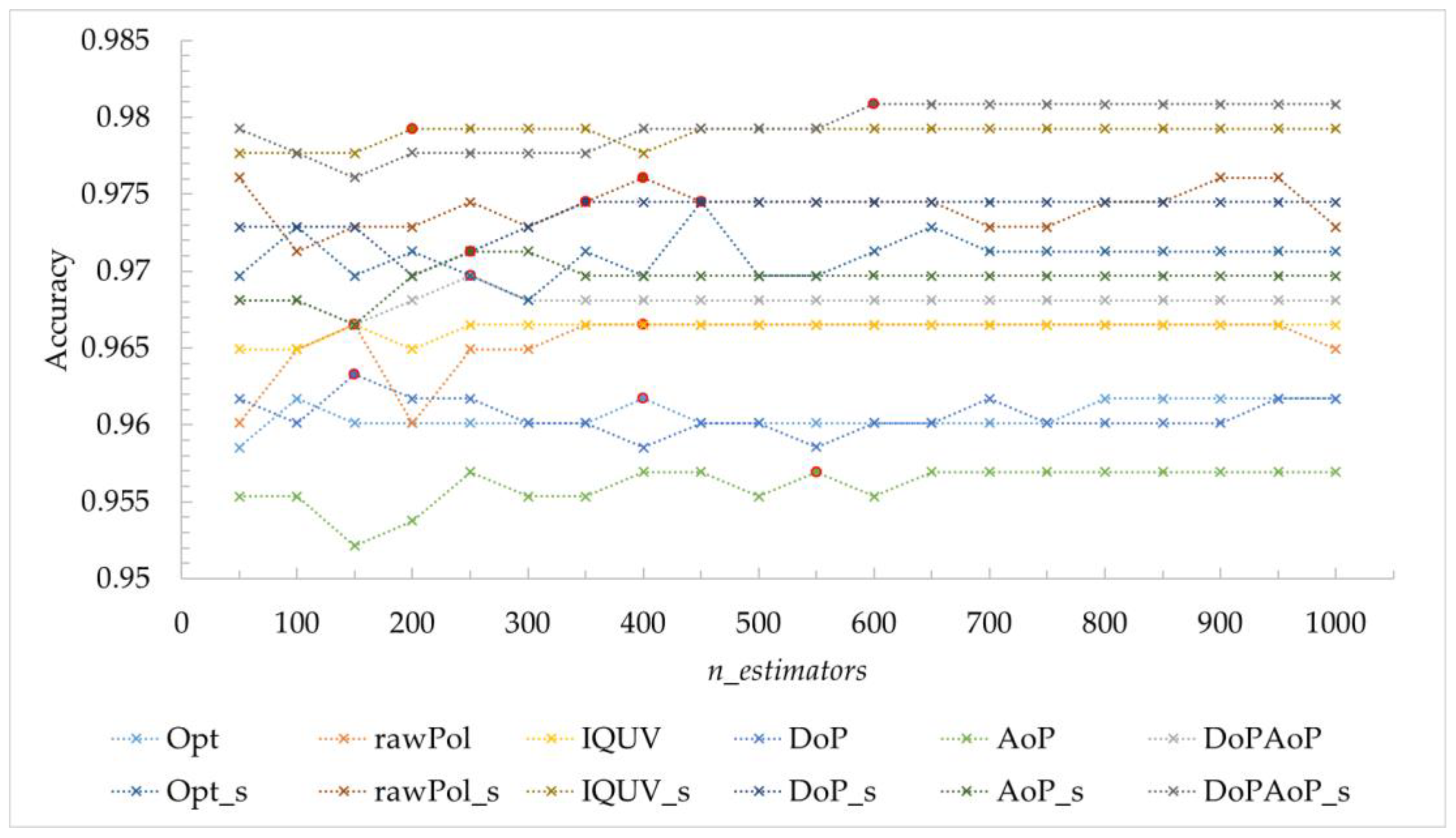
4.1. Determining Random Forest Classifier Parameters

For the random forest classifier, there are four major influencing parameters, including criterion, max_depth, max_feature and n_estimators. Adjusting algorithm parameters helped to obtain a better performance in oil spill detection. criterion was fixed to be “Gini” for all the models trained in our experiment, which means Gini impurity was chosen to measure the quality of each split. max_depth was set to be “None”; therefore, before all the tree leaves were pure or included samples which were under the minimum, every node was continuously expanded. max_feature was fixed to be “Sqrt” for all our models, which means max_feature = sqrt(n_features). The specific definitions of terms related to the random forest classifier are shown in Appendix A Table A1.
n_estimators referred to the number of trees in the forest, and the adjustment of this parameter enhanced the model performance and training speed. For different combinations tested and trained in our experiment, the optimal n_estimators was unique. The accuracy and F1 score were calculated to select the optimal n_estimators (as mentioned above, the F1 score is the harmonic average of recall and precision, and it can stand for these two indicators to a certain extent). The criteria for determining the optimal n_estimators are: (1) the lowest n_estimators which maximizes the F1 score and accuracy; and (2) if the maximum of the F1 score and accuracy cannot be achieved at the same time, the F1 score will be taken as the priority indicator. n_estimators ranging from 50–1000 with an interval of 50 trees were utilized to select the optimal parameter. In Figure 4 and Figure 5, the regular values are marked with an “×” and the optimal values are marked with a red-edged “○” in order to highlight the final choice.
The purpose of random forest classification is to determine the class by the input features (in our experiment, the final purpose was to label whether the pixel belonged to oil spill or sea water). On the other hand, the purpose of random forest regression is to predict a specific value. This difference in final purpose leads to the difference in result validation and parameter adjusting. For random forest classification, a little bias before the internal decision-making process could not change the output class, and thus imposes no effect on the quantitative validation value, which is the reason why the curves shown in Figure 4 and Figure 5 are gradually flattened to be completely unchanged as the models grow stable. On the contrary, for random forest regression, the curves will finally fluctuate within a narrow range due to the direct influence of the tiny prediction error.

4.2. Coupling between Degree of Polarization and Phase Angle of Polarization

In Q3, combinations DoPAoP and DoPAoP_s performed the best in oil spill detection, indicating that combining the degree of polarization and phase angle of polarization simultaneously is the best way to detect oil spill in our experiment. However, when the degree of polarization and phase angle of polarization were applied, the performance was even worse than the optical baseline combination. Combinations DoP and AoP suffered from an average −1.56% decrease and maximum −3.39% decrease in four indicators compared to Opt, and combinations DoP_s and AoP_s suffered from an average −0.71% decrease and maximum −3.58% decrease in four indicators compared to Opt_s. Despite that the decreasing amplitude was not sharp, the decreasing trend cannot be ignored compared with the best performance earned by the combinations DoPAoP and DoPAoP_s, which are the coupling of combinations DoP and AoP.
This may result in the coupling mechanism between the degree of polarization and phase angle of polarization. When these two characteristics are used separately, the degree of polarization refers to the ratio of the polarized component to the total light intensity, which is the macroscopic expression of the polarization level, and the phase angle of polarization refers to the orientation of the polarization ellipse, which is the detailed expression in the projection plane. Therefore, the degree of polarization and phase angle of polarization cannot conclude polarization separately due to each’s single-sided perspective. As a result, coupling between the degree of polarization and phase angle of polarization receives a better effect than directional polarization combinations rawPol and rawPol_s and Stokes parameter combinations IQUV and IQUV_s.

4.3. Sensibility Analysis of Observation Geometry

In regard to Q4, single-angle polarization data of angle8 and angle9 provided a better oil spill detection performance. The performance of single-angle observation is determined by angle θm (the angle between the viewing direction and the direction of mirror reflection, see Equation (11)). Angle θm indicates the strength of sun glint, and the smaller the value of θm, the stronger the sun glint [84]. Previous works [61,62] have demonstrated that polarization information helps to identify oil spill when the observed area is under sun glint (when −20° < θm < 20°, the polarization model agrees well). In our experiment, the average θm for the observation of angle8 and angle9 was −13.74° and 14.63°, respectively, suggesting that angle8 and angle9 refer to strong sun glint observations and cope with the polarization reflection model well. The reason is that the observation geometry of strong sun glint corresponds with the agreement of the polarization model and the ignorable atmospheric polarization effects, which helps to enhance the effectiveness of polarization information. In addition, the change of θm of anglex (x = 2, 3, …, 13) showed an obvious trend that θm gradually approached 0° before angle8 and then kept away from 0° after angle9, which is in accordance with the trend in Table 5.

4.4. Limitations and Future Work

In our experiment, there were three major limitations.
The first limitation lies in the complex interaction in a coupled ocean–atmosphere system, which could lead to large differences between the water-leaving polarization status and top-of-atmosphere polarization status. In order to detect the oil spill, an accurate estimate of water-leaving polarization status is required. In our experiment, only data with cloud_flag = 0 (it suggests that there is almost no cloud and influence of atmosphere could be weakened to some extent) were chosen to reduce the influence of atmosphere. Our results verify the conclusion in [62] that the atmospheric polarization effects can be neglected in angle8 and angle9; thus, the oil spill detection results are trustworthy. However, in the future, if accurate polarization correction of anglex (x = 2, 3, …, 7, 10, …, 13) can be conducted by a vector radiative transfer model in a coupled ocean–atmosphere system, then the available polarization information would largely increase, as would the results in the promotion of model performance for oil spill detection.
The second limitation lies in the mixed pixel problem. Since the spatial resolution of POLDER/PARASOL is coarse (approximately 6 km in nadir), there would be many pixels stepping over the border between oil spill and sea water, which leads to difficulty in classification (because these mixed pixels appear to be compound characteristics). In the future, when a new satellite armed with a high resolution polarization sensor is launched (future missions concerning optical polarization observation are shown in Appendix A Table A2) and the thickness of oil spill could be measured at the same time, a new polarization feature should be established to extract polarization information and the retrieval of oil spill thickness may become possible.
The third limitation lies in the baseline method used in our experiment. A pixel-based random forest classifier was chosen for its simplicity and practicability because the major purpose of our work was to explore the potential of polarization remote sensing in oil spill detection. In the future, some object-based classifiers, which could extract topological information between adjacent pixels, could be utilized to obtain a better oil spill detection performance.

5. Conclusions

In our study, POLDER/PARASOL polarization images and SDSOAPs-DH data were used to conduct the training and validation. A total of 24 feature combinations (including optical data, raw polarization data, Stokes parameter data, degree of polarization data, phase angle of polarization data, coupling degree and phase angle of polarization data and single-angle data) were tested using a random forest classifier to solve four questions aimed at exploring the potential of optical polarization remote sensing for oil spill detection. The results show that: (1) combinations with polarization information embody great advantages on model performance over accuracy, recall, precision and the F1 score; (2) using a scattering angle to express observation geometry helps to detect oil spill, improving model performance and reducing training time; (3) coupling between the degree of polarization and phase angle of polarization provides the best performance for oil spill detection; and (4) angle8 and angle9 offer the most major, useful information out of the 13 angles.
This paper confirms the potential of optical polarization remote sensing for oil spill detection and depicts a scientific roadmap for future development through detailed discussion. The methods and conclusions mentioned in our experiment can be applied to other oil spill events if the spatial resolution of the optical polarization sensor is consistent with the scale of oil spill. In the future, the application of optical polarization remote sensing on oil spill research would be beneficial for the improvement of detection ability, the saving of observation costs and the possibility of oil spill thickness retrieval.

Author Contributions

Conceptualization, Z.Z., F.Z., L.Y., X.J. and J.D.; methodology, Z.Z.; software, Z.Z.; validation, Z.Z., K.J. and K.S.; formal analysis, Z.Z.; writing—original draft preparation, Z.Z.; writing—review and editing, F.Z., L.Y., X.J. and J.D.; visualization, Z.Z., K.J. and K.S.; funding acquisition, F.Z., L.Y., X.J. and J.D. All authors have read and agreed to the published version of the manuscript.

Funding

This research was funded by the National Key R&D Program of China (grant number 2017YFB0503004) and Key R&D Program of Hebei Province (grant number 21373301D).

Data Availability Statement

POLDER/PARASOL L1B products (https://www.icare.univ-lille.fr/data-access/data-archive-access/?dir=PARASOL/L1_B-HDF/2010/, accessed on 6 April 2022) and Satellite Derived Surface Oil Analysis Products-Deepwater Horizon (https://www.ssd.noaa.gov/PS/MPS/deepwater.html, accessed on 6 April 2022).

Conflicts of Interest

The authors declare no conflict of interest.

Appendix A

Table A1. The definitions of terms related to the random forest classifier (the terms in italic font refer to the input parameters for the random forest classifier).
TermDefinitionFormula
classification treeClassification trees are tree models where the target variable can take a discrete set of values./
leafIn classification trees, leaves refer to the class labels./
branchIn classification trees, branches refer to the conjunctions of features./
nodeIn classification trees, nodes refer to the branch points./
n_featuresThe number of features during fit./
max_featureThe maximum of features when looking for the best split.max_feature = sqrt(n_features)
or max_feature = log2(n_features)
criterionThe function to measure the quality of a split. Gini impurity is the recommended function./
Gini impurityA function that determines how well a decision tree is split. (D refers to the dataset, and pi refers to the probability of samples belonging to class i at a given node.) Gini ( D ) = 1 i = 1 k p i 2
max_depthThe maximum depth of the tree./
n_estimatorsThe number of trees in the forest./
Table A2. Comparisons between future missions concerning optical polarization observation [85,86,87,88].
SensorSpatial ResolutionSpectral RangeScheduled Launch Time
3MI/EPS-SG4 km410 nm, 443 nm, 490 nm, 555 nm, 670 nm, 865 v, 1370 nm, 1650 nm, 2130 nm2022–2023
SPEXone/PACE2.5 km385–770 nm in 2–4 nm steps2023
HARP2/PACE3 km440 nm, 550 nm, 670 nm, 870 nm2023
PolCube0.39 km × 0.31 km410 nm, 555 nm, 670 nm, 865 nm2023
ScanPol/Aerosol-UA0.2–0.5 km370 nm, 410 nm, 555 nm, 865 nm, 1378 nm, 1610 nm2025
MSIP/Aerosol-UA0.2–0.5 km410 nm, 555 nm, 865 nm2025

References

  1. Perrons, R.K. Assessing the damage caused by Deepwater Horizon: Not just another Exxon Valdez. Mar. Pollut. Bull. 2013, 71, 20–22. [Google Scholar] [CrossRef] [PubMed]
  2. Wang, J.; Shen, Y. Development of an integrated model system to simulate transport and fate of oil spills in seas. Sci. China Technol. Sci. 2010, 53, 2423–2434. [Google Scholar] [CrossRef]
  3. Castanedo, S.; Juanes, J.; Medina, R.; Puente, A.; Fernandez, F.; Olabarrieta, M.; Pombo, C. Oil spill vulnerability assessment integrating physical, biological and socio-economical aspects: Application to the Cantabrian coast (Bay of Biscay, Spain). J. Environ. Manag. 2009, 91, 149–159. [Google Scholar] [CrossRef] [PubMed]
  4. Leifer, I.; Lehr, W.J.; Simecek-Beatty, D.; Bradley, E.; Clark, R.; Dennison, P.; Hu, Y.; Matheson, S.; Jones, C.E.; Holt, B. State of the art satellite and airborne marine oil spill remote sensing: Application to the BP Deepwater Horizon oil spill. Remote Sens. Environ. 2012, 124, 185–209. [Google Scholar] [CrossRef] [Green Version]
  5. Fingas, M.; Brown, C.E. Oil spill remote sensing: A forensics approach. In Standard Handbook Oil Spill Environmental Forensics; Elsevier: Amsterdam, The Netherlands, 2016; pp. 961–981. [Google Scholar]
  6. Fingas, M.; Brown, C.E. A review of oil spill remote sensing. Sensors 2018, 18, 91. [Google Scholar] [CrossRef] [PubMed] [Green Version]
  7. Fingas, M.; Brown, C. Review of oil spill remote sensing. Mar. Pollut. Bull. 2014, 83, 9–23. [Google Scholar] [CrossRef] [Green Version]
  8. Brekke, C.; Solberg, A.H. Oil spill detection by satellite remote sensing. Remote Sens. Environ. 2005, 95, 1–13. [Google Scholar] [CrossRef]
  9. Suo, Z.; Lu, Y.; Liu, J.; Ding, J.; Yin, D.; Xu, F.; Jiao, J. Ultraviolet remote sensing of marine oil spills: A new approach of Haiyang-1C satellite. Opt. Express 2021, 29, 13486–13495. [Google Scholar] [CrossRef]
  10. Li, Y.; Li, B.; Lin, G.; Huang, Y.; Yang, D.; Ma, Y. Ultraviolet Radiation Characteristic of Oil Spills on Sea Surface. Acta Opt. Sin. 2020, 40, 0801001. [Google Scholar]
  11. Cong, H. Characteristics of UV Reflection Spectra of Oil Spill Based on Bidirectional Reflectance Distribution Function. Acta Photonica Sin. 2017, 46, 1012002. [Google Scholar] [CrossRef]
  12. Fang, S.; Huang, X.; Yin, D.; Xu, C.; Feng, X.; Feng, Q. Research on the ultraviolet reflectivity characteristic of simulative targets of oil spill on the ocean. Spectrosc. Spectr. Anal. 2010, 30, 738–742. [Google Scholar]
  13. Guo, G.; Liu, B.; Liu, C. Thermal infrared spectral characteristics of bunker fuel oil to determine oil-film thickness and API. J. Mar. Sci. Eng. 2020, 8, 135. [Google Scholar] [CrossRef] [Green Version]
  14. Zhou, Y.; Jiang, L.; Lu, Y.; Zhan, W.; Mao, Z.; Qian, W.; Liu, Y. Thermal infrared contrast between different types of oil slicks on top of water bodies. IEEE Geosci. Remote Sens. Lett. 2017, 14, 1042–1045. [Google Scholar] [CrossRef]
  15. Lu, Y.; Zhan, W.; Hu, C. Detecting and quantifying oil slick thickness by thermal remote sensing: A ground-based experiment. Remote Sens. Environ. 2016, 181, 207–217. [Google Scholar] [CrossRef]
  16. Xing, Q.; Li, L.; Lou, M.; Bing, L.; Zhao, R.; Li, Z. Observation of oil spills through landsat thermal infrared imagery: A case of deepwater horizon. Aquat. Procedia 2015, 3, 151–156. [Google Scholar] [CrossRef]
  17. Yang, J.; Ma, Y.; Hu, Y.; Jiang, Z.; Zhang, J.; Wan, J.; Li, Z. Decision Fusion of Deep Learning and Shallow Learning for Marine Oil Spill Detection. Remote Sens. 2022, 14, 666. [Google Scholar] [CrossRef]
  18. Duan, P.; Xie, Z.; Kang, X.; Li, S. Self-supervised learning-based oil spill detection of hyperspectral images. Sci. China Technol. Sci. 2022, 65, 793–801. [Google Scholar] [CrossRef]
  19. Caillault, K.; Roupioz, L.; Viallefont-Robinet, F. Modelling of the optical signature of oil slicks at sea for the analysis of multi-and hyperspectral VNIR-SWIR images. Opt. Express 2021, 29, 18224–18242. [Google Scholar] [CrossRef]
  20. Khanna, S.; Santos, M.J.; Ustin, S.L.; Shapiro, K.; Haverkamp, P.J.; Lay, M. Comparing the potential of multispectral and hyperspectral data for monitoring oil spill impact. Sensors 2018, 18, 558. [Google Scholar] [CrossRef] [Green Version]
  21. Moon, J.; Jung, M. Geometrical Properties of Spilled Oil on Seawater Detected Using a LiDAR Sensor. J. Sens. 2020, 2020, 5609168. [Google Scholar] [CrossRef]
  22. Jing, L.; Ying, C.; Shuang, L.; Zhaoxin, W.; Kun, Y. Design of Lidar System Based on Marine Oil Spill Monitoring. In Proceedings of the E3S Web of Conferences, Jilin, China, 20–22 March 2020; p. 03052. [Google Scholar] [CrossRef]
  23. Alaruri, S.D. Multiwavelength laser induced fluorescence (LIF) LIDAR system for remote detection and identification of oil spills. Optik 2019, 181, 239–245. [Google Scholar] [CrossRef]
  24. Raimondi, V.; Palombi, L.; Lognoli, D.; Masini, A.; Simeone, E. Experimental tests and radiometric calculations for the feasibility of fluorescence LIDAR-based discrimination of oil spills from UAV. Int. J. Appl. Earth Obs. Geoinf. 2017, 61, 46–54. [Google Scholar] [CrossRef]
  25. Jiao, J.; Lu, Y.; Liu, Y. Optical quantification of oil emulsions in multi-band coarse-resolution imagery using a lab-derived HSV model. Mar. Pollut. Bull. 2022, 178, 113640. [Google Scholar] [CrossRef] [PubMed]
  26. Seydi, S.T.; Hasanlou, M.; Amani, M.; Huang, W. Oil Spill Detection Based on Multiscale Multidimensional Residual CNN for Optical Remote Sensing Imagery. IEEE J. Sel. Top. Appl. Earth Obs. Remote Sens. 2021, 14, 10941–10952. [Google Scholar] [CrossRef]
  27. Zhao, J.; Temimi, M.; Ghedira, H.; Hu, C. Exploring the potential of optical remote sensing for oil spill detection in shallow coastal waters-a case study in the Arabian Gulf. Opt. Express 2014, 22, 13755–13772. [Google Scholar] [CrossRef]
  28. Lu, Y.; Li, X.; Tian, Q.; Zheng, G.; Sun, S.; Liu, Y.; Yang, Q. Progress in marine oil spill optical remote sensing: Detected targets, spectral response characteristics, and theories. Mar. Geod. 2013, 36, 334–346. [Google Scholar] [CrossRef]
  29. Huang, X.; Zhang, B.; Perrie, W.; Lu, Y.; Wang, C. A novel deep learning method for marine oil spill detection from satellite synthetic aperture radar imagery. Mar. Pollut. Bull. 2022, 179, 113666. [Google Scholar] [CrossRef]
  30. Jafarzadeh, H.; Mahdianpari, M.; Homayouni, S.; Mohammadimanesh, F.; Dabboor, M. Oil spill detection from Synthetic Aperture Radar Earth observations: A meta-analysis and comprehensive review. GIScience Remote Sens. 2021, 58, 1022–1051. [Google Scholar] [CrossRef]
  31. Cai, Y.; Zou, Y.; Liang, C.; Zou, B. Research on polarization of oil spill and detection. Acta Oceanol. Sin. 2016, 35, 84–89. [Google Scholar] [CrossRef]
  32. Cheng, Y.; Li, X.; Xu, Q.; Garcia-Pineda, O.; Andersen, O.B.; Pichel, W.G. SAR observation and model tracking of an oil spill event in coastal waters. Mar. Pollut. Bull. 2011, 62, 350–363. [Google Scholar] [CrossRef]
  33. Ma, X.; Xu, J.; Wu, P.; Kong, P. Oil Spill Detection Based on Deep Convolutional Neural Networks Using Polarimetric Scattering Information From Sentinel-1 SAR Images. IEEE Trans. Geosci. Remote Sens. 2022, 60, 1–13. [Google Scholar] [CrossRef]
  34. Naz, S.; Iqbal, M.F.; Mahmood, I.; Allam, M. Marine oil spill detection using Synthetic Aperture Radar over Indian Ocean. Mar. Pollut. Bull. 2021, 162, 111921. [Google Scholar] [CrossRef] [PubMed]
  35. Guo, H.; Wu, D.; An, J. Discrimination of oil slicks and lookalikes in polarimetric SAR images using CNN. Sensors 2017, 17, 1837. [Google Scholar] [CrossRef] [Green Version]
  36. Chen, G.; Li, Y.; Sun, G.; Zhang, Y. Application of deep networks to oil spill detection using polarimetric synthetic aperture radar images. Appl. Sci. 2017, 7, 968. [Google Scholar] [CrossRef]
  37. Marghany, M. Automatic Mexico gulf oil spill detection from Radarsat-2 SAR satellite data using genetic algorithm. Acta Geophys. 2016, 64, 1916–1941. [Google Scholar] [CrossRef] [Green Version]
  38. King, M.D.; Platnick, S.; Menzel, W.P.; Ackerman, S.A.; Hubanks, P.A. Spatial and temporal distribution of clouds observed by MODIS onboard the Terra and Aqua satellites. IEEE Trans. Geosci. Remote Sens. 2013, 51, 3826–3852. [Google Scholar] [CrossRef]
  39. Hu, C.; Lu, Y.; Sun, S.; Liu, Y. Optical remote sensing of oil spills in the ocean: What is really possible? J. Remote Sens. 2021, 2021, 9141902. [Google Scholar] [CrossRef]
  40. Sun, S.; Hu, C. The challenges of interpreting oil–water spatial and spectral contrasts for the estimation of oil thickness: Examples from satellite and airborne measurements of the deepwater horizon oil spill. IEEE Trans. Geosci. Remote Sens. 2018, 57, 2643–2658. [Google Scholar] [CrossRef]
  41. Lu, Y.; Shi, J.; Hu, C.; Zhang, M.; Sun, S.; Liu, Y. Optical interpretation of oil emulsions in the ocean–Part II: Applications to multi-band coarse-resolution imagery. Remote Sens. Environ. 2020, 242, 111778. [Google Scholar] [CrossRef]
  42. Lu, Y.; Shi, J.; Wen, Y.; Hu, C.; Zhou, Y.; Sun, S.; Zhang, M.; Mao, Z.; Liu, Y. Optical interpretation of oil emulsions in the ocean–Part I: Laboratory measurements and proof-of-concept with AVIRIS observations. Remote Sens. Environ. 2019, 230, 111183. [Google Scholar] [CrossRef]
  43. Clark, R.N.; Swayze, G.A.; Leifer, I.; Livo, K.E.; Kokaly, R.; Hoefen, T.; Lundeen, S.; Eastwood, M.; Green, R.O.; Pearson, N. A method for quantitative mapping of thick oil spills using imaging spectroscopy. US Geol. Surv. Open-File Rep. 2010, 1167, 1–51. [Google Scholar]
  44. Yan, L.; Li, Y.; Chandrasekar, V.; Mortimer, H.; Peltoniemi, J.; Lin, Y. General review of optical polarization remote sensing. Int. J. Remote Sens. 2020, 41, 4853–4864. [Google Scholar] [CrossRef]
  45. Rozanov, V.; Dinter, T.; Rozanov, A.; Wolanin, A.; Bracher, A.; Burrows, J. Radiative transfer modeling through terrestrial atmosphere and ocean accounting for inelastic processes: Software package SCIATRAN. J. Quant. Spectrosc. Radiat. Transf. 2017, 194, 65–85. [Google Scholar] [CrossRef] [Green Version]
  46. Chami, M.; Lafrance, B.; Fougnie, B.; Chowdhary, J.; Harmel, T.; Waquet, F. OSOAA: A vector radiative transfer model of coupled atmosphere-ocean system for a rough sea surface application to the estimates of the directional variations of the water leaving reflectance to better process multi-angular satellite sensors data over the ocean. Opt. Express 2015, 23, 27829–27852. [Google Scholar]
  47. He, X.; Bai, Y.; Zhu, Q.; Gong, F. A vector radiative transfer model of coupled ocean–atmosphere system using matrix-operator method for rough sea-surface. J. Quant. Spectrosc. Radiat. Transf. 2010, 111, 1426–1448. [Google Scholar] [CrossRef]
  48. Cheng, T.; Gu, X.; Xie, D.; Li, Z.; Yu, T.; Chen, H. Aerosol optical depth and fine-mode fraction retrieval over East Asia using multi-angular total and polarized remote sensing. Atmos. Meas. Tech. 2012, 5, 501–516. [Google Scholar] [CrossRef] [Green Version]
  49. Gu, X.; Cheng, T.; Xie, D.; Li, Z.; Yu, T.; Chen, H. Analysis of surface and aerosol polarized reflectance for aerosol retrievals from polarized remote sensing in PRD urban region. Atmos. Environ. 2011, 45, 6607–6612. [Google Scholar] [CrossRef]
  50. Cheng, T.; Gu, X.; Xie, D.; Li, Z.; Yu, T.; Chen, X. Simultaneous retrieval of aerosol optical properties over the Pearl River Delta, China using multi-angular, multi-spectral, and polarized measurements. Remote Sens. Environ. 2011, 115, 1643–1652. [Google Scholar] [CrossRef]
  51. Li, C.; Ma, J.; Yang, P.; Li, Z. Detection of cloud cover using dynamic thresholds and radiative transfer models from the polarization satellite image. J. Quant. Spectrosc. Radiat. Transf. 2019, 222, 196–214. [Google Scholar] [CrossRef]
  52. Goloub, P.; Herman, M.; Chepfer, H.; Riédi, J.; Brogniez, G.; Couvert, P.; Sèze, G. Cloud thermodynamical phase classification from the POLDER spaceborne instrument. J. Geophys. Res. Atmos. 2000, 105, 14747–14759. [Google Scholar] [CrossRef] [Green Version]
  53. Parol, F.; Buriez, J.-C.; Vanbauce, C.; Riédi, J.; Doutriaux-Boucher, M.; Vesperini, M.; Sèze, G.; Couvert, P.; Viollier, M.; Bréon, F. Review of capabilities of multi-angle and polarization cloud measurements from POLDER. Adv. Space Res. 2004, 33, 1080–1088. [Google Scholar] [CrossRef]
  54. Chami, M.; Santer, R.; Dilligeard, E. Radiative transfer model for the computation of radiance and polarization in an ocean–atmosphere system: Polarization properties of suspended matter for remote sensing. Appl. Opt. 2001, 40, 2398–2416. [Google Scholar] [CrossRef] [PubMed]
  55. Chami, M. Importance of the polarization in the retrieval of oceanic constituents from the remote sensing reflectance. J. Geophys. Res. Ocean 2007, 112, C05026. [Google Scholar] [CrossRef]
  56. Wang, M.; Isaacman, A.; Franz, B.A.; McClain, C.R. Ocean-color optical property data derived from the Japanese Ocean Color and Temperature Scanner and the French Polarization and Directionality of the Earth’s Reflectances: A comparison study. Appl. Opt. 2002, 41, 974–990. [Google Scholar] [CrossRef] [PubMed]
  57. Yan, L.; Yang, B.; Zhang, F.; Xiang, Y.; Chen, W. Polarization Remote Sensing Physics; Springer Nature: Berlin/Heidelberg, Germany, 2020. [Google Scholar]
  58. Yang, F.; Shen, W. Research on polarization detection technology of oil spill on sea surface. In Proceedings of the Seventh Symposium on Novel Photoelectronic Detection Technology and Applications, Kunming, China, 5–7 November 2020; p. 1176364. [Google Scholar]
  59. Xu, J.; Wang, X.; Qian, W. Optical characteristics of oil spill based on polarization scattering rate. Appl. Opt. 2020, 59, 1193. [Google Scholar] [CrossRef]
  60. Ren, K.; Lv, Y.; Gu, G.; Chen, Q. Calculation method of multiangle polarization measurement for oil spill detection. Appl. Opt. 2019, 58, 3317–3324. [Google Scholar] [CrossRef]
  61. Lu, Y.; Zhou, Y.; Liu, Y.; Mao, Z.; Qian, W.; Wang, M.; Zhang, M.; Xu, J.; Sun, S.; Du, P. Using remote sensing to detect the polarized sunglint reflected from oil slicks beyond the critical angle. J. Geophys. Res. Ocean 2017, 122, 6342–6354. [Google Scholar] [CrossRef]
  62. Zhou, Y.; Lu, Y.; Shen, Y.; Ding, J.; Zhang, M.; Mao, Z. Polarized Remote Inversion of the Refractive Index of Marine Spilled Oil From PARASOL Images Under Sunglint. IEEE Trans. Geosci. Remote Sens. 2020, 58, 2710–2719. [Google Scholar] [CrossRef]
  63. Joye, S.B. Deepwater Horizon, 5 years on. Science 2015, 349, 592–593. [Google Scholar] [CrossRef]
  64. Beyer, J.; Trannum, H.C.; Bakke, T.; Hodson, P.V.; Collier, T.K. Environmental effects of the Deepwater Horizon oil spill: A review. Mar. Pollut. Bull. 2016, 110, 28–51. [Google Scholar] [CrossRef] [Green Version]
  65. Guard, U.S.C.; Team, N.R. On Scene Coordinator Report: Deepwater Horizon Oil Spill; US Department of Homeland Security, US Coast Guard: Washington, DC, USA, 2011.
  66. Liu, Y.; Weisberg, R.H.; Hu, C.; Zheng, L. Tracking the Deepwater Horizon Oil Spill: A Modeling Perspective. Eos Trans. Am. Geophys. Union 2011, 92, 45–46. [Google Scholar] [CrossRef]
  67. Berenshtein, I.; Paris, C.B.; Perlin, N.; Alloy, M.M.; Joye, S.B.; Murawski, S. Invisible oil beyond the Deepwater Horizon satellite footprint. Sci. Adv. 2020, 6, eaaw8863. [Google Scholar] [CrossRef] [PubMed] [Green Version]
  68. Liu, Y.; MacFadyen, A.; Ji, Z.-G.; Weisberg, R.H. Monitoring and Modeling the Deepwater Horizon Oil Spill: A Record Breaking Enterprise; John Wiley & Sons: Hoboken, NJ, USA, 2013; Volume 195. [Google Scholar]
  69. Deschamps, P.; Breon, F.; Leroy, M.; Podaire, A.; Bricaud, A.; Buriez, J.; Seze, G. The POLDER mission: Instrument characteristics and scientific objectives. IEEE Trans. Geosci. Remote Sens. 1994, 32, 598–615. [Google Scholar] [CrossRef]
  70. Bermudo, F.; Fougnie, B.; Bret-Dibat, T. Polder 2 in-flight results and parasol perspectives. In Proceedings of the SPIE, Toulouse, France, 30 March–2 April 2004. [Google Scholar] [CrossRef] [Green Version]
  71. Lifermann, A.; Proy, C. POLDER on ADEOS-2. In Proceedings of the IGARSS 2003. 2003 IEEE International Geoscience and Remote Sensing Symposium. Proceedings (IEEE Cat. No.03CH37477), Toulouse, France, 21–25 July 2003; Volume 21, p. 25. [Google Scholar] [CrossRef]
  72. Fougnie, B.; Bracco, G.; Lafrance, B.; Ruffel, C.; Hagolle, O.; Tinel, C. PARASOL in-flight calibration and performance. Appl. Opt. 2007, 46, 5435–5451. [Google Scholar] [CrossRef] [PubMed] [Green Version]
  73. Lier, P.; Bach, M. PARASOL a microsatellite in the A-Train for Earth atmospheric observations. Acta Astronaut. 2008, 62, 257–263. [Google Scholar] [CrossRef]
  74. Stokes, G.G. On the composition and resolution of streams of polarized light from different sources. Trans. Camb. Philos. Soc. 1851, 9, 399. [Google Scholar]
  75. Chandrasekhar, S. Radiative Transfer; Courier Corporation: Chelmsford, MA, USA, 2013. [Google Scholar]
  76. Goldstein, D.H. Polarized Light; CRC Press: Boca Raton, FL, USA, 2017. [Google Scholar]
  77. Coulson, K.L. Polarization and Intensity of Light in the Atmosphere; A Deepak Pub: Hampton, VA, USA, 1988. [Google Scholar]
  78. Schott, J.R. Fundamentals of Polarimetric Remote Sensing; SPIE Press: Bellingham, WA, USA, 2009; Volume 81. [Google Scholar]
  79. Burger, W.; Burge, M.J. Principles of Digital Image Processing: Fundamental Techniques; Springer Science & Business Media: Berlin/Heidelberg, Germany, 2010. [Google Scholar]
  80. Streett, D.; Warren, C. Operational Satellite-based Surface Oil Analyses. In Proceedings of the American Geophysical Union Fall Meeting Abstracts, San Francisco, CA, USA, 13–17 December 2010; p. OS41D-01. [Google Scholar]
  81. Ozigis, M.S.; Kaduk, J.D.; Jarvis, C.H. Mapping terrestrial oil spill impact using machine learning random forest and Landsat 8 OLI imagery: A case site within the Niger Delta region of Nigeria. Environ. Sci. Pollut. Res. 2019, 26, 3621–3635. [Google Scholar] [CrossRef] [Green Version]
  82. Tong, S.; Liu, X.; Chen, Q.; Zhang, Z.; Xie, G. Multi-feature based ocean oil spill detection for polarimetric SAR data using random forest and the self-similarity parameter. Remote Sens. 2019, 11, 451. [Google Scholar] [CrossRef] [Green Version]
  83. Baek, W.-K.; Jung, H.-S. Performance Comparison of Oil Spill and Ship Classification from X-Band Dual-and Single-Polarized SAR Image Using Support Vector Machine, Random Forest, and Deep Neural Network. Remote Sens. 2021, 13, 3203. [Google Scholar] [CrossRef]
  84. Hu, C.; Li, X.; Pichel, W.G.; Muller-Karger, F.E. Detection of natural oil slicks in the NW Gulf of Mexico using MODIS imagery. Geophys. Res. Lett. 2009, 36, L01604. [Google Scholar] [CrossRef]
  85. Fougnie, B.; Marbach, T.; Lacan, A.; Lang, R.; Schlüssel, P.; Poli, G.; Munro, R.; Couto, A.B. The multi-viewing multi-channel multi-polarisation imager–Overview of the 3MI polarimetric mission for aerosol and cloud characterization. J. Quant. Spectrosc. Radiat. Transf. 2018, 219, 23–32. [Google Scholar] [CrossRef]
  86. Gorman, E.T.; Kubalak, D.A.; Patel, D.; Mott, D.B.; Meister, G.; Werdell, P.J. The NASA Plankton, Aerosol, Cloud, ocean Ecosystem (PACE) mission: An emerging era of global, hyperspectral Earth system remote sensing. In Proceedings of the Sensors, Systems, and Next-Generation Satellites XXIII, Strasbourg, France, 9–12 September 2019; p. 111510G. [Google Scholar]
  87. Stamnes, S.; Baize, R.; Bontempi, P.; Cairns, B.; Chemyakin, E.; Choi, Y.-J.; Chowdhary, J.; Hu, Y.; Jeong, M.; Kang, K.-I. Simultaneous aerosol and ocean properties from the PolCube CubeSat polarimeter. Front. Remote Sens. 2021, 2, 19. [Google Scholar] [CrossRef]
  88. Milinevsky, G.; Yatskiv, Y.; Degtyaryov, O.; Syniavskyi, I.; Mishchenko, M.; Rosenbush, V.; Ivanov, Y.; Makarov, A.; Bovchaliuk, A.; Danylevsky, V. New satellite project Aerosol-UA: Remote sensing of aerosols in the terrestrial atmosphere. Acta Astronaut. 2016, 123, 292–300. [Google Scholar] [CrossRef]
Figure 1. Location of DWH oil spill.
Remotesensing 14 02398 g001
Figure 2. The Sanson–Flamsteed projection of the Earth.
Remotesensing 14 02398 g002
Figure 3. Binary time-series validation data after pre-processing.
Remotesensing 14 02398 g003
Figure 4. Determining the model parameter n_estimators by accuracy.
Remotesensing 14 02398 g004
Figure 5. Determining the model parameter n_estimators by F1 score.
Remotesensing 14 02398 g005
Table 1. History of POLDER development.
SensorPlatformDuration
POLDER-1ADEOS-1November 1996–June 1997
POLDER-2ADEOS-2April 2003–October 2003
POLDER-3 (POLDER/PARASOL)PARASOLDecember 2004–December 2013
Table 2. Spectral band characteristics for POLDER/PARASOL.
Parasol Band (nm)Central Wavelength (nm)Band Width (nm)Polarization
443443.913.5Yes
490491.516.5No
565563.915.5No
670669.915.0Yes
763762.811.0No
765762.538.0No
865863.433.5Yes
910906.921.0No
10201019.417.0No
Table 3. Different combinations tested in random forest classifier.
Combination
Abbreviation
FeatureRelated
Questions
Opt[θs, θv, φr, L490nm, L670nm, L865nm]
(12 angles stacked)
Q1, Q2
rawPol[θs, θv, φr, (F, F60°, F120°)490nm, (F, F60°, F120°)670nm, (F, F60°, F120°)865nm]
(12 angles stacked)
Q1, Q2, Q3
IQUV[θs, θv, φr, (I, Q, U, V)490nm, (I, Q, U, V)670nm, (I, Q, U, V)865nm]
(12 angles stacked)
Q1, Q2, Q3
DoP[θs, θv, φr, DOP490nm, DOP670nm, DOP865nm]
(12 angles stacked)
Q2, Q3
AoP[θs, θv, φr, AOP490nm, AOP670nm, AOP865nm]
(12 angles stacked)
Q2, Q3
DoPAoP[θs, θv, φr, DOP490nm, DOP670nm, DOP865nm, AOP490nm, AOP670nm, AOP865nm]
(12 angles stacked)
Q1, Q2, Q3
Opt_s[Θ, L490nm, L670nm, L865nm]
(12 angles stacked)
Q1, Q2
rawPol_s[Θ, (F, F60°, F120°)490nm, (F, F60°, F120°)670nm, (F, F60°, F120°)865nm]
(12 angles stacked)
Q1, Q2, Q3
IQUV_s[Θ, (I, Q, U, V)490nm, (I, Q, U, V)670nm, (I, Q, U, V)865nm]
(12 angles stacked)
Q1, Q2, Q3
DoP_s[Θ, DOP490nm, DOP670nm, DOP865nm]
(12 angles stacked)
Q2, Q3
AoP_s[Θ, AOP490nm, AOP670nm, AOP865nm]
(12 angles stacked)
Q2, Q3
DoPAoP_s[Θ, DOP490nm, DOP670nm, DOP865nm, AOP490nm, AOP670nm, AOP865nm]
(12 angles stacked)
Q1, Q2, Q3, Q4
DoPAoP_s_anglex
(x = 2, 3, …, 13)
[Θ, DOP490nm, DOP670nm, DOP865nm, AOP490nm, AOP670nm, AOP865nm]
(angle x only, x = 2, 3, …, 13)
Q4
Table 4. Random forest classifier results for different combinations related to Q1, Q2 and Q3.
Combination
Abbreviation
AccuracyRecallPrecisionF1 Score
Opt0.96170.66100.90700.7647
rawPol0.96650.67800.95240.7921
IQUV0.96650.66100.97500.7879
DoP0.96330.62710.97370.7629
AoP0.95690.64410.86360.7379
DoPAoP0.96970.69490.97620.8119
Opt_s0.97450.76270.95740.8491
rawPol_s0.97610.79660.94000.8624
IQUV_s0.97930.79660.97920.8785
DoP_s0.97450.79660.92160.8545
AoP_s0.97130.74580.93620.8302
DoPAoP_s0.98090.81360.97960.8889
Table 5. Random forest classifier results for different combinations related to Q4.
Combination
Abbreviation
AccuracyRecallPrecisionF1 Score
DoPAoP_s0.98090.81360.97960.8889
DoPAoP_s_angle20.94420.47460.87500.6154
DoPAoP_s_angle30.93780.40680.85710.5517
DoPAoP_s_angle40.92820.33900.76920.4706
DoPAoP_s_angle50.94100.38980.95830.5542
DoPAoP_s_angle60.94420.50850.83330.6316
DoPAoP_s_angle70.94260.50850.81080.6250
DoPAoP_s_angle80.97290.77970.92000.8440
DoPAoP_s_angle90.96810.72880.91490.8113
DoPAoP_s_angle100.94740.52540.86110.6526
DoPAoP_s_angle110.92500.25420.83330.3896
DoPAoP_s_angle120.92500.22030.92860.3562
DoPAoP_s_angle130.93300.37290.81480.5116
Publisher’s Note: MDPI stays neutral with regard to jurisdictional claims in published maps and institutional affiliations.

