
Function-Based Troposphere Tomography Technique for Optimal Downscaling of Precipitation


Abstract
:
1. Introduction
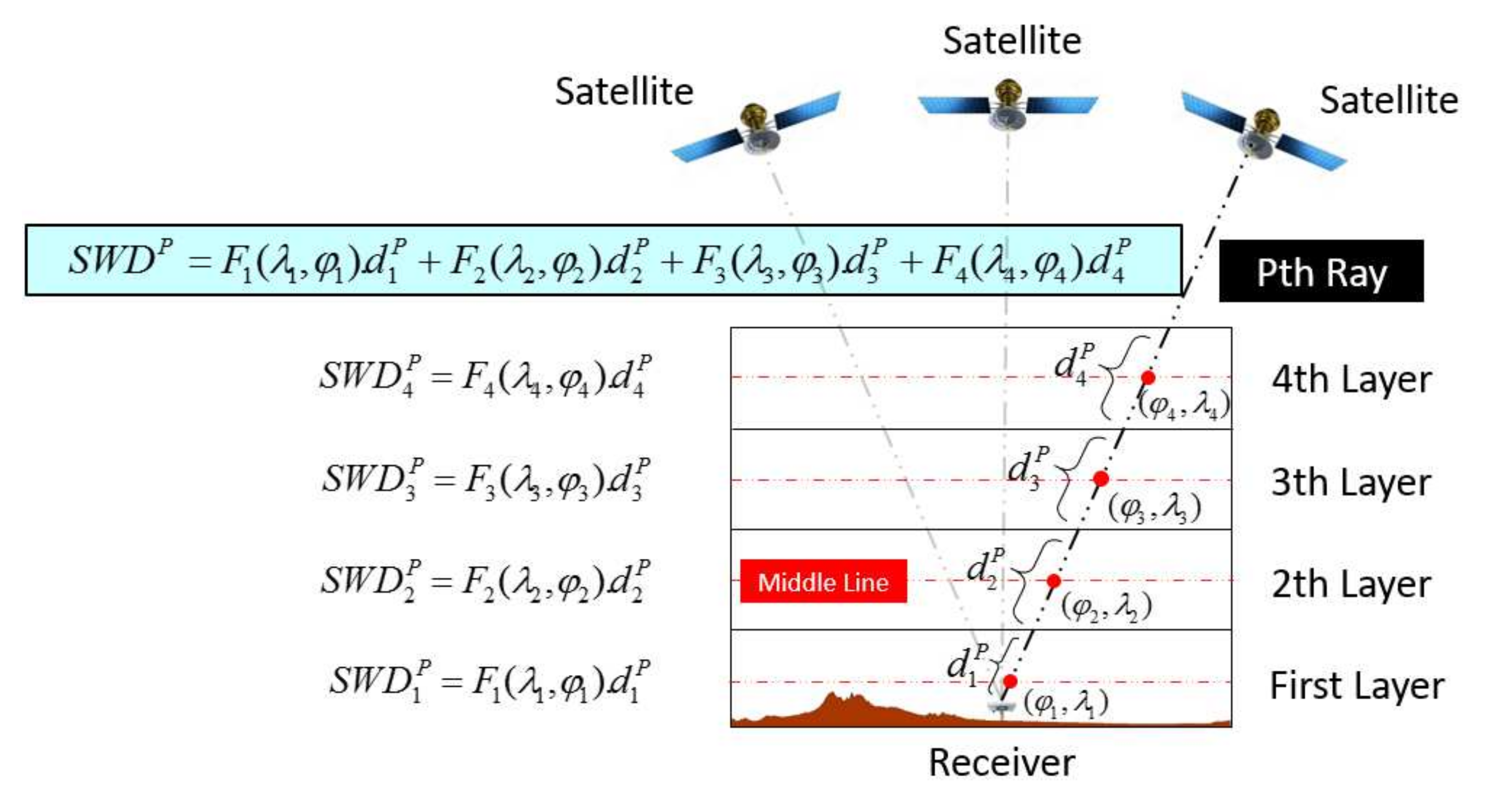
2. Function-Based Troposphere Tomography
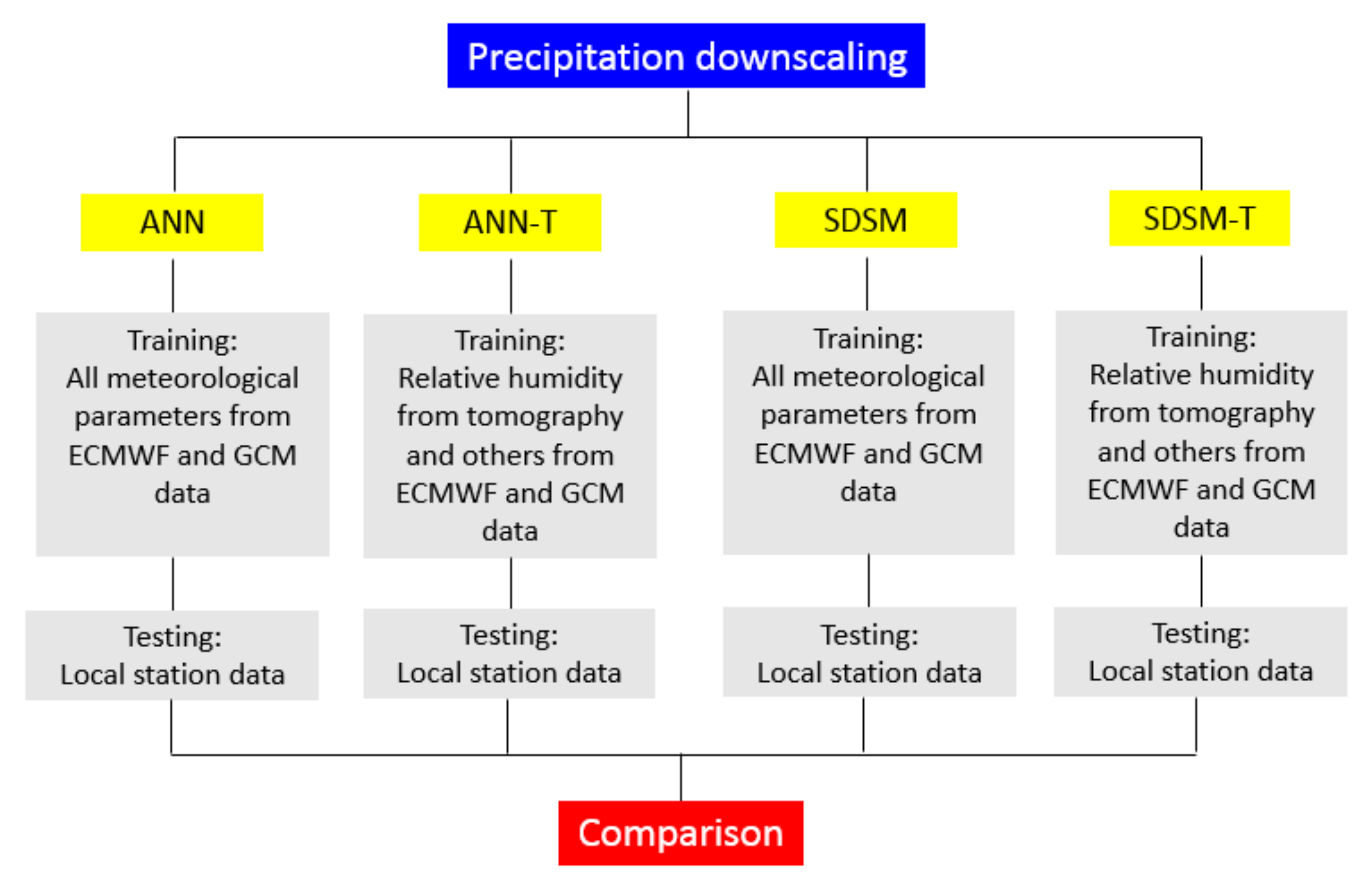
3. Downscaling Methods
3.1. SDSM
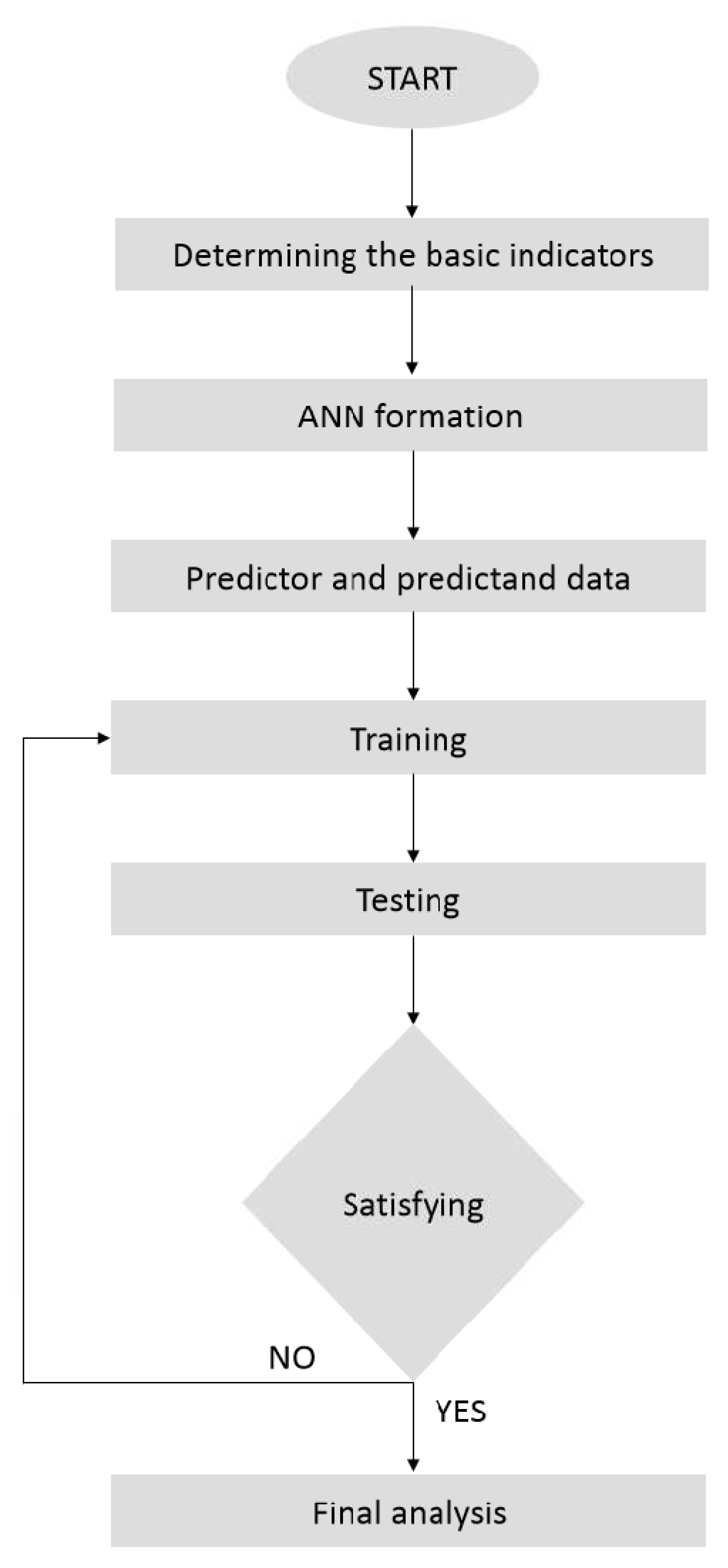
3.2. ANNs
4. Validation Methods
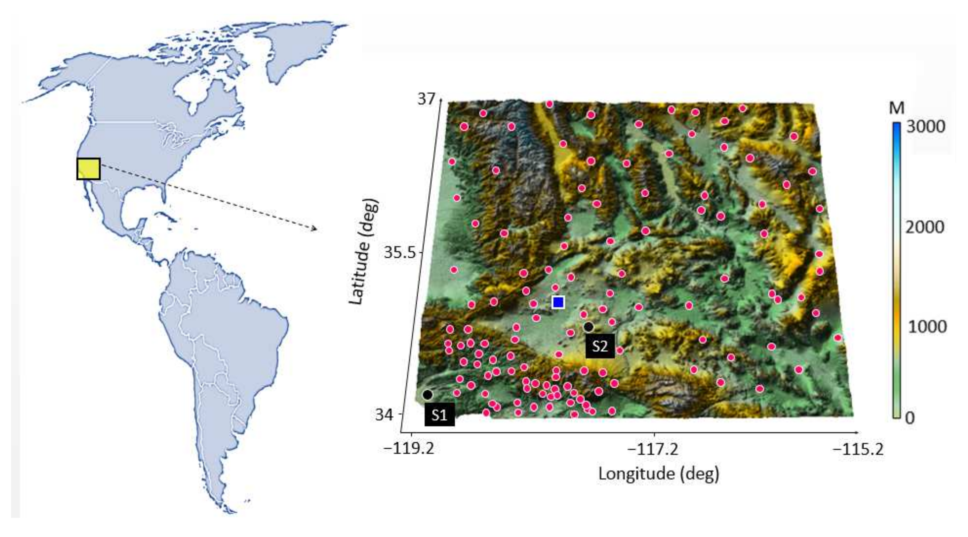
5. Study Area and Data Set
6. Processing Results and Discussions
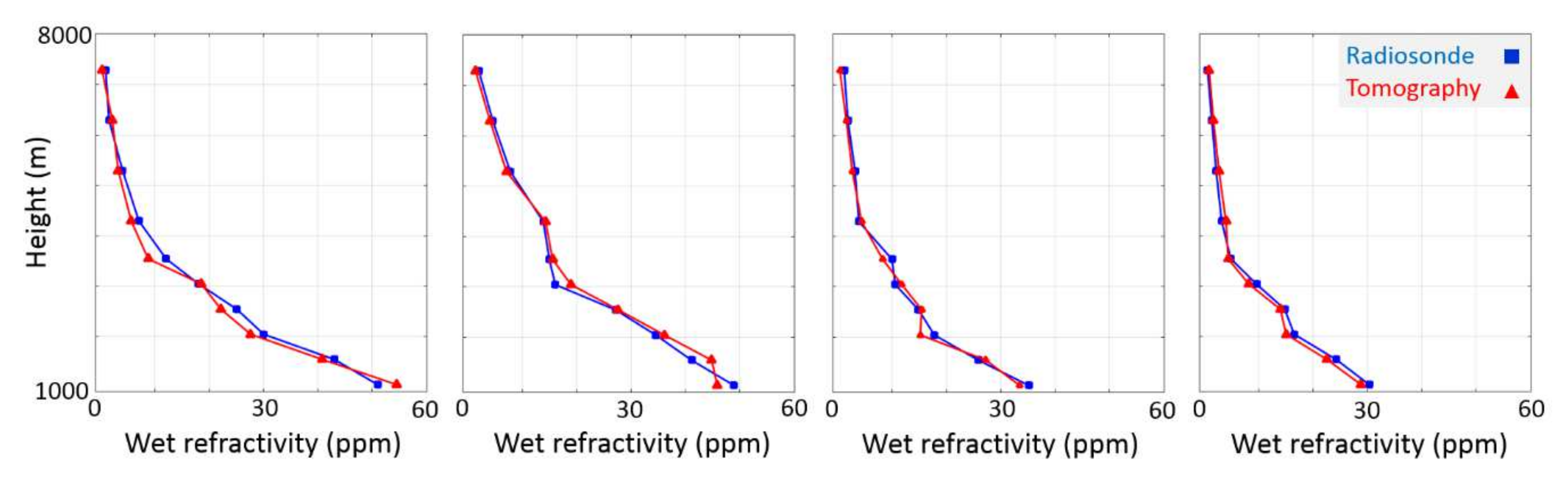
6.1. Troposphere Tomography
6.2. Downscaling of Precipitation Based on the SDSM
6.3. Downscaling of Precipitation Based on an ANN
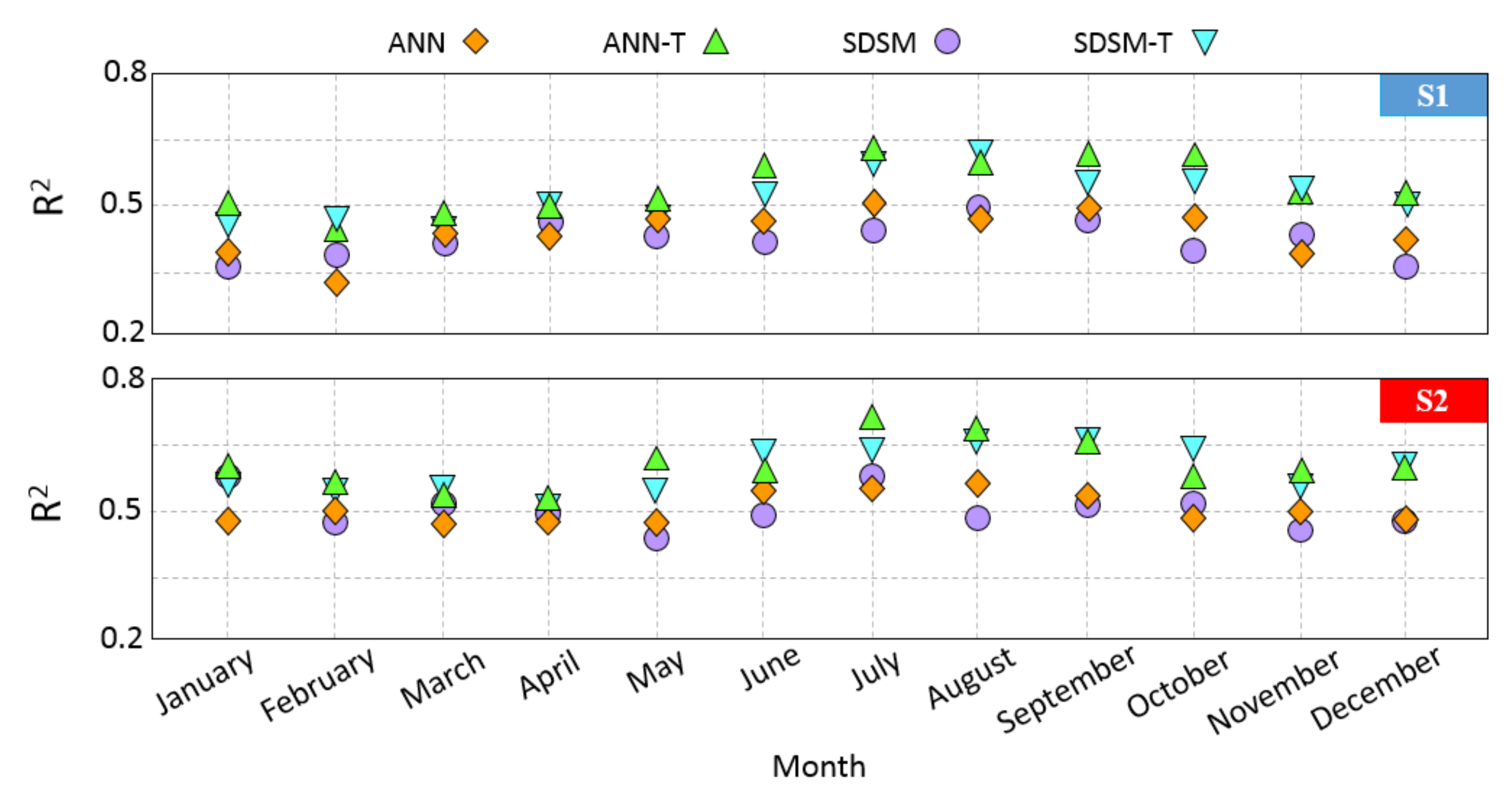
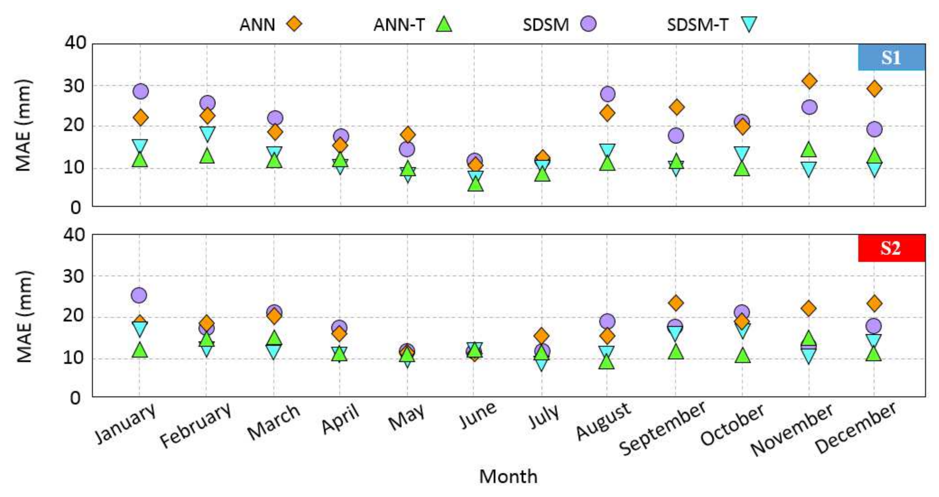
6.4. Validation and Discussions
7. Conclusions
Author Contributions
Funding
Acknowledgments
Conflicts of Interest
References
- Anagnostopoulos, G.G.; Koutsoyiannis, D.; Christofides, A.; Efstratiadis, A.; Mamassis, N. A comparison of local and aggregated climate model outputs with observed data. Hydrol. Sci. J. 2010, 55, 1094–1110. [Google Scholar] [CrossRef]
- Koutsoyiannis, D. Revisiting the global hydrological cycle: Is it intensifying? Hydrol. Earth Syst. Sci. 2020, 24, 3899–3932. [Google Scholar] [CrossRef]
- Hewitson, B.C.; Crane, R.G. Climate downscaling: Techniques and application. Clim. Res. 1996, 7, 85–95. [Google Scholar] [CrossRef]
- Xu, C.Y. From GCMs to river flow: A review of downscaling methods and hydrologic modelling approaches. Prog. Phys. Geogr. Earth Environ. 1999, 23, 229–249. [Google Scholar] [CrossRef]
- Wilby, R.L.; Charles, S.P.; Zorita, E.; Timbal, B.; Whetton, P.; Mearns, L.O. Guidelines for Use of Climate Scenarios Developed from Statistical Downscaling Methods. Supporting Material of the Intergovernmental Panel on Climate Change. The DDC of IPCC TGCIA 27. 2004. Available online: https://www.semanticscholar.org/paper/Guidelines-for-Use-of-Climate-Scenarios-Developed-Wilby-Charles/3f10e91a922860e49a42b4ee5ffa14ad7e6500e8 (accessed on 7 May 2022).
- Fowler, H.J.; Blenkinsop, S.; Tebaldi, C. Linking climate change modelling to impacts studies: Recent advances in downscaling techniques for hydrological modelling. Int. J. Climatol. 2007, 27, 1547–1578. [Google Scholar] [CrossRef]
- Semenov, M.A.; Brooks, R.J.; Barrow, E.M.; Richardson, C.W. Comparison of the WGEN and LARS-WG stochastic weather generators for diverse climates. Clim. Res. 1998, 10, 95–107. [Google Scholar] [CrossRef] [Green Version]
- Dibike, Y.B.; Coulibaly, P. Hydrologic impact of climate change in the Saguenay watershed: Comparison of downscaling methods and hydrologic models. J. Hydrol. 2005, 307, 145–163. [Google Scholar] [CrossRef]
- Kilsby, C.G.; Jones, P.D.; Burton, A.; Ford, A.C.; Fowler, H.J.; Harpham, C.; James, P.; Smith, A.; Wilby, R.L. A daily weather generator for use in climate change studies. Environ. Model. Softw. 2007, 22, 1705–1719. [Google Scholar] [CrossRef]
- Kim, B.S.; Kim, H.S.; Seoh, B.H.; Kim, N.W. Impact of climate change on water resources in Yongdam Dam Basin, Korea. Stoch. Environ. Res. Risk Assess. 2007, 21, 355–373. [Google Scholar] [CrossRef]
- Chen, S.-T.; Yu, P.-S.; Tang, Y.-H. Statistical downscaling of daily precipitation using support vector machines and multivariate analysis. J. Hydrol. 2010, 385, 13–22. [Google Scholar] [CrossRef]
- Li, X.; Li, Z.; Huang, W.; Zhou, P. Performance of statistical and machine learning ensembles for daily temperature downscaling. Arch. Meteorol. Geophys. Bioclimatol. Ser. B 2020, 140, 571–588. [Google Scholar] [CrossRef]
- Hammami, D.; Lee, T.S.; Ouarda, T.B.M.J.; Lee, J. Predictor selection for downscaling GCM data with LASSO. J. Geophys. Res. Earth Surf. 2012, 117, 211–226. [Google Scholar] [CrossRef]
- Nourani, V.; Razzaghzadeh, Z.; Baghanam, A.H.; Molajou, A. ANN-based statistical downscaling of climatic parameters using decision tree predictor screening method. Arch. Meteorol. Geophys. Bioclimatol. Ser. B 2018, 137, 1729–1746. [Google Scholar] [CrossRef]
- Singh, V.; Jain, S.K.; Singh, P.K. Inter-comparisons and applicability of CMIP5 GCMs, RCMs and statistically downscaled NEXGDDP based precipitation in India. Sci. Total Environ. 2019, 697, 134163. [Google Scholar] [CrossRef] [PubMed]
- Su, H.; Xiong, Z.; Yan, X.; Dai, X. An evaluation of two statistical downscaling models for downscaling monthly precipitation in the Heihe River basin of China. Arch. Meteorol. Geophys. Bioclimatol. Ser. B 2019, 138, 1913–1923. [Google Scholar] [CrossRef]
- Heyen, H.; Zorita, E.; Von Storch, H. Statistical downscaling of monthly mean North Atlantic air-pressure to sea level anomalies in the Baltic Sea. Tellus A Dyn. Meteorol. Oceanogr. 1996, 48, 312–323. [Google Scholar] [CrossRef] [Green Version]
- Wilby, R.L.; Dawson, C.W.; Barrow, E.M. SDSM—A decision support tool for the assessment of regional climate change impacts. Environ. Model. Softw. 2002, 17, 145–157. [Google Scholar] [CrossRef]
- Iliopoulou, T.; Koutsoyiannis, D. Projecting the future of rainfall extremes: Better classic than trendy. J. Hydrol. 2020, 588, 125005. [Google Scholar] [CrossRef]
- Lombardo, F.; Volpi, E.; Koutsoyiannis, D. Rainfall downscaling in time: Theoretical and empirical comparison between multifractal and Hurst-Kolmogorov discrete random cascades. Hydrol. Sci. J. 2012, 57, 1052–1066. [Google Scholar] [CrossRef] [Green Version]
- Dimitriadis, P.; Koutsoyiannis, D.; Iliopoulou, T.; Papanicolaou, P. A Global-Scale Investigation of Stochastic Similarities in Marginal Distribution and Dependence Structure of Key Hydrological-Cycle Processes. Hydrology 2021, 8, 59. [Google Scholar] [CrossRef]
- Kourgialas, N.N.; Dokou, Z.; Karatzas, G.P. Statistical analysis and ANN modeling for predicting hydrological extremes under climate change scenarios: The example of a small Mediterranean agro-watershed. J. Environ. Manag. 2015, 154, 86–101. [Google Scholar] [CrossRef] [PubMed]
- Rozos, E.; Dimitriadis, P.; Mazi, K.; Koussis, A. A Multilayer Perceptron Model for Stochastic Synthesis. Hydrology 2021, 8, 67. [Google Scholar] [CrossRef]
- Rozos, E.; Dimitriadis, P.; Bellos, V. Machine Learning in Assessing the Performance of Hydrological Models. Hydrology 2021, 9, 5. [Google Scholar] [CrossRef]
- Shenify, M.; Danesh, A.S.; Gocić, M.; Taher, R.S.; Wahab, A.W.A.; Gani, A.; Shamshirband, S.; Petković, D. Precipitation Estimation Using Support Vector Machine with Discrete Wavelet Transform. Water Resour. Manag. 2015, 30, 641–652. [Google Scholar] [CrossRef]
- Wang, Q.; Huang, J.; Liu, R.; Men, C.; Guo, L.; Miao, Y.; Jiao, L.; Wang, Y.; Shoaib, M.; Xia, X. Sequence-based statistical downscaling and its application to hydrologic simulations based on machine learning and big data. J. Hydrol. 2020, 586, 124875. [Google Scholar] [CrossRef]
- Flores, A.; Ru_ni, G.; Rius, A. 4D tropospheric tomography using GPS slant wet delays. Ann. Geophys. 2000, 18, 223–234. [Google Scholar] [CrossRef]
- Rohm, W.; Bosy, J. Local tomography troposphere model over mountains area. Atmos. Res. 2009, 93, 777–783. [Google Scholar] [CrossRef]
- Aghajany, S.H.; Amerian, Y. Three dimensional ray tracing technique for tropospheric water vapor tomography using GPS measurements. J. Atmos. Sol. Terr. Phys. 2017, 164, 81–88. [Google Scholar] [CrossRef]
- Haji-Aghajany, S.; Amerian, Y. Hybrid Regularized GPS Tropospheric Sensing Using 3-D Ray Tracing Technique. IEEE Geosci. Remote Sens. Lett. 2018, 15, 1475–1479. [Google Scholar] [CrossRef]
- Haji-Aghajany, S.; Amerian, Y.; Verhagen, S.; Rohm, W.; Ma, H. An Optimal Troposphere Tomography Technique Using the WRF Model Outputs and Topography of the Area. Remote Sens. 2020, 12, 1442. [Google Scholar] [CrossRef]
- Brenot, H.; Rohm, W.; Kačmařík, M.; Möller, G.; Sá, A.; Tonda´s, D.; Rapant, L.; Biondi, R.; Manning, T.; Champollion, C. Cross-Comparison and Methodological Improvement in GPS Tomography. Remote Sens. 2019, 12, 30. [Google Scholar] [CrossRef] [Green Version]
- Haji-Aghajany, S.; Amerian, Y.; Verhagen, S. B-spline function-based approach for GPS tropospheric tomography. GPS Solut. 2020, 24, 88. [Google Scholar] [CrossRef]
- Haji-Aghajany, S.; Amerian, Y.; Verhagen, S.; Rohm, W.; Schuh, H. The effect of function-based and voxel-based tropospheric tomography techniques on the GNSS positioning accuracy. J. Geod. 2021, 95, 78. [Google Scholar] [CrossRef]
- Braun, J.J. Remote Sensing of Atmospheric Water Vapor with the Global Positioning System. Ph.D. Thesis, University of Colorado, Boulder, CO, USA, 2004. [Google Scholar]
- Bevis, M.; Businger, S.; Herring, T.A.; Rocken, C.; Anthes, R.A.; Ware, R.H. GPS meteorology: Remote sensing of atmospheric water vapor using the global positioning system. J. Geophys. Res. Atmos. 1992, 97, 15787–15801. [Google Scholar] [CrossRef]
- Davis, J.; Elgered, G.; Niell, A.E.; Kuehn, C.E. Ground-based measurement of gradients in the “wet” radio refractivity of air. Radio Sci. 1993, 28, 1003–1018. [Google Scholar] [CrossRef]
- Chen, B.Y.; Liu, Z.Z. Voxel-optimized regional water vapor tomography and comparison with radiosonde and numerical weather model. J. Geod. 2014, 88, 691–703. [Google Scholar] [CrossRef]
- Troller, M.; Bürki, B.; Cocard, M.; Geiger, A.; Kahle, H.-G. 3-D refractivity field from GPS double difference tomography. Geophys. Res. Lett. 2002, 29, 2-1–2-4. [Google Scholar] [CrossRef]
- Bender, M.; Dick, G.; Ge, M.; Deng, Z.; Wickert, J.; Kahle, H.-G.; Raabe, A.; Tetzlaff, G. Development of a GNSS water vapour tomography system using algebraic reconstruction techniques. Adv. Space Res. 2011, 47, 1704–1720. [Google Scholar] [CrossRef] [Green Version]
- Amerian, Y.; Hossainali, M.M.; Voosoghi, B. Regional improvement of IRI extracted ionospheric electron density by compactly supported base functions using GPS observations. J. Atmos. Sol. Terr. Phys. 2013, 92, 23–30. [Google Scholar] [CrossRef]
- De Boor, C. On calculating with B-splines. J. Approx. Theory 1972, 6, 50–62. [Google Scholar] [CrossRef] [Green Version]
- Elósegui, P.; Ruis, A.; Davis, J.; Ruffini, G.; Keihm, S.; Bürki, B.; Kruse, L. An experiment for estimation of the spatial and temporal variations of water vapor using GPS data. Phys. Chem. Earth 1998, 23, 125–130. [Google Scholar] [CrossRef]
- Magee, L. Nonlocal Behavior in Polynomial Regressions. Am. Stat. 1998, 52, 20. [Google Scholar] [CrossRef]
- Amerian, Y.; Voosoghi, B.; Hossainali, M.M. Regional ionosphere modeling in support of IRI and wavelet using GPS observations. Acta Geophys. 2013, 61, 1246–1261. [Google Scholar] [CrossRef]
- Hardy, B. ITS-90 Formulations for Water Vapor Pressure, Frostpoint Temperature, Dewpoint Temperature, and Enhancement Factors in range −100 to +100 C. In Proceedings of the Third International Symposium on Humidity and Moisture, Teddington, UK, 6–8 April 1998; pp. 1–8. [Google Scholar]
- Mateus, P.; Mendes, V.; Plecha, S. HGPT2: An ERA5-Based Global Model to Estimate Relative Humidity. Remote Sens. 2021, 13, 2179. [Google Scholar] [CrossRef]
- Hansen, P.C. Rank-Deficient and Discrete Ill-Posed Problems. Numerical Aspects of Linear Inversion, Monographs on Mathematical Modeling and Computation; SIAM: Philadelphia, PA, USA, 1997; Volume 4. [Google Scholar]
- Haji-Aghajany, S.; Voosoghi, B.; Amerian, Y. Estimating the slip rate on the north Tabriz fault (Iran) from InSAR measurements with tropospheric correction using 3D ray tracing technique. Adv. Space Res. 2019, 64, 2199–2208. [Google Scholar] [CrossRef]
- Haji-Aghajany, S.; Amerian, Y. An investigation of three dimensional ray tracing method efficiency in precise point positioning by tropospheric delay correction. J. Earth Space Phys. 2018, 44, 39–52. [Google Scholar] [CrossRef]
- Abdelwares, M.; Haggag, M.; Wagdy, A.; Lelieveld, J. Customized framework of the WRF model for regional climate simulation over the Eastern NILE basin. Arch. Meteorol. Geophys. Bioclimatol. Ser. B 2017, 134, 1135–1151. [Google Scholar] [CrossRef]
- Rahman Hashmi, M.Z.U.; Shamseldin, A.Y.; Melville, B.W. Comparison of MLP-ANN Scheme and SDSM as Tools for Providing Downscaled Precipitation for Impact Studies at Daily Time Scale. J. Earth Sci. Clim. Chang. 2018, 9, 1–4. [Google Scholar] [CrossRef]
- Wilby, R.; Hay, L.; Leavesley, G. A comparison of downscaled and raw GCM output: Implications for climate change scenarios in the San Juan River basin, Colorado. J. Hydrol. 1999, 225, 67–91. [Google Scholar] [CrossRef]
- Wilby, R.L.; Tomlinson, O.J.; Dawson, C. Multi-site simulation of precipitation by conditional resampling. Clim. Res. 2003, 23, 183–194. [Google Scholar] [CrossRef]
- Haykin, S. Neural Networks: A Comprehensive Foundation, 2nd ed.; Prentice-Hall: Englewood Cliffs, NJ, USA; New York, NY, USA, 1999. [Google Scholar]
- Ahmed, K.; Shahid, S.; Bin Haroon, S.; Xiao-Jun, W. Multilayer perceptron neural network for downscaling rainfall in arid region: A case study of Baluchistan, Pakistan. J. Earth Syst. Sci. 2015, 124, 1325–1341. [Google Scholar] [CrossRef] [Green Version]
- Hornik, K.; Stinchcombe, M.; White, M. Multilayer feed forward networks are universal approximates. Neural Netw. 1989, 2, 359–366. [Google Scholar] [CrossRef]
- Levenberg, K. A method for the solution of certain non-linear problems in least squares. Q. Appl. Math. 1944, 2, 164–168. [Google Scholar] [CrossRef] [Green Version]
- Marquardt, D.W. An Algorithm for Least-Squares Estimation of Nonlinear Parameters. J. Soc. Ind. Appl. Math. 1963, 11, 431–441. [Google Scholar] [CrossRef]
- Banerjee, P.; Prasad, R.K.; Singh, V.S. Forecasting of groundwater level in hard rock region using artificial neural network. Environ. Earth Sci. 2008, 58, 1239–1246. [Google Scholar] [CrossRef]
- Chang, J.; Wang, G.; Mao, T. Simulation and prediction of supra permafrost groundwater level variation in response to climate change using a neural network model. J. Hydrol. 2015, 529, 1211–1220. [Google Scholar] [CrossRef]
- Moriasi, D.N.; Arnold, J.G.; van Liew, M.W.; Bingner, R.L.; Harmel, R.D.; Veith, T.L. Model evaluation guidelines for systematic quantification of accuracy in watershed simulations. Trans. ASABE 2007, 50, 885–900. [Google Scholar] [CrossRef]
- Hersbach, H.; Dee, D. ERA5 Reanalysis is in Production; ECMWF Newsletter 147; ECMWF: Reading, UK, 2016. [Google Scholar]
- Haji-Aghajany, S.; Amerian, Y. Atmospheric phase screen estimation for land subsidence evaluation by InSAR time series analysis in Kurdistan, Iran. J. Atmos. Sol. Terr. Phys. 2020, 205, 105314. [Google Scholar] [CrossRef]
- Haji-Aghajany, S.; Amerian, Y. Assessment of InSAR tropospheric signal correction methods. J. Appl. Remote Sens. 2020, 14, 044503. [Google Scholar] [CrossRef]
- Aghajany, S.H.; Voosoghi, B.; Yazdian, A. Estimation of north Tabriz fault parameters using neural networks and 3D tropospherically corrected surface displacement field. Geomat. Nat. Hazards Risk 2017, 8, 918–932. [Google Scholar] [CrossRef] [Green Version]
- Dach, R.; Lutz, S.; Walser, P.; Fridez, P. (Eds.) Bernese GNSS Software Version 5.2. User Manual; Astronomical Institute, University of Bern; Bern Open Publishing: Bern, Switzerland, 2015; ISBN 978-3-906813-05-9. [Google Scholar] [CrossRef]
- Böhm, J.; Niell, A.; Tregoning, P.; Schuh, H. Global Mapping Function (GMF): A new empirical mapping function based on numerical weather model data. Geophys. Res. Lett. 2006, 33, 1–4. [Google Scholar] [CrossRef] [Green Version]


| RMSE (ppm) | Bias (ppm) | Min-Diff (ppm) | Max-Diff (ppm) |
|---|---|---|---|
| 2.26 | 0.46 | 0.09 | 5.78 |
| Training Algorithm | S1 | S2 | ||||
|---|---|---|---|---|---|---|
| RMSE | NSE | R2 | RMSE | NSE | R2 | |
| GD | 7.412 | 0.178 | 0.746 | 7.98 | 0.311 | 0.846 |
| LM | 0.368 | 0.954 | 0.972 | 0.399 | 0.961 | 0.942 |
| BFGS | 0.521 | 0.924 | 0.911 | 0.475 | 0.901 | 0.881 |
| CGF | 0.784 | 0.913 | 0.831 | 0.739 | 0.919 | 0.883 |
| Model Number | Number of Hidden Layers | Number of Neurons in the First Layer | Number of Neurons in the Second Layer | RMSE | NSE | R2 |
|---|---|---|---|---|---|---|
| 1 | 1 | 2 | - | 0.597 | 0.953 | 0.891 |
| 2 | 1 | 6 | - | 0.574 | 0.942 | 0.893 |
| 3 | 1 | 12 | - | 0.458 | 0.962 | 0.898 |
| 4 | 1 | 18 | - | 0.524 | 0.949 | 0.889 |
| 5 | 2 | 2 | 2 | 0.584 | 0.954 | 0.898 |
| 6 | 2 | 4 | 6 | 0.612 | 0.963 | 0.901 |
| 7 | 2 | 6 | 8 | 0.574 | 0.951 | 0.902 |
| 8 | 2 | 8 | 8 | 0.404 | 0.964 | 0.901 |
| 9 | 2 | 10 | 10 | 0.531 | 0.943 | 0.914 |
| 10 | 2 | 14 | 8 | 0.438 | 0.963 | 0.891 |
| ANN Type | Number of Neurons | Stimulus Function of Hidden Layers | Stimulus Function of Output Layers | Training Algorithm |
|---|---|---|---|---|
| Three-layer feed-forward MLP | 8-8 | tangent and sigmoid log | Linear | LM |
| Indicator | Month | S1 | S2 | ||||||
|---|---|---|---|---|---|---|---|---|---|
| ANN | ANN-T | SDSM | SDSM-T | ANN | ANN-T | SDSM | SDSM-T | ||
| RMSE (mm) | January | 29.24 | 11.47 | 30.12 | 15.87 | 17.69 | 10.84 | 25.51 | 18.08 |
| February | 20.15 | 14.34 | 23.57 | 17.66 | 28.29 | 12.43 | 29.52 | 15.68 | |
| March | 27.36 | 13.74 | 24.89 | 13.42 | 20.91 | 13.28 | 23.64 | 14.27 | |
| April | 17.58 | 10.43 | 23.74 | 14.08 | 15.94 | 10.07 | 14.51 | 11.87 | |
| May | 19.46 | 14.84 | 17.49 | 16.19 | 16.83 | 11.92 | 15.03 | 11.27 | |
| June | 12.81 | 10.45 | 10.74 | 09.86 | 11.83 | 10.93 | 12.39 | 12.84 | |
| July | 13.87 | 11.43 | 15.76 | 14.79 | 13.24 | 12.51 | 14.84 | 13.63 | |
| August | 31.47 | 18.23 | 32.11 | 21.63 | 21.52 | 11.36 | 23.87 | 13.96 | |
| September | 33.88 | 14.21 | 24.31 | 16.75 | 26.82 | 13.87 | 22.26 | 12.73 | |
| October | 26.89 | 17.28 | 30.05 | 21.49 | 23.83 | 15.86 | 25.74 | 12.18 | |
| November | 38.23 | 16.71 | 35.61 | 20.72 | 27.84 | 18.42 | 20.68 | 18.91 | |
| December | 32.39 | 16.34 | 25.46 | 18.53 | 28.93 | 19.88 | 26.79 | 16.64 | |
| Average (mm) | All months | 25.27 | 14.12 | 24.48 | 16.74 | 21.13 | 13.14 | 21.23 | 14.33 |
Publisher’s Note: MDPI stays neutral with regard to jurisdictional claims in published maps and institutional affiliations. |
© 2022 by the authors. Licensee MDPI, Basel, Switzerland. This article is an open access article distributed under the terms and conditions of the Creative Commons Attribution (CC BY) license (https://creativecommons.org/licenses/by/4.0/).
Share and Cite
Haji-Aghajany, S.; Amerian, Y.; Amiri-Simkooei, A. Function-Based Troposphere Tomography Technique for Optimal Downscaling of Precipitation. Remote Sens. 2022, 14, 2548. https://doi.org/10.3390/rs14112548
Haji-Aghajany S, Amerian Y, Amiri-Simkooei A. Function-Based Troposphere Tomography Technique for Optimal Downscaling of Precipitation. Remote Sensing. 2022; 14(11):2548. https://doi.org/10.3390/rs14112548
Chicago/Turabian StyleHaji-Aghajany, Saeid, Yazdan Amerian, and Alireza Amiri-Simkooei. 2022. "Function-Based Troposphere Tomography Technique for Optimal Downscaling of Precipitation" Remote Sensing 14, no. 11: 2548. https://doi.org/10.3390/rs14112548