Abstract
Maize is one of the most important crops in China, and it is under a serious, ever-increasing threat from southern corn rust (SCR). The identification of wheat rust based on hyperspectral data has been proved effective, but little research on detecting maize rust has been reported. In this study, full-range hyperspectral data (350~2500 nm) were collected under solar illumination, and spectra collected under solar illumination (SCUSI) were separated into several groups according to the disease severity, measuring height and leaf curvature (the smoothness of the leaf surface). Ten indices were selected as candidate indicators for SCR classification, and their sensitivities to the disease severity, measuring height and leaf curvature, were subjected to analysis of variance (ANOVA). The better-performing indices according to the ANOVA test were applied to a random forest classifier, and the classification results were evaluated by using a confusion matrix. The results indicate that the PRI was the optimal index for SCR classification based on the SCUSI, with an overall accuracy of 81.30% for mixed samples. The results lay the foundation for SCR detection in the incubation period and reveal potential for SCR detection based on UAV and satellite imageries, which may provide a rapid, timely and cost-effective detection method for SCR monitoring.
1. Introduction
Corn (also called maize) is one of the major crops in the world, and its yield was 1148 million tons in 2019 [1]. In China, maize production has far surpassed that of other major crops [2]. However, the loss of maize yield induced by diseases has increased due to a lack of host resistance. Among all the maize diseases, southern corn rust (SCR) attracts increasing attention because of its wider spread and heavier damage. SCR is caused by Puccinia polysora Underw., an obligate biotrophic parasite. Each year, the pathogen’s spores spread from tropical areas to extratropical regions and cause epidemics in the major maize-producing areas. Therefore, a rapid, precise method of detection for SCR is crucial for plant protection and disease control.
The methods commonly used for disease diagnosis consist of (1) artificial visual investigation based on disease symptoms in the field [3]; (2) the observation of the pathogen under a microscope in the laboratory [4]; and (3) disease detection based on molecular techniques [5]. The first method is the traditional investigation method and has been used for decades by virtue of its simplicity. However, field investigation relies on professional knowledge, and the similarity of symptoms may cause misjudgment. In addition, early detection cannot be achieved by traditional investigation, as the symptoms typically manifest in the middle-to-later stages of the infection. The characteristics of the pathogen under a microscope are a more reliable indicator for disease identification, and earlier diagnosis can be performed. Nevertheless, it still relies on a priori knowledge, and the process is time-consuming. Molecular-based methods can provide precise detection results, and the pathogens can be diagnosed during the incubation period [6]. However, this method is costly, and the process from sampling to obtaining the result takes several days, leading to low efficiency. In order to better implement plant protection policies and reduce the yield losses caused by diseases, a cost-effective, real-time detection method is required.
The invasion of the pathogen and its development in mesophyll cells [7] can cause changes in the leaf’s inner structure and a decrease in the chlorophyll, anthocyanin and water contents [8,9]. These physical and chemical changes can be embodied in the reflectances of infected leaves. Hyperspectral data contain reflectance information spanning a wide spectral range (350~2500 nm, far beyond that of human vision) and, hence, have the potential to enable the detection of subtle changes in plant growth [10]. The wide spectral range can be divided into four parts: visible (VIS, 390~690 nm [11,12]), red edge (690~750 nm [12]), near infrared (NIR, 750~1300 nm [13]) and shortwave infrared (SWIR, 1300~2500 nm [13]). For visible bands, especially the red band (620~690 nm), as pathogens can destroy the chlorophyll after infection, the absorption of red light by the chloroplast declines, resulting in higher reflectance values in the red range. The red edge is another spectral range that has been used to identify diseases. In the red-edge range, a sharp change in reflectance is the obvious characteristic. Infection with the disease can change the position and shape of this range [14], and the change commonly occurs earlier than that of the visible band [15]. The multiple scattering of radiation in the leaf mesophyll causes high reflectance in the NIR. The intracellular and intercellular structural changes caused by pathogens can reduce the reflectance in the NIR range. The reflectance in the SWIR range is closely related to the water content. The water content decreases with the development of the pathogen, which can be used as an indicator for disease identification.
A typical disease-monitoring process includes the following steps: (1) feature (i.e., the dimension of input data) construction; (2) feature selection and model determination; and (3) accuracy evaluation. In step one, the features can be the raw reflectance or other transformed parameters. To reduce the data dimensions, researchers have preferred to select sensitive bands by using spectral curve analysis or specific models [16] rather than applying all the original reflectance [17]. Transformed features acquired by index calculations [18], derivatives [19] and wavelet transformation [20] have also been widely adopted; index construction is the simplest method and is effective. As a result, numerous indices have been reported to date [21]; specifically, Meng et al. [22] established two SCR-specific indices for SCR detection and classification. In step two, some analysis methods, such as analysis of variance (ANOVA) [23], can only select a target feature by evaluating the sensitivity to disease severity, while other methods, such as classification (for categorical variables) and regression (for continuous variables) algorithms, can achieve feature selection and model construction simultaneously. The commonly used classification methods include random forest (RF) [24], support vector machine (SVM) [22], K-nearest neighbor (KNN) [25], etc. Regarding regression models, the most classical one is partial least-square regression (PLSR) [20]. Support vector regression (SVR) [26] has been used as an alternative regression method when the linear regression method does not work well, as the SVR can describe the inherent nonlinear relationship between input and output datasets [27]. In step three, the accuracy evaluation method varies according to the type of variable. A confusion matrix has been applied when dealing with categorical variables, and the descriptions of the confusion matrix are not identical in different research fields. The parameters of the confusion matrix were described as the overall accuracy (OA), kappa coefficient, user accuracy and mapping accuracy in studies on RS imagery classification [28]. The parameters were called the overall accuracy (OA), recall, precision, F1 score, macro average of precision (MAP), macro average of recall (MAR), weighted average of precision (WAP) and weighted average of recall (WAR) in machine learning model evaluations [29]. For continuous variables, the coefficient of correlation (r) and root mean square error (RMSE) were the two main evaluation parameters [30].
With the development of soft computing, more and more advanced methods, such as genetic programming (GM), functional data analysis (FDA), the technique for order of preference by similarity to ideal solution (TOPSIS), group method of data handling (GMDH), artificial neural network (ANN) and adaptive neuro fuzzy inference system, (ANFIS) have been applied in studies. The most obvious characteristics of advanced methods are their lower subjectivity and the fact that the feature construction and feature selection process can be carried out automatically. For example, Albarracín et al. [31] proposed a genetic-programming-based vegetation index (GPVI) based on an evolution rule and fitness algorithm. Compared with the traditional normalized difference vegetation index (NDVI) and enhanced vegetation index (EVI), the GPVI had no fixed formula and automatically varied with the classification task. Functional data analysis (FDA) is another useful feature extraction method. Unlike traditional statistical analysis, FDA treats multivariate data (e.g., hyperspectral curves) as continuous functions, which can make full use of the abundant spectral information. Li et al. [32] analyzed hyperspectral data by using FDA, and a series of functional features were created. Based on these functional features, an SVM classifier achieved a higher accuracy in a hyperspectral imagery classification task. Apart from applications in stress detection, soft computing technology has been applied in wider areas, especially in the monitoring of natural phenomena such as wave heights [33,34], water quality [35], gully erosion susceptibility [36] and landslide susceptibility [37]. Other technologies have also been applied in studies. For example, Esposito et al. [38] recently completed studies about sustainable weed management based on drone and sensor technology. Dal-Sasso et al. [39] monitored the dynamics of surface flow velocity by using an image-processing method called particle-tracking velocimetry (PTV).
Based on various methods, many studies and researchers have adopted RS-based methods for disease detection in a range of crops, such as rice [40], wheat [41], maize [22], potatoes [42,43], peanuts [44] and soybeans [45]. Rust was one of the earliest diseases monitored by remote sensing, especially wheat rust. Moshou et al. [46] attempted to detect wheat yellow rust (i.e., wheat stripe rust) based on a neural network algorithm, and the desirable results prove the efficiency of hyperspectral data for disease detection. After that, more related articles were reported, and the studies expanded to the early detection of wheat stripe rust [47], disease severity classification [48], detection based on canopy data [49] and discrimination between yellow rust and brown rust (i.e., stem rust) [50]. Articles about wheat yellow rust monitoring based on UAV [51] and satellite imageries [52] have also been reported.
In most of the previous research, corn rust detection based on hyperspectral data has rarely been reported [22]; researchers have focused more on other maize diseases [17,53,54]. In terms of leaf-level disease classification, few papers have discussed the use of spectra collected under solar illumination (SCUSI) with a full spectral range (350~2500 nm) for disease detection because of the instability in the SWIR range caused by water vapor. In addition, in the middle-to-late growing stage, the maize leaf becomes partially curly and wrinkled. For SCUSI, the reflectance values of wrinkled areas and flat areas are significantly different, and the effect of the leaf curvature (the smoothness of the leaf surface) has not been analyzed yet. In this study, we selected ten typical stress-related indices and evaluated their sensitivities to the disease severity, measuring height and leaf curvature. The optimal index for SCR classification based on SCUSI was finally determined. The highlights of this study were (1) proposing a two-step preprocessing procedure for SCUSI with a full spectral range; (2) determining a reliable measuring height for SCUSI; (3) demonstrating that the significant variation in reflectance induced by leaf curvature can be eliminated by using proper indices and, therefore, that hyperspectral data can be collected without fixing the blades strictly flat; (4) revealing the low reliability of SCUSI in the SWIR range; and (5) determining a reliable index that performed well for SCUSI.
2. Materials and Methods
2.1. Experimental Site and Plot Design
Experiments were performed at the China Agriculture University Experimental Station, in the southeast of Xinghuaying Town, Longting District, Kaifeng City, Henan Province. Maize is sowed in early June and harvested in late September annually. The land in the study site is flat, and the soil is fertile. Due to its good infrastructure, irrigation and other agricultural operations can be carried out conveniently. Southern corn rust spores cannot overwinter in Henan Province, and their natural occurrence relies on the transmission of urediniospores from the tropical region, which leads to uncertainty in when the disease will occur and its severity. Therefore, artificial inoculation was performed before hyperspectral data acquisition.
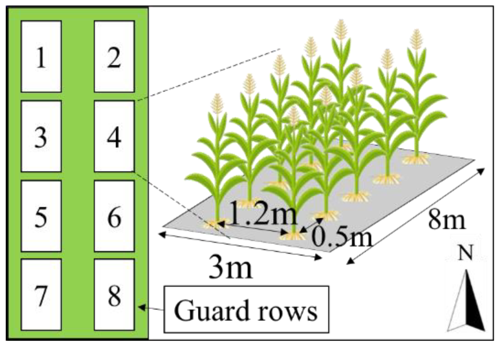
In this study, 8 field plots were designed (Figure 1). Each plot was 8 m long and 3 m wide; the line spacing and row spacing were 1.2 and 0.5 m, respectively. Each plot was separated by at least 3 guard rows. The maize variety was ZD958, a cultivar widely cultivated in North China, which is susceptible to Puccinia polysora (the pathogen that causes SCR). Plots 1–6 were inoculated by spraying a spore solution on 9 August 2021; the inoculation spores were collected from Guangxi Province, where southern corn rust had occurred one month previously. Pure water was sprayed in Plots 7–8 for comparison. Other agricultural operations, such as the application of water, fertilizers and pesticides (not fungicides), were the same throughout the growing season.

Figure 1.
Diagram of experimental plots.
2.2. Overall Workflow
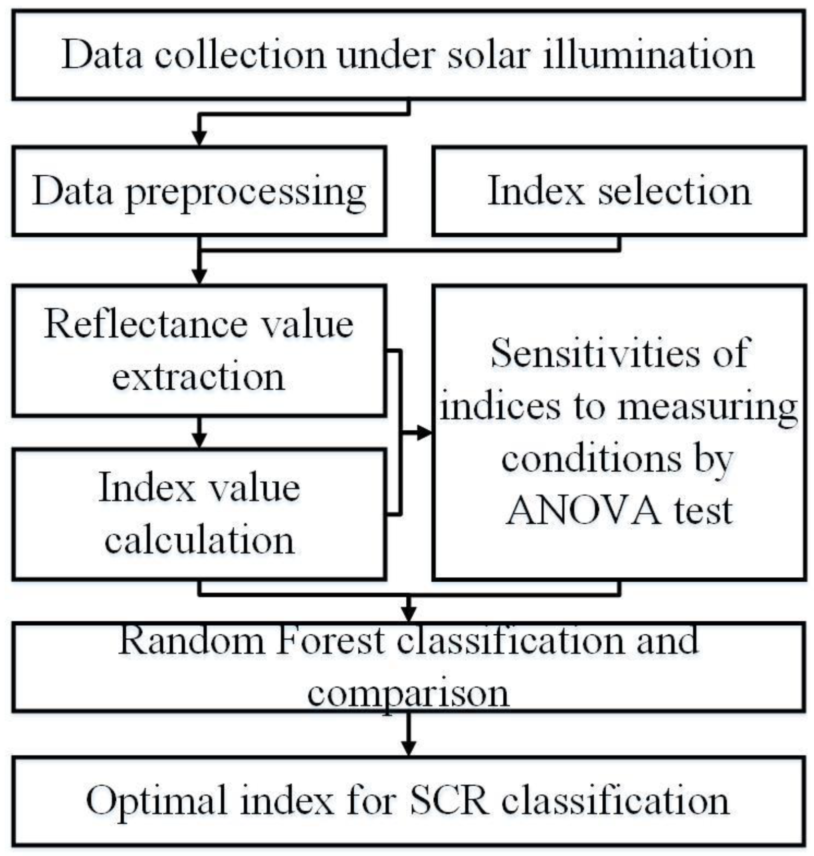
The beginning of the workflow (Figure 2) was hyperspectral data collection, after which data processing and the index selection procedure were conducted separately. The reflectance values were extracted, and the index values were calculated afterwards. One-way analysis of variance (ANOVA) tests were applied to both the reflectance values and index values. Based on the ANOVA results, indices with poor performance were omitted, and other indices were used as the input data in the random forest classification procedure. A confusion matrix was adopted to evaluate the classification results, and the optimal index was finally determined.
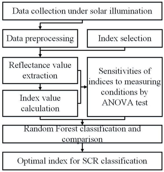
Figure 2.
Overall workflow of this study.
2.3. Data Collection
A portable field ASD Field Spec FR spectrometer was used to acquire hyperspectral data. The spectrometer covers a wide range (350~2500 nm). The spectral resolutions of the spectrometer are 3 nm for the region 350~1000 nm and 10 nm for the region 1000~2500 nm [55]. The resolutions for all the bands were resampled to 1 nm by using ViewSpecPro, a piece of software provided by the ASD corporation. For each leaf, 3 replicate measurements were conducted, and the average was taken as the final reflectance. To avoid errors induced by the leaf structure, only leaves with disease symptoms in the middle area were selected for data measurement. To minimize the effect of dark drift from the spectrometer, preopen for 15 min was carried out before data collection. In addition, white panel calibration was conducted every 5 min. Collection was performed from 11:00 to 13:00 (local time) on cloud-free days, and the other operations strictly followed the user guide provided by the ASD corporation [55].
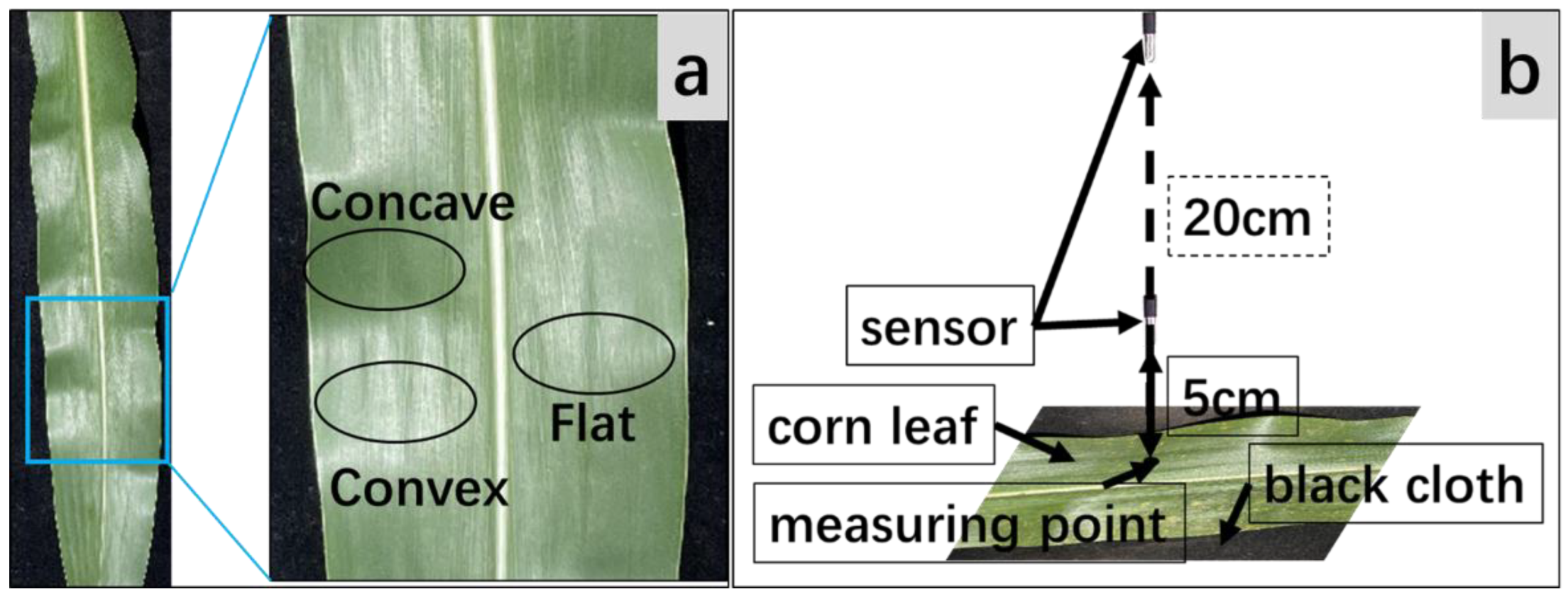
The measurements recorded under natural illumination were more sophisticated than the measurements taken with a fore optic [22] or leaf clip [48]. To suppress the effects of the incident angle and surrounding objects, the corn leaf was placed horizontally on a piece of black cloth attached to a plastic board. As the maize leaves were partially wrinkled and curly, the effects of the leaf curvature (i.e., the smoothness of the leaf surface) could not be ignored. In this study, the leaf curvature was classified into 3 types: flat (the target area was locally flat when the blade was placed horizontally), convex (the target area was locally convex when the blade was placed horizontally) and concave (the target area was locally concave when the blade was placed horizontally) (Figure 3a). In terms of the measuring height, as the field of view (FOV) of the bare fiber-optic cable was 25 degrees, the measuring area was a circle with a diameter that was 0.44 times the measuring height. Considering that the width of the maize leaf was about 10~15 cm, the diameter of the measuring area should be less than 4 cm in order to avoid the effect of the leaf vein. According to calculations, 5 cm above the corn leaf was selected as the fundamental height. Measurements at a height of 20 cm [17] above the leaf surface were taken for comparison (Figure 3b).
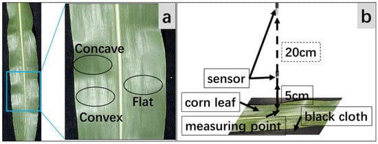
Figure 3.
Illustrations of different leaf curvatures (a) and measured heights (b).
From seven to fifteen days after inoculation, symptoms of southern corn rust appeared. Urediniums of Puccinia polysora were gradually generated on the leaf surface, and urediniospores were dispersed into the air after harvest. In this study, the SCR severity was classified into three levels based on the uredinium coverage by visual investigation.
Healthy: no uredinium on the surface (Figure 4a);
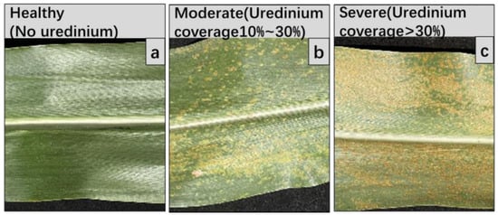
Figure 4.
Corn leaves of healthy (a), moderately infected (b) and severely infected (c) leaves.
Moderate: 10~30% was covered by urediniums (Figure 4b);
Severe: more than 30% was covered by urediniums (Figure 4c).
In this study, hyperspectral data were acquired from 25 August to 15 September 2021 with corn in the flowering stage. The measuring results were divided into 11 groups according to the differences in disease severity, measuring height and leaf curvature (Table 1).

Table 1.
Sample numbers under different measuring conditions.
Moreover, the hyperspectral data in Table 1 were combined into different datasets for further analysis. The sample numbers and samples contained in each dataset are shown in Table 2. The datasets are described in detail below.
Table 2.
Sample numbers and samples contained in different datasets.
Dataset (A): samples acquired under fully controlled conditions (measuring height = 5 cm; the target area was flat) to test the sensitivities of the different indices to the disease severity by ANOVA;
Dataset (B): samples acquired under partially controlled conditions (the measuring height varied; the target area was flat) to test the sensitivities of the different indices to the measuring height by ANOVA;
Dataset (C): samples acquired under partially controlled conditions (measuring height = 5 cm; the target area varied) to test the sensitivities of different indices to the leaf curvature by ANOVA;
Dataset (D): 66 mixed samples collected at different measuring heights to evaluate the separating capacities of different indices by random forest classification;
Dataset (E): 66 mixed samples collected with different leaf curvatures to evaluate the separating capacities of different indices by random forest classification;
Dataset (F): 66 mixed samples collected at different measuring heights and with different leaf curvatures to evaluate the separating capacities of different indices by random forest classification.
2.4. Data Preprocessing
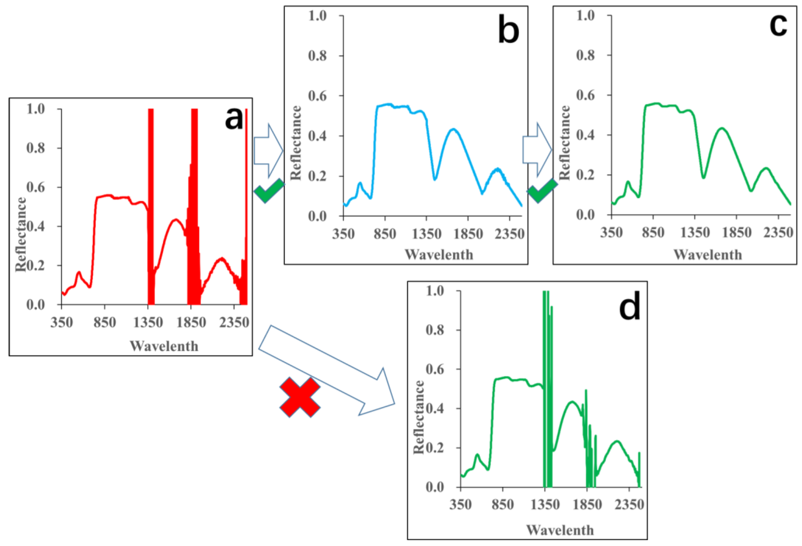
Due to the absorption of water vapor, the solar illumination signals in 1350~1430, 1800~2050 and 2300~2500 nm were weak, which resulted in fluctuations in the spectral curves (Figure 5a). Preprocessing was needed before data analysis. If Savitzky–Golay (SG) filtering [56] was used directly, the reflectance values at the wavelengths close to the fluctuation region would be filtered incorrectly (Figure 5d). In this study, a two-step preprocessing method was proposed: (1) a linear simulation was carried out to replace the abnormal values in the fluctuation ranges; and (2) SG filtering was applied afterwards.
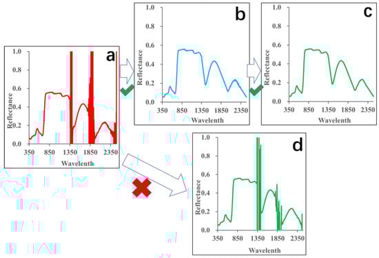
Figure 5.
Spectral curves of original data (a), linear simulation data (b), SG filtering data and (c,d) SG filtering data generated by one-step preprocessing.
The linear simulation procedure consisted of two steps: positioning the start and end wavelengths of the fluctuation region by using Equation (1), and generating simulating values based on a linear algorithm by using Equation (2) and replacing the original data (Figure 5b).
where is the reflectance at wavelength i. and are the reflectances at the start and end wavelengths of the fluctuation region, respectively. i, e and s are their corresponding wavelength values. As the linear simulated values in the fluctuation region were not actual data, they were not used for further analysis. In this study, SG filtering was carried out by using the scipy-signal function in Python 3.8. The SG filtering results are shown in Figure 5c.
2.5. Index Selection and Calculation
In this study, two SCR-specific and eight general stress-related indices were selected because these indices covered all the parts of the spectral region important for stress detection (i.e., the visible region, red-edge region, NIR and SWIR). The indices and their calculation formulas are listed in Table 3.
Table 3.
Indices selected for this study.
2.6. Data Analysis
2.6.1. Analysis of Variance
Analysis of variance (ANOVA), also known as the F test, is an important analysis tool. It splits an observed aggregate variability into two parts: systematic factors and random factors. The systematic factors have a statistical influence on the given dataset, while the random factors do not. In this study, ANOVA was conducted using R for Windows 4.1.2 with the essential packages (tidyverse, car and multcomp). Prior to conducting ANOVA, the homogeneity of the variance and normality of the reflectance distributions were tested.
2.6.2. Random Forest Classification
Random forest, a widely used classification algorithm, was proposed by Breiman [65]. Numerous decision trees are constructed, and the trees are split into many nodes. The Gini index is the internal parameter used to evaluate the importance of variables. In this study, a random forest classifier was employed using the sklearn package (version 0.23.2) in Python 3.8. The input samples were separated into two parts: the training dataset (70%) and test datasets (30%). Fifty duplicates were carried out for each classification process.
2.7. Evaluation of Classification Results
The classification results were evaluated in terms of the overall accuracy (OA), macro average of precision (MAP) and macro average of recall (MAR). The OA, MAP and MAR can be calculated by using Equations (3), (6) and (7), respectively.
where the TP (true positives), FP (false positives), TN (true negatives) and FN (false negatives) are four values computed based on the classification confusion matrix. n is the number of severities.
In this study, the OA, MAP and MAR were extracted from the accuracy reports provided by the classification_report function in the sklearn package (version 0.23.2).
3. Results
3.1. Spectral Characteristics of SCR-Infected Leaves
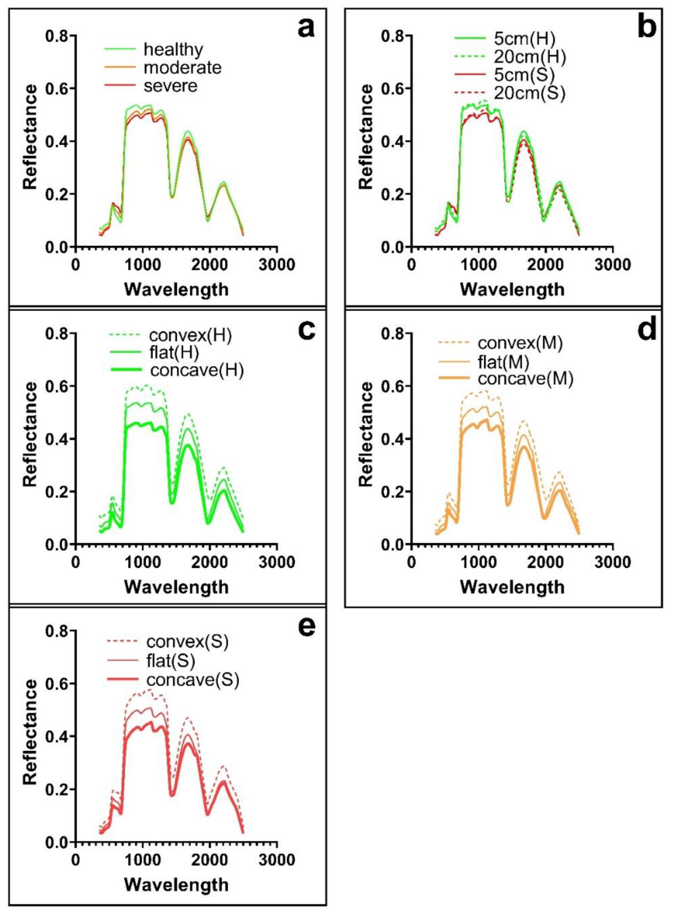
The hyperspectral data in Dataset (A) were averaged by group, and spectral curves were drawn based on the mean values of the reflectances (Figure 6a). It was observed that SCR infection resulted in noticeable changes in the spectral curves. The reflectance in the red (620~690 nm) range increased with an increase in disease severity, and an inverse relationship was exhibited for the blue (450~495 nm) range. Greater absorption could be observed in the NIR and SWIR ranges for the infected samples compared with the healthy leaves, and the more severe the disease, the more the leaf absorbed. In addition, crossings occurred in the red-edge range among spectral curves for different disease severities.
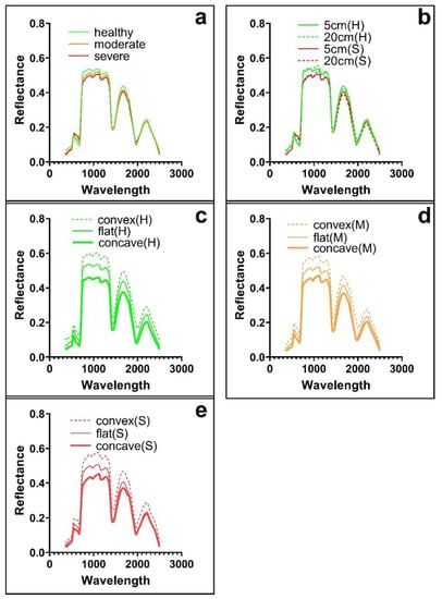
Figure 6.
Comparison of reflectances of corn leaves with different severities (a), different measuring heights (b) and different leaf curvatures (c–e). H, M and S in the legend denote healthy, moderate and severe, respectively.
Similarly, the spectra in Dataset (B) were also averaged by group, and the curves of the four groups are plotted in Figure 6b. For both healthy and severely infected leaves, the spectra measured at heights of 5 and 20 cm generally showed large similarity. Relative obvious differences in reflection could be observed at 1000~1150 and 1400~2500 nm. Larger differences between the healthy spectral curves (i.e., green solid line and green dotted line) and the severely infected curves (i.e., red solid line and red dotted line) could be observed. The spectra of the healthy leaves in the violet region showed a decreasing trend with an increase in measuring height.
The spectral curves for Dataset (C) are shown in Figure 6c–e. For healthy samples (green lines), shifts upward and downward were observed, respectively, with the leaf curvature changing from flat to convex and from flat to concave. Similar patterns were also observed for moderately infected and severely infected samples throughout the wavelength region.
3.2. Evaluation of Separating Capacity of Reflectance
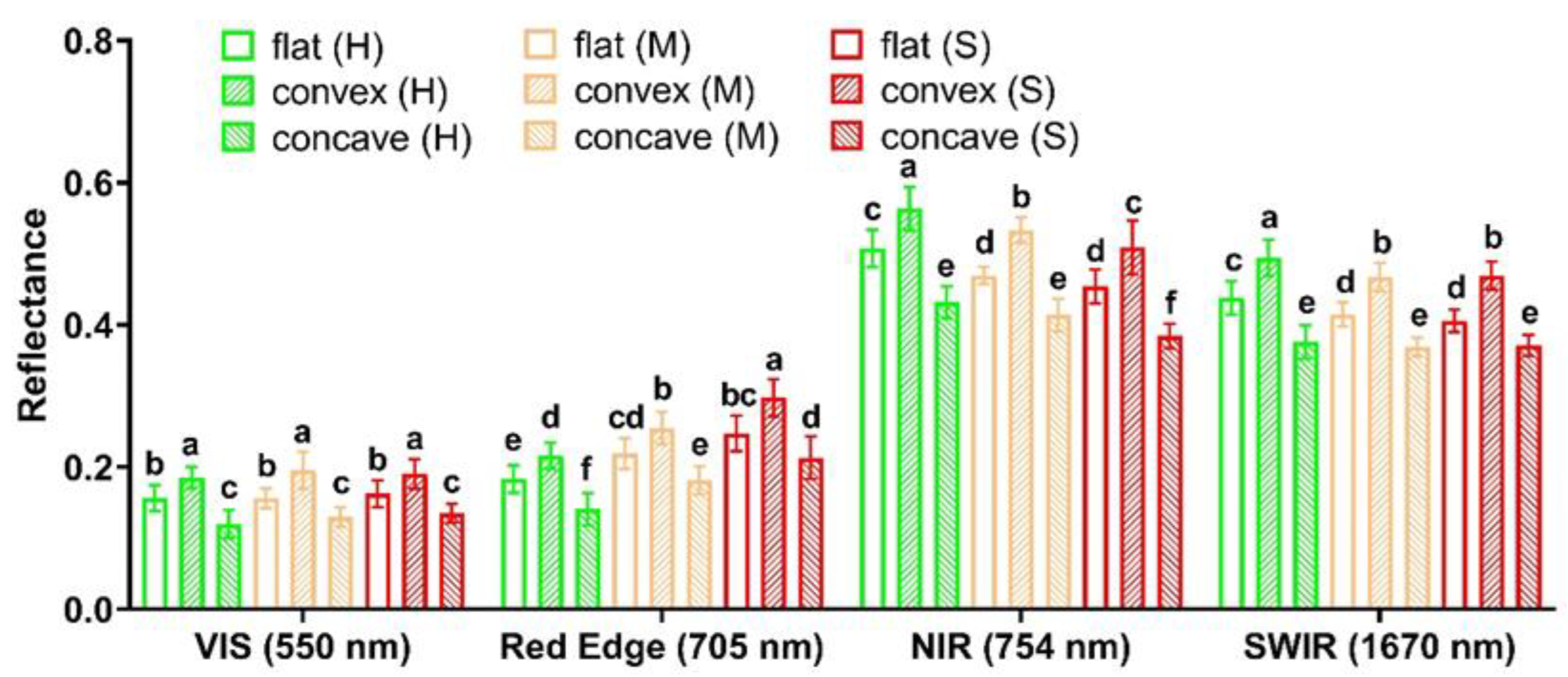
Four wavelengths (i.e., 550, 705, 754 and 1670 nm), which represented the typical spectral regions and composed the indices in Table 3, were selected. The reflectances at these four wavelengths in Dataset (C) were extracted. The mean value and standard deviation (SD) were calculated by group, and ANOVA was conducted afterwards (Figure 7). By comparing same-color histograms for each wavelength, we found that the reflectance values were sensitive to the leaf curvature. The values were always greater in convex areas and minor in concave areas regardless of the disease severity or spectral wavelength. The increase (or decrease) induced by the leaf curvature may counteract that induced by the disease severity. For example, the reflectance of the flat healthy sample was not significantly different from that of the concave moderately infected sample at 705 nm (both have the letter e in Figure 7). The lack of a significant difference between the reflectances of the flat healthy samples and convex severely infected samples at 754 nm is another example. Therefore, directly applying reflectance values for classification was not a reliable strategy.
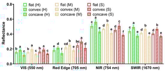
Figure 7.
Reflectance values in Dataset (C) at selected wavelengths. H, M and S in the legend denote healthy, moderate and severe, respectively. Error bar denotes standard deviation. Letters above histograms mark the significances, and values with the same letter are not significantly different.
3.3. Evaluation of Separating Capacity of Indices
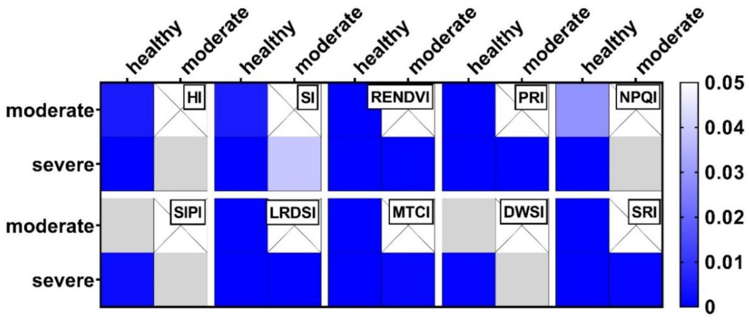
3.3.1. Most Indices Were Capable of Differentiating by Disease Severity
The index values were calculated by using the formulas in Table 3 based on the reflectance values in Dataset (A). An ANOVA test was conducted, and a heat map of the p values was plotted, as shown in Figure 8. No gray box existed in the sub-heatmap for the SI, RENDVI, PRI, LRDSI, MTCI and SRI, indicating their capabilities to differentiate between healthy, moderate and severe samples. Only healthy and infected samples could be identified by the HI and NPQI. The SIPI and DWSI, incapable of distinguishing healthy and moderate samples, performed the worst.
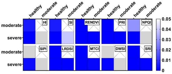
Figure 8.
Heat map of p values for different indices calculated based on Dataset (A). Cross means no data, and gray box means not significant.
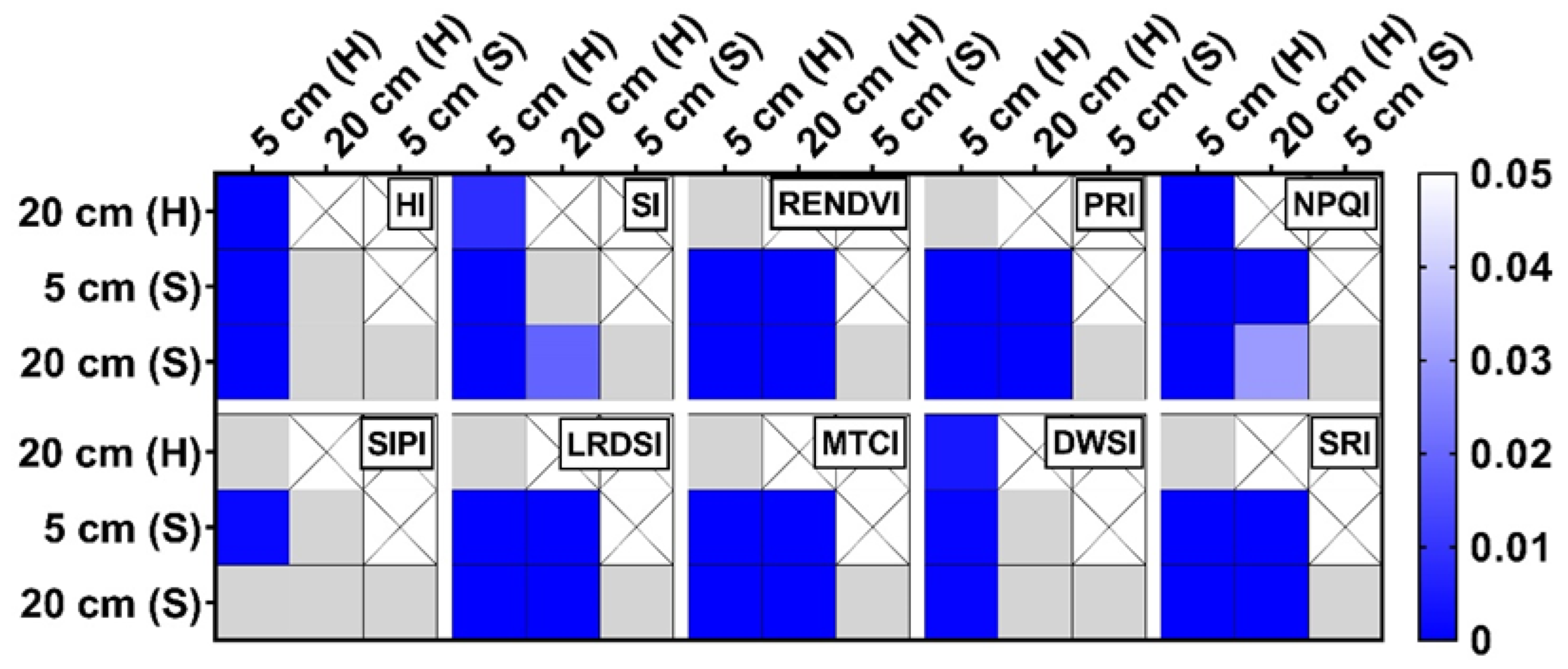
3.3.2. Half of the Indices Achieved Perfect Performance under Different Measuring Heights
The same processing as described in Section 3.3.1 was carried out based on the spectra in Dataset (B), and the heat map is shown in Figure 9. The RENDVI, PRI, LRDSI, MTCI and SRI achieved the best performance. The top-left and bottom-right gray boxes in the sub-heatmap of these indices revealed that the five best-performing indices were not sensitive to the measuring height, and the dark blue boxes indicated their capacities to separate healthy samples from severely infected samples at either measuring height. On the contrary, the HI, SI, NPQI and DWSI were sensitive to the measuring height, and none were capable of distinguishing between healthy and severely infected samples at the measuring height of 20 cm, except the NPQI.
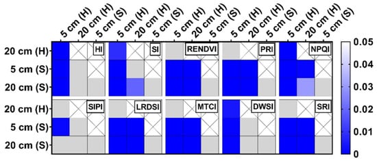
Figure 9.
Heat map of p values for different indices calculated based on Dataset (B). H, M and S in x and y axis denote healthy, moderate and severe, respectively. Cross means no data, and gray box means not significant.
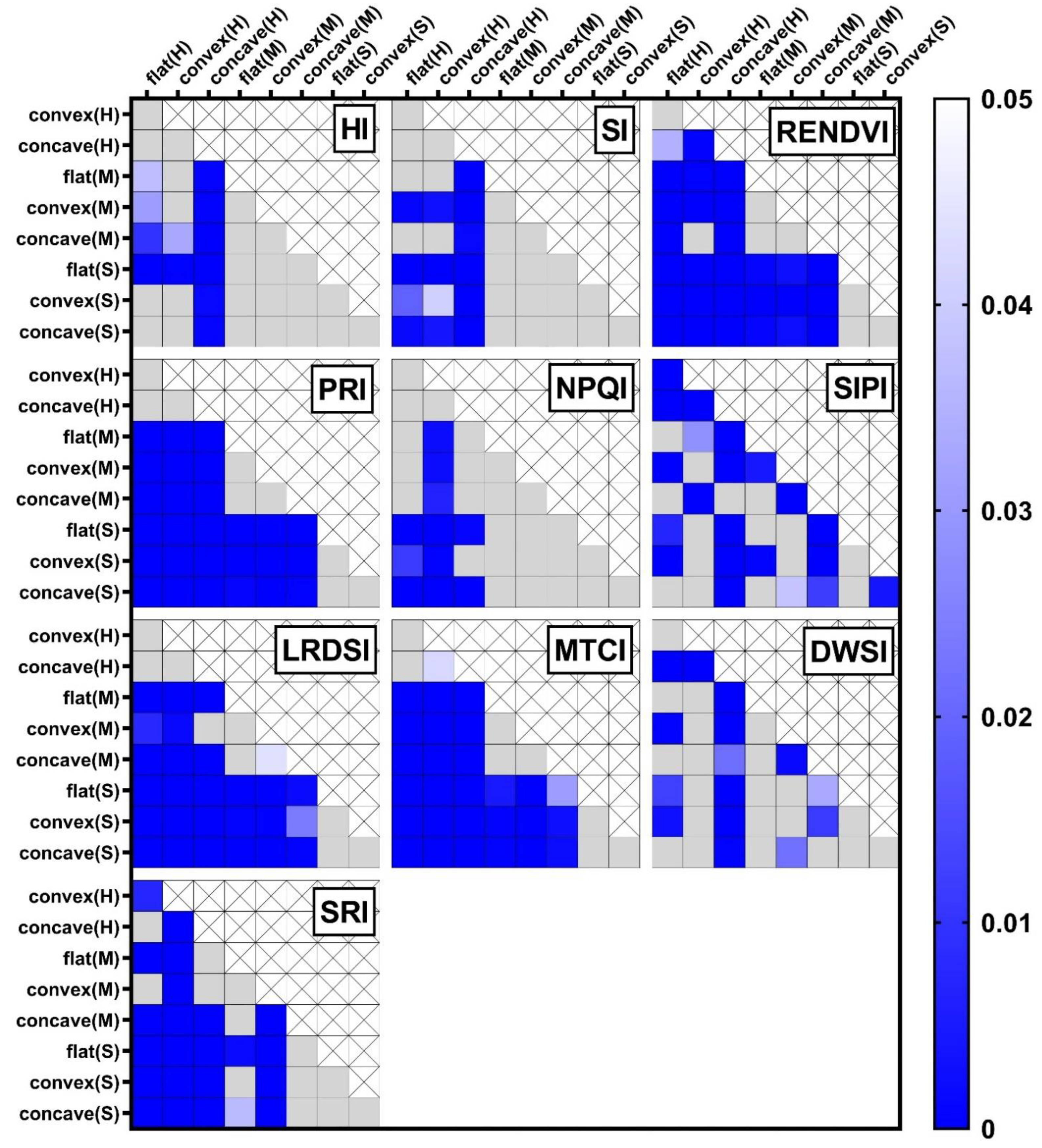
3.3.3. All indices Were Affected by Leaf Curvature to Varying Degrees except PRI
The same processing as described in Section 3.3.1 was carried out based on the spectra in Dataset (C), and the heat map is shown in Figure 10. The PRI outperformed all the other indices, as the PRI was not sensitive to the leaf curvature at any disease severity level (i.e., the nine gray boxes in the sub-heatmap for the PRI). Moreover, the disease severities could be identified perfectly by the PRI whether the leaves were flat or not (i.e., dark blue boxes in the sub-heatmap of the PRI). The RENDVI, LRDSI, MTCI and SRI achieved relatively good performance, while the other indices (i.e., the HI, SI, NPQI, SIPI and DWSI) were too affected by the leaf curvature.
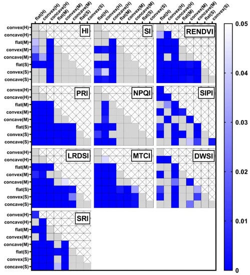
Figure 10.
Heat map of p values for different indices calculated based on Dataset (C). H, M and S in x and y axis denote healthy, moderate and severe, respectively. Cross means no data, and gray box means not significant.
3.4. Classification Accuracies Based on Different Indices
Based on the ANOVA test results, the SI, RENDVI, PRI, LRDSI, MTCI and SRI were selected for random forest classification. To avoid the impact of the imbalanced sample sizes on accuracy, Datasets (D–F) were constructed based on the same data framework (i.e., the numbers of healthy, moderately infected and severely infected samples were 30, 15 and 21, respectively) of Dataset (A). The random forest classifier was applied to Datasets (A and D–F), and the classification results are shown in Table 4.
Table 4.
OA, MAP and MAR values for different datasets based on single-index random forest classification. OA, MAP and MAR are overall accuracy, macro average of precision and macro average of recall, respectively. Maximum value of each parameter is highlighted in bold, and dataset details are described in Table 2.
In general, the RENDVI, PRI, LRDSI and MTCI performed better than the other two indices. The OA, MAP and MAR values varied from 37.41% to 82.00% with different datasets. For Dataset (A), in terms of the OA, the LRDSI ranked first with an overall accuracy of 82.00%, slightly above that of the PRI (80.60%), MTCI (80.40%) and RENDVI (78.70%), and well above that of the SI (61.00%) and SRI (71.00%). As for the MAP and MAR values, the MTCI performed the best, with accuracies of 78.34% and 77.91%, respectively, slightly above those of the LRDSI (78.01% and 77.16%), PRI (76.77% and 76.76%) and RENEVI (75.35% and 76.70%).
Although there were some special cases, a trend of a decline in accuracy was observed when the indices were applied to datasets consisting of mixed samples, and Dataset (F) showed the most significant drop in accuracy. The PRI was the only index that performed well across all the datasets, and the maximum OA, MAP and MAR values were observed for Datasets (D–F). The OA values for these datasets were 81.80%, 80.10% and 81.30%, respectively, and the MAP and MAR values ranged from 76.78% to 79.70%. Concerning both the robustness and accuracy, the PRI was regarded as the optimal index for SCR severity classification.
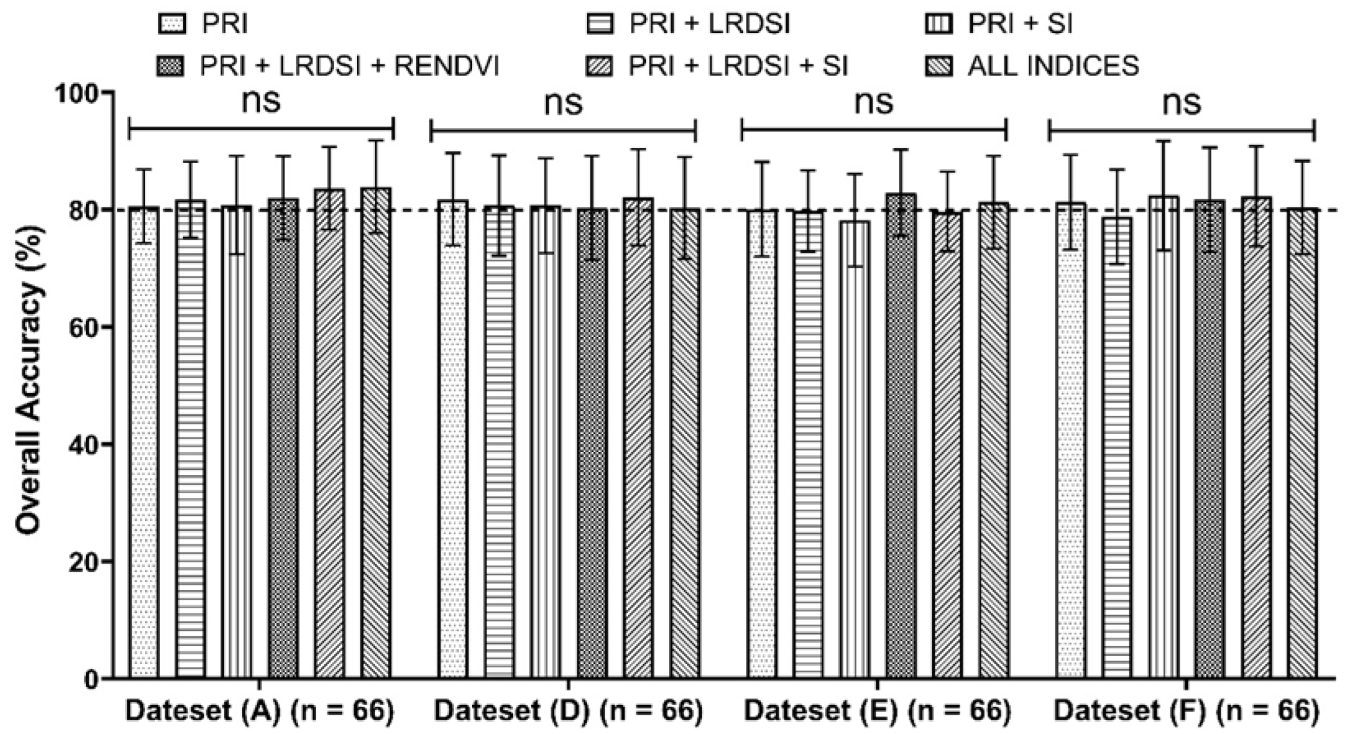
Finally, a series of multi-indices containing the PRI were combined, and the differences in the accuracy achieved with the single PRI and multi-indices were evaluated by ANOVA. The evaluation results are shown in Figure 11, which reveals that no significant difference between the performance of the single PRI and multi-indices for any dataset was observed.
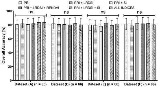
Figure 11.
Overall accuracies of random forest classification based on single PRI and multi-indices. Error bar denotes standard deviation. Dotted line means overall accuracy equals 80%, and ns above histograms means not significant. n in x axis means sample numbers, and dataset details are described in Table 2.
4. Discussion
Although leaf-level hyperspectral data have been applied for the detection of many stressors, such as disease [66], pests [67], water deficits [68] and nitrogen deficits [69], few articles have discussed the capability of the SCUSI with a full spectral range (350~2500 nm). Spectral data are affected by many factors under natural illumination, resulting in fluctuations, especially in the SWIR range, which have usually been avoided by using portable equipment with artificial illumination [48] or focusing on a limited spectral range (i.e., VIS–NIR) [50]. In this study, ANOVA was conducted to evaluate the sensitivities of indices to different severities, different measuring heights and different leaf curvatures on the basis of spectral signature analysis. Then, random forest classification was applied, and a single-index-based classification method was finally determined.
4.1. Analysis of Spectral Characteristics
The spectral curves in Figure 6a exhibit spectral features similar to those reported under artificial illumination conditions [22]. The reflectance of the SCR-infected sample increased in the red range, as this range is related to chlorophyll absorption. The invasion of Puccinia polysora destroyed the chlorophyll in mesophyll cells, and less light in the red range could be captured, resulting in higher reflectance values. The red edge was another region sensitive to stress [66]. The spectral curves of the SCR-infected samples had smaller slope values in the red-edge range, whereas the blue shift of the red edge [70] was not obvious. The growth of fungal hyphae changed the leaf’s inner structure, leading to a decrease in the reflectance of the infected leaves in the NIR range. With the development of the fungi, a water deficit gradually developed. The change in water content caused a decline in the reflectance in the SWIR region. The differences between the reflectance curves in Figure 6b were caused by compound factors such as the size of the coverage area and scattered light from surrounding objects. In fact, the difference in leaf curvature changed the incidence angle of the light. For the convex area, more light entered the sensor by specular reflection, and stronger signals were recorded by the equipment. On the contrary, the signal of the concave area relied more on diffuse reflection. This is why the convex area was brighter than the flat area, while the concave area was darker, as shown in Figure 3a. This can also explain why the reflectance values of the convex groups were greater than those of the other groups, as shown in Figure 6c–e and Figure 7.
4.2. Sensitivities of Reflectance and Indices under Different Measuring Conditions
The reflectance values were affected by many factors in the field under solar illumination. The difference induced by disease severity may be counteracted by other factors. For maize leaves, the leaf curvature was a factor that heavily influenced the reflectance values, and it can hardly be avoided, as the maize leaves were locally wrinkled. The high sensitivity of reflectance to the leaf curvature (Figure 7) reduced its suitability for disease severity monitoring. Constructing an index was a feasible solution, as the index contained more information than a single reflectance and increased the signal. For example, the NDVI is a wideband index that is commonly used, as it can increase vegetation signals and help to extract vegetation areas. Signals can also be increased for hyperspectral indices. Moreover, the division operation in index calculation can eliminate the influences of absolute reflectance values, leading to the result that the index is less sensitive to leaf curvature than reflectance.
The perfect performance of the six indices in Figure 8 demonstrated the effectiveness of those indices for the severity classifications. As most of the indices were proposed for detecting stresses other than SCR, the results also reveal their extensive suitability for similar stresses. The result for the HI is quite reasonable, as the HI was initially designed to differentiate between healthy and infected samples [22]. According to the ANOVA test results in Figure 9, all the indices can be used to differentiate between healthy and severely infected leaves at a measuring height of 5 cm, while the HI, SIPI and DWSI were incapable of distinguishing healthy samples from severely infected ones at a measuring height of 20 cm. Therefore, 5 cm was a reasonable measuring height for hyperspectral data collection. The high sensitivities of most of the indices to the leaf curvature are revealed in Figure 10, indicating that the leaf curvature had a broader impact than the measuring height. The perfect performance of the PRI according to all the ANOVA tests indicates its potential for classifying SCR severity.
4.3. Classification Accuracies of Single Indices and Multi-Indices
The results for the classification accuracies are consistent with the ANOVA test results. The PRI outperformed the other indices in terms of classification accuracy, and had the best performance according to the ANOVA test. The reflectance values of the healthy samples at 531 nm were greater than those of the infected samples, while a reverse trend occurred at 570 nm (Figure 6a). Moreover, the reflectance values in both bands were slightly affected by the measuring height (Figure 6b). Division was conducted to generate the PRI (Table 3), thus eliminating the effect of the leaf curvature. This may explain why the PRI performed so well. The performance of the RENDVI, LRDSI and MTCI was also acceptable, while the SI and SRI performed the worst, which also coincided with the ANOVA test results. Nevertheless, the classification accuracy contradicted the ANOVA test results in some cases. Despite the perfect ANOVA test result shown in Figure 9, the overall accuracy for Dataset (D) achieved by the RENDVI dropped from 78.70% to 67.10%, and this may be attributed to the different samples used for each test.
The conclusion that the PRI was effective for SCR classification is consist with that reported by Meng [22]. However, the accuracy achieved by the SI was only 61.80% for Dataset (A), lower than the reported 70.00% [22]. A possible reason for this discrepancy is that the reflectance values we measured in the SWIR region were not precise enough. It was noticeable that the differences among different-severity samples at around 1600 nm were not as significant as reported [22]. Although water vapor had little effect in 1500~1700 nm, the solar radiance in this range was much weaker (under 0.05 w/m2/nm/sr) than the radiance (above 0.1 w/m2/nm/sr) of artificial illumination [55]. As the hyperspectral data in this study were collected under solar illumination, slight differences in the signal at around 1600 nm were not captured by the sensor, and thus, the reflectance was less reliable than that obtained under artificial illumination. This can explain why all the indices containing SWIR bands (i.e., the HI, SI and DWSI) showed poorer performance in this study; therefore, equipment with artificial illumination is indispensable if the target index contains SWIR bands. The poor performance of the NPQI and SRI may have been caused by the bands that composed these indices. The bands were located in a very narrow spectral range, which reduced the capacities of the indices to increase signals. The reason for the bad performance of the SIPI may be that the SIPI was mainly used at the canopy level.
The similar performance among the single PRI and multi-indices in Figure 11 demonstrate that combining more indices may not improve the accuracy, and this may be attributed to the effect of data redundancy.
4.4. Future Study
As only healthy and severely infected samples were discussed in Section 3.3.2, the ANOVA test results may have changed if moderately infected samples measured at a height of 20 cm had been added. Samples under more complex conditions, such as measuring convex or concave areas at a measuring height of 20 cm, will be collected and analyzed in our future study. As only measuring heights of 5 and 20 cm were addressed in this study, there may be a measuring height better than 5 cm that could be determined if more gradients of measuring heights were designed. Other more sophisticated indices were not discussed in this study, as we aimed to determine an easy, rapid and reliable indicator for SCR classification. Other factors, such as the maize variety, growing stage and leaf location, were not addressed either; a wider dataset containing spectra collected under more sophisticated conditions will be necessary in a future study.
The identification of disease or classification of the disease severity in the symptom appearance phase is of very limited help for disease control. Based on the results in this study, the PRI should be applied for SCR identification in the incubation phase. Moreover, regional SCR monitoring is more practical, and the relatively good performance of the RENDVI indicates potential for SCR identification based on UAV and satellite images. Satellites such as Sentinel-2 [24] and GF-6 (gaofen-6, a Chinese satellite launched in 2018) have double red-edge bands, and the wideband RENDVI can be easily calculated. Hence, UAV and satellite images are expected to be applied for the identification of SCR at a regional scale in the future. Other stresses, such as water deficiency, nutrient deficiency, pests or other diseases, may cause the same differences in reflectance. A comparative study considering other stresses was, therefore, considered worth performing. Among all the stresses, the detection of common corn rust (CCR) caused by Puccinia sorghi would be most valuable, as SCR and CCR both infect maize, and the symptoms are too similar to be differentiated by visual interpretation. A precise but costly method for the identification of SCR and CCR is molecular-based detection. An easier but hazardous method is observing the shapes of urediniospores soaked in 95% sulfuric acid or 75% hydrochloric acid [71]. It would be helpful for agricultural practice if a safe, rapid and easy detection method was proposed. As detection models for different rusts affecting wheat have been proposed [50], an index-based detection method for SCR and CCR will very likely be achieved.
5. Conclusions
In this study, different groups of SCUSI were collected. Ten candidate indices were calculated based on the SCUSI, and their sensitivities to the disease severity, measuring height and leaf curvature were evaluated by ANOVA tests. The six better-performing indices according to the ANOVA tests were applied to a random forest classifier, and the optimal index was finally determined.
The study demonstrates that (1) indices are more reliable for SCR severity classification than reflectances; (2) collecting the SCUSI at a measuring height of 5 cm is a better choice; (3) the PRI is the optimal index for classifying SCR severity, and the overall accuracy can reach 81.30% for mixed samples; (4) compared with the PRI alone, multi-indices cannot significantly improve the classification accuracy; and (5) if an index with a SWIR-range wavelength is selected as the indicator for disease detection, using equipment with artificial illumination is the optimal option.
The PRI was determined to be the optimal index for SCR detection in this study, laying the foundation for detecting SCR during the incubation period and performing a comparative study for SCR and CCR.
Author Contributions
Conceptualization, J.G. and Z.M.; methodology, J.G.; formal analysis, J.G. and M.D.; writing—original draft preparation, J.G. and Q.S.; writing—review and editing, J.G., Q.S., M.D., J.D., H.W. and Z.M.; funding acquisition, Z.M. All authors have read and agreed to the published version of the manuscript.
Funding
This work was supported by the Natural Science Foundation of China (grant 31972211).
Acknowledgments
We would like to thank Limin Wang and Fugang Yang in CAAS (Chinese Academy of Agricultural Science) for the professional guidance on the use of instruments.
Conflicts of Interest
The authors declare no conflict of interest.
References
- FAO. FAOSTAT-Agriculture, Food and Agricultural Organizations of the United Nations. 2019. Available online: http://faostat3.fao.org/brpwse/Q/QC/E (accessed on 19 July 2021).
- Wang, Y.Q.; Gao, F.; Gao, G.Y.; Zhao, J.Y.; Wang, X.G.; Zhang, R. Production and cultivated area variation in cereal, rice, wheat and maize in China (1998–2016). Agronomy 2019, 9, 222. [Google Scholar] [CrossRef] [Green Version]
- Ali, M.M.; Bachik, N.A.; Muhadi, N.A.; Yusof, T.N.T.; Gomes, C. Non-destructive techniques of detecting plant diseases: A review. Physiol. Mol. Plant Pathol. 2019, 108, 101426–101437. [Google Scholar] [CrossRef]
- Sun, Q.Y.; Li, L.F.; Guo, F.F.; Zhang, K.Y.; Dong, J.Y.; Luo, Y.; Ma, Z.H. Southern corn rust caused by Puccinia polysora Underw.: A review. Phytopathol. Res. 2021, 3, 25. [Google Scholar] [CrossRef]
- Sun, Q.Y.; Liu, J.; Zhang, K.Y.; Huang, C.; Li, L.F.; Dong, J.Y.; Luo, Y.; Ma, Z.H. De novo transcriptome assembly, polymorphic SSR markers development and population genetics analyses for southern corn rust (Puccinia polysora). Sci. Rep. 2021, 11, 18029. [Google Scholar] [CrossRef] [PubMed]
- Yan, J.H.; Luo, Y.; Chen, T.T.; Huang, C.; Ma, Z.H. Field distribution of wheat stripe rust latent infection using real-time PCR. Plant Dis. 2012, 96, 544–551. [Google Scholar] [CrossRef] [Green Version]
- Bohnenkamp, D.; Kuska, M.T.; Mahlein, A.K.; Behmann, J. Hyperspectral signal decomposition and symptom detection of wheat rust disease at the leaf scale using pure fungal spore spectra as reference. Plant Pathol. 2019, 68, 1188–1195. [Google Scholar] [CrossRef]
- Hunt, E.R.; Rock, B.N. Detection of changes in leaf water-content using near-infrared and middle-infrared reflectances. Remote Sens. Environ. 1989, 30, 43–54. [Google Scholar]
- Cheng, T.; Rivard, B.; Sanchez-Azofeifa, A. Spectroscopic determination of leaf water content using continuous wavelet analysis. Remote Sens. Environ. 2011, 115, 659–670. [Google Scholar] [CrossRef]
- Thomas, S.; Kuska, M.T.; Bohnenkamp, D.; Brugger, A.; Alisaac, E.; Wahabzada, M.; Behmann, J.; Mahlein, A.K. Benefits of hyperspectral imaging for plant disease detection and plant protection: A technical perspective. J. Plant Dis. Prot. 2017, 125, 5–20. [Google Scholar] [CrossRef]
- Visible Light Definition and Wavelengths. Available online: https://www.thoughtco.com/definition-of-visible-light-605941 (accessed on 10 May 2022).
- Smith, K.L.; Steven, M.D.; Colls, J.J. Use of hyperspectral derivative ratios in the red-edge region to identify plant stress responses to gas leaks. Remote Sens. Environ. 2004, 92, 207–217. [Google Scholar] [CrossRef]
- Lowe, A.; Harrison, N.; French, A.P. Hyperspectral image analysis techniques for the detection and classification of the early onset of plant disease and stress. Plant Methods 2017, 13, 80. [Google Scholar] [CrossRef] [PubMed]
- Filella, I.; Penuelas, J. The red edge position and shape as indicators of plant chlorophyll content, biomass and hydric status. Int. J. Remote Sens. 1994, 15, 1459–1470. [Google Scholar] [CrossRef]
- Oerke, E.C.; Herzog, K.; Toepfer, R. Hyperspectral phenotyping of the reaction of grapevine genotypes to Plasmopara viticola. J. Exp. Bot. 2016, 67, 5529–5543. [Google Scholar] [CrossRef] [PubMed] [Green Version]
- Robnik-Šikonja, M.; Kononenko, I. Theoretical and empirical analysis of relief and rrelieff. Mach. Learn. 2003, 53, 23–69. [Google Scholar] [CrossRef] [Green Version]
- Adam, E.; Deng, H.T.; Odindi, J.; Abdel-Rahman, E.M.; Mutanga, O. Detecting the early stage of phaeosphaeria leaf spot infestations in maize crop using in-situ hyperspectral data and guided regularized random forest algorithm. J. Spectros. 2017, 2017, 6961387. [Google Scholar] [CrossRef]
- Golhani, K.; Balasundram, S.K.; Vadamalai, G.; Pradhan, B. A review of neural networks in plant disease detection using hyperspectral data. Inf. Process. Agric. 2018, 5, 354–371. [Google Scholar] [CrossRef]
- Wang, L.M.; Liu, J.; Shao, J.; Yang, F.G.; Gao, J.M. Remote sensing index selection of leaf blight disease in spring maize based on hyperspectral data. Trans. Chin. Soc. Agric. Eng. 2017, 33, 170–177, (In Chinese with English Abstract). [Google Scholar]
- Shi, Y.; Huang, W.J.; Gonzalez-Moreno, P.; Luke, B.; Dong, Y.Y.; Zheng, Q.; Ma, H.Q.; Liu, L.Y. Wavelet-based rust spectral feature set (WRSFs): A novel spectral feature set based on continuous wavelet transformation for tracking progressive host-pathogen interaction of yellow rust on wheat. Remote Sens. 2018, 10, 525. [Google Scholar] [CrossRef] [Green Version]
- Zhang, N.; Yang, G.J.; Pan, Y.C.; Yang, X.D.; Chen, L.P.; Zhao, C.J. A review of advanced technologies and development for hyperspectral-based plant disease detection in the past three decades. Remote Sens. 2020, 12, 3188. [Google Scholar] [CrossRef]
- Meng, R.; Lv, Z.G.; Yan, J.B.; Chen, G.S.; Zhao, F.; Zeng, L.L.; Xu, B.Y. Development of spectral disease indices for southern corn rust detection and severity classification. Remote Sens. 2020, 12, 3233. [Google Scholar] [CrossRef]
- Skoneczny, H.; Kubiak, K.; Spiralski, M.; Kotlarz, J. Fire blight disease detection for apple trees: Hyperspectral analysis of healthy, infected and dry leaves. Remote Sens. 2020, 12, 2101. [Google Scholar] [CrossRef]
- Dhau, I.; Adam, E.; Mutanga, O.; Ayisi, K.; Abdel-Rahman, E.M.; Odindi, J.; Masocha, M. Testing the capability of spectral resolution of the new multispectral sensors on detecting the severity of grey leaf spot disease in maize crop. Geocarto Int. 2018, 33, 1223–1236. [Google Scholar] [CrossRef]
- Xie, C.; Yang, C.; He, Y. Hyperspectral imaging for classification of healthy and gray mold diseased tomato leaves with different infection severities. Comput. Electron. Agric. 2017, 135, 154–162. [Google Scholar] [CrossRef]
- Ashourloo, D.; Aghighi, H.; Matkan, A.A.; Mobasheri, M.R.; Rad, A.M. An investigation into machine learning regression techniques for the leaf rust disease detection using hyperspectral measurement. IEEE J. Sel. Top. Appl. Earth Obs. Remote Sens. 2016, 9, 4344–4351. [Google Scholar] [CrossRef]
- Sarhadi, A.; Burn, D.H.; Johnson, F.; Mehrotra, R.; Sharma, A. Water resources climate change projections using supervised nonlinear and multivariate soft computing techniques. J. Hydrol. 2016, 536, 119–132. [Google Scholar] [CrossRef] [Green Version]
- Congalton, R.G. A review of assessing the accuracy of classifications of remotely sensed data. Remote Sens. Environ. 1991, 37, 35–46. [Google Scholar] [CrossRef]
- Sklearn.Metrics.Precision_Recall_Fscore_Support. Available online: https://scikit-learn.org/stable/modules/generated/sklearn.metrics.precision_recall_fscore_support.html (accessed on 10 May 2022).
- Lama, G.F.C.; Sadeghifar, T.; Azad, M.T.; Sihag, P.; Kisi, O. On the indirect estimation of wind wave heights over the southern coasts of Caspian Sea: A comparative analysis. Water 2022, 14, 843. [Google Scholar] [CrossRef]
- Albarracín, J.F.H.; Oliveira, R.S.; Hirota, M.; DosSantos, J.A.; Torres, R.D.S. A soft computing approach for selecting and combining spectral bands. Remote Sens. 2020, 12, 2267. [Google Scholar] [CrossRef]
- Li, H.; Xiao, G.G.; Xia, T.; Tang, Y.Y.; Li, L.Q. Hyperspectral image classification using functional data analysis. IEEE Trans. Cybern. 2014, 44, 1544–1555. [Google Scholar]
- Sadeghifar, T.; Lama, G.F.C.; Sihag, P.; Bayram, A.; Kisi, O. Wave height predictions in complex sea flows through soft-computing models: Case study of Persian Gulf. Ocean. Eng. 2022, 245, 110467. [Google Scholar] [CrossRef]
- Yang, S.B.; Xia, T.L.; Zhang, Z.Q.; Zheng, C.W.; Li, X.F.; Li, H.Y.; Xu, J.J. Prediction of significant wave heights based on CS-BP model in the South China Sea. IEEE Access 2019, 7, 147490–147500. [Google Scholar] [CrossRef]
- Pham, Q.B.; Mohammadpour, R.; Linh, N.T.T.; Mohajane, M.; Pourjasem, A.; Sammen, S.S.; Anh, D.T.; Nam, V.T. Application of soft computing to predict water quality in wetland. Environ. Sci. Pollut. Res. 2021, 28, 185–200. [Google Scholar] [CrossRef] [PubMed]
- Arabameri, A.; Blaschke, T.; Pradhan, B.; Pourghasemi, H.R.; Tiefenbacher, J.P.; Bui, D.T. Evaluation of recent advanced soft computing techniques for gully erosion susceptibility mapping: A Comparative Study. Sensors 2020, 20, 335. [Google Scholar] [CrossRef] [PubMed] [Green Version]
- Hong, H.Y.; Kornejady, A.; Soltani, A.; Termeh, S.V.R.; Liu, J.Z.; Zhu, A.X.; Hesar, A.Y.; Bin Ahmad, B.; Wang, Y. Landslide susceptibility assessment in the Anfu County, China: Comparing different statistical and probabilistic models considering the new topo-hydrological factor (HAND). Earth Sci. Inform. 2018, 11, 605–622. [Google Scholar] [CrossRef]
- Esposito, M.; Crimaldi, M.; Cirillo, V.; Sarghini, F.; Maggio, A. Drone and sensor technology for sustainable weed management: A review. Chem. Biol. Technol. Agric. 2021, 8, 18. [Google Scholar] [CrossRef]
- Dal-Sasso, S.F.; Pizarro, A.; Samela, C.; Mita, L.; Manfreda, S. Exploring the optimal experimental setup for surface flow velocity measurements using PTV. Environ. Monit. Assess. 2018, 190, 460. [Google Scholar] [CrossRef]
- Tian, L.; Xue, B.W.; Wang, Z.Y.; Li, D.; Yao, X.; Cao, Q.; Zhu, Y.; Cao, W.X.; Cheng, T. Spectroscopic detection of rice leaf blast infection from asymptomatic to mild stages with integrated machine learning and feature selection. Remote Sens. Environ. 2021, 257, 112350. [Google Scholar] [CrossRef]
- Zhang, J.C.; Pu, R.L.; Wang, J.H.; Huang, W.J.; Yuan, L.; Luo, J.H. Detecting powdery mildew of winter wheat using leaf level hyperspectral measurements. Comput. Electron. Agric. 2012, 85, 13–23. [Google Scholar] [CrossRef]
- Appeltans, S.; Guerrero, A.; Nawar, S.; Pieters, J.; Mouazen, A.M. Practical recommendations for hyperspectral and thermal proximal disease sensing in potato and leek fields. Remote Sens. 2020, 12, 1939. [Google Scholar] [CrossRef]
- Garhwal, A.S.; Pullanagari, R.R.; Li, M.; Reis, M.M.; Archer, R. Hyperspectral imaging for identification of zebra chip disease in potatoes. Biosyst. Eng. 2020, 197, 306–317. [Google Scholar] [CrossRef]
- Chen, T.T.; Zhang, J.L.; Chen, Y.; Wan, S.B.; Zhang, L. Detection of peanut leaf spots disease using canopy hyperspectral reflectance. Comput. Electron. Agric. 2019, 156, 677–683. [Google Scholar] [CrossRef]
- Herrmann, I.; Vosberg, S.K.; Ravindran, P.; Singh, A.; Chang, H.X.; Chilvers, M.I.; Conley, S.P.; Townsend, P.A. Leaf and canopy level detection of fusarium virguliforme (sudden death syndrome) in soybean. Remote Sens. 2018, 10, 426. [Google Scholar] [CrossRef] [Green Version]
- Moshou, D.; Bravo, C.; West, J.; Wahlen, T.; McCartney, A.; Ramon, H. Automatic detection of ‘yellow rust’ in wheat using reflectance measurements and neural networks. Comput. Electron. Agric. 2004, 44, 173–188. [Google Scholar] [CrossRef]
- Yao, Z.F.; Lei, Y.; He, D.J. Early visual detection of wheat stripe rust using visible/near-infrared hyperspectral imaging. Sensors 2019, 19, 952. [Google Scholar] [CrossRef] [PubMed] [Green Version]
- Zhao, J.L.; Huang, L.S.; Huang, W.J.; Zhang, D.Y.; Yuan, L.; Zhang, J.C.; Liang, D. Hyperspectral measurements of severity of stripe rust on individual wheat leaves. Eur. J. Plant Pathol. 2014, 139, 401–411. [Google Scholar] [CrossRef]
- Liu, Q.; Gu, Y.L.; Wang, S.H.; Wang, C.C.; Ma, Z.H. Canopy spectral characterization of wheat stripe rust in latent period. J. Spectrosc. 2015, 2015, 126090. [Google Scholar] [CrossRef] [Green Version]
- Wang, H.; Qin, F.; Ruan, L.; Wang, R.; Liu, Q.; Ma, Z.H.; Li, X.L.; Cheng, P.; Wang, H.G. Identification and severity determination of wheat stripe rust and wheat leaf rust based on hyperspectral data acquired using a black-paper-based measuring method. PLoS ONE 2016, 11, e0154648. [Google Scholar] [CrossRef]
- Dehkordi, R.H.; El Jarroudi, M.; Kouadio, L.; Meersmans, J.; Beyer, M. Monitoring wheat leaf rust and stripe rust in winter wheat using high-resolution UAV-based red-green-blue imagery. Remote Sens. 2020, 12, 3696. [Google Scholar] [CrossRef]
- Ruan, C.; Dong, Y.Y.; Huang, W.J.; Huang, L.S.; Ye, H.C.; Ma, H.Q.; Guo, A.T.; Ren, Y. Prediction of wheat stripe rust occurrence with time series sentinel-2 images. Agriculture 2021, 11, 1079. [Google Scholar] [CrossRef]
- Xu, J.; Miao, T.; Zhou, Y.C.; Xiao, Y.; Deng, H.B.; Song, P.; Song, K. Classification of maize leaf diseases based on hyperspectral imaging technology. J. Opt. Technol. 2020, 87, 212–217. [Google Scholar] [CrossRef]
- Luo, L.L.; Chang, Q.R.; Wang, Q.; Huang, Y. Identification and severity monitoring of maize dwarf mosaic virus infection based on hyperspectral measurements. Remote Sens. 2021, 13, 4560. [Google Scholar] [CrossRef]
- Analytical Spectral Devices, Inc. (ASD). Technical Guide, 3rd ed.; Analytical Spectral Devices, Inc.: Boulder, CO, USA, 1999; Available online: https://wiki.chem.gwu.edu/MillerLab/images/3/3e/FieldSpecTechGuide.pdf (accessed on 10 May 2022).
- Schafer, R.W. What is a savitzky-golay filter? IEEE Signal Process. Mag. 2011, 28, 111–117. [Google Scholar] [CrossRef]
- Evangelides, C.; Nobajas, A. Red-edge normalised difference vegetation index (NDVI705) from sentinel-2 imagery to assess post-fire regeneration. Remote Sens. Appl. Soc. Environ. 2020, 17, 100283. [Google Scholar] [CrossRef]
- Gamon, J.A.; Penuelas, J.; Field, C.B. A narrow-waveband spectral index that tracks diurnal changes in photosynthetic efficiency. Remote Sens. Environ. 1992, 41, 35–44. [Google Scholar] [CrossRef]
- Uelas, J.P.; Filella, I.; Lloret, P.; Oz, F.M.; Vilajeliu, M. Reflectance assessment of mite effects on apple trees. Int. J. Remote Sens. 1995, 16, 2727–2733. [Google Scholar]
- Penuelas, J.; Baret, F.; Filella, I. Semi empirical indexes to assess carotenoids chlorophyll-a ratio from leaf spectral reflectance. Photosynthetica 1995, 31, 221–230. [Google Scholar]
- Ashourloo, D.; Mobasheri, M.R.; Huete, A. Developing two spectral disease indices for detection of wheat leaf rust (Pucciniatriticina). Remote Sens. 2014, 6, 4723–4740. [Google Scholar] [CrossRef] [Green Version]
- Dash, J.; Curran, P.J. The MERIS terrestrial chlorophyll index. Int. J. Remote Sens. 2004, 25, 5403–5413. [Google Scholar] [CrossRef]
- Apan, A.; Held, A.; Phinn, S.; Markley, J. Detecting sugarcane ‘orange rust’ disease using EO-1 hyperion hyperspectral imagery. Int. J. Remote Sens. 2004, 25, 489–498. [Google Scholar] [CrossRef] [Green Version]
- Hernández-Clemente, R.; Navarro-Cerrillo, R.M.; Zarco-Tejada, P.J. Carotenoid content estimation in a heterogeneous conifer forest using narrow-band indices and PROSPECT+DART simulations. Remote Sens. Environ. 2012, 127, 298–315. [Google Scholar] [CrossRef]
- Breiman, L. Random forests. Mach. Learn. 2001, 45, 5–32. [Google Scholar] [CrossRef] [Green Version]
- Mahlein, A.K.; Rumpf, T.; Welke, P.; Dehne, H.W.; Plümer, L.; Steiner, U.; Oerke, E.C. Development of spectral indices for detecting and identifying plant diseases. Remote Sens. Environ. 2013, 128, 21–30. [Google Scholar] [CrossRef]
- Furuya, D.E.G.; Ma, L.F.; Pinheiro, M.M.F.; Gomes, F.D.G.; Goncalvez, W.N.; Marcato, J.; Rodrigues, D.D.; Blassioli-Moraes, M.C.; Michereff, M.F.F.; Borges, M.; et al. Prediction of insect-herbivory-damage and insect-type attack in maize plants using hyperspectral data. Int. J. Appl. Earth Obs. Geoinf. 2021, 105, 102608. [Google Scholar]
- Krishna, G.; Sahoo, R.N.; Singh, P.; Bajpai, V.; Patra, H.; Kumar, S.; Dandapani, R.; Gupta, V.K.; Viswanathan, C.; Ahmad, T.; et al. Comparison of various modelling approaches for water deficit stress monitoring in rice crop through hyperspectral remote sensing. Agric. Water Manag. 2019, 213, 231–244. [Google Scholar] [CrossRef]
- Devadas, R.; Lamb, D.W.; Backhouse, D.; Simpfendorfer, S. Sequential application of hyperspectral indices for delineation of stripe rust infection and nitrogen deficiency in wheat. Precis. Agric. 2015, 16, 477–491. [Google Scholar] [CrossRef] [Green Version]
- Carter, G.A.; Miller, R.L. Early detection of plant stress by digital imaging within narrow stress-sensitive wavebands. Remote Sens. Environ. 1994, 50, 295–302. [Google Scholar] [CrossRef]
- Huang, L.Q.; Zhang, K.Y.; Dong, J.Y.; Sun, Q.Y.; Li, L.F.; Ma, Z.H. A fast method for distinguishing southern rust pathogen Puccinia polysora from common rust pathogen Puccinia sorghi. J. Plant Prot. 2020, 47, 1385–1386. (In Chinese) [Google Scholar]

Publisher’s Note: MDPI stays neutral with regard to jurisdictional claims in published maps and institutional affiliations. |
© 2022 by the authors. Licensee MDPI, Basel, Switzerland. This article is an open access article distributed under the terms and conditions of the Creative Commons Attribution (CC BY) license (https://creativecommons.org/licenses/by/4.0/).