Abstract
Forest above-ground biomass (AGB) is an important index to evaluate forest carbon sequestration capacity, which is very important to maintain the stability of forest ecosystems. At present, the wide use of remote sensing technology makes it possible to estimate the large-scale forest AGB accurately and efficiently. Airborne hyperspectral remote sensing data can obtain rich spectral information and spatial structure information on the forest canopy with the characteristics of high spatial and hyperspectral resolution. Airborne LiDAR data can describe the three-dimensional structure characteristics of a forest and provide vertical structure information related to biomass. Based on the characteristics of the two data sources, this study takes Gaofeng forest farm in Nanning, Guangxi, as the study area, Chinese fir, pine tree, eucalyptus and other broadleaved trees as the research object, and constructs the AGB estimation models of different tree species by fusing airborne LiDAR and hyperspectral features. Firstly, spectral features, texture features, vegetation index, wavelet transform features and edge features are extracted from hyperspectral data. Canopy structure features, point cloud structure features, point cloud density features and terrain features are extracted from airborne LiDAR data. Secondly, the random forest (RF) method is used to screen the features of the two sets of data, and the features with the highest importance are selected. Finally, based on the optimal features of the two data sources, the forest AGB model is constructed using the multiple stepwise regression method. The results show that the texture features extracted by wavelet transform can be used for AGB modeling. The AGB of eucalyptus has high correlation with height features derived from airborne LiDAR, the AGB of other broadleaved trees mostly depends on the wavelet transform texture features from airborne hyperspectral data, while the AGB of Chinese fir and pine tree has high correlation with both height features and spectral features. Feature-fusion-based LiDAR and hyperspectral data can greatly improve the accuracy of the AGB models. The accuracy of the optimal AGB models of Chinese fir, pine tree, eucalyptus and other broadleaved trees is 0.78, 0.95, 0.72 and 0.89, respectively. In conclusion, more accurate estimation results can be obtained by combining active and passive remote sensing data for forest AGB estimation, which provides a solution for carbon storage assessment and forest ecosystem assessment.
1. Introduction
Forests are important natural resources for maintaining ecological balance and stability. The changes in forest resources and reserves will directly affect the decisions of major national forestry planning [1]. At the same time, as a natural and renewable resource, the quantity and quality of forests will directly affect national economic construction and people’s quality of life [2]. In 2007, a report from the IPCC (United Nations Intergovernmental Panel on Climate Change) pointed out that forestry has multiple benefits and has the dual functions of mitigating and adapting to climate change. This report is an economic and effective measure to increase carbon sequestration and reduce emissions in the next 30–50 years. The Paris Agreement also lists the forestry provisions separately, encourages countries to take actions to protect and enhance forest carbon pools and sinks after 2020, and continues to encourage developing countries to implement and support REDD+ (reducing deforestation, mitigating forest degradation and reducing greenhouse gas emissions). China also put forward the vision of “carbon peaking and carbon neutralization” in 2020, which shows that forest resources play an important role in global climate change and ecological balance. Therefore, it is necessary to monitor and assess the dynamic information of forest resources in time.
China is rich in forest resources and various forest types, which occupy an important position in the terrestrial ecosystem. At the same time, the forest community structure is complex and the biomass is high. More than 80% of the forest vegetation biomass is stored in the ecosystem. Therefore, the study of forest biomass estimation can better evaluate the problems of forest productivity and forest carbon cycle, and provide key data support for the study of global climate change and development trend. At this stage, plantation resources account for a large proportion of China’s forest land resources, accounting for about 40% of the national forest land area, which is of great significance to the development of forest resources and the construction of the ecological environment in China. The plantation is mainly distributed in Southern China, and Eucalyptus, pine tree and Chinese fir are the main tree species. Their wide distribution range and high forest canopy density pose a great challenge to China’s scientific forest management.
At present, remote sensing technology is developing rapidly and is widely used in forest inventory and large-scale real-time monitoring of forest resources [3,4,5,6]. It effectively solves the limitations of being time consuming and labor intensive of traditional manual inventory, can quickly and conveniently obtain a large number of forestry remote sensing basic data, and can realize large-scale and long-time monitoring of forest AGB [7,8,9,10]. Optical remote sensing is the most widely used and popular remote sensing data resource, which can provide spectral and texture features for forest AGB estimation [11,12], but optical remote sensing data also have many limitations. Multispectral optical images have the disadvantages of few spectral bands and narrow wavelength range, which has limitations in describing the physiological and ecological characteristics of forest vegetation [13]. A hyperspectral image adopts imaging spectral technology, which contains hundreds of bands in the imaging spectral domain, with a wide spectral range and a large number of bands, forming continuous spectral curve data, which can meet the needs of spectral information for forest AGB estimation [14,15,16]. However, hyperspectral images also have some problems, such as foreign objects with the same spectrum, different spectra of the same object and weak penetration to ground objects. Different tree species, shrubs and trees with different heights may have similar spectral information, which will affect the inversion accuracy of forest AGB [17,18]. As an active remote sensing technology, light detection and ranging (LiDAR) has incomparable advantages over traditional remote sensing and measurement methods in data acquisition [19]. The laser pulse can obtain the terrain information under the forest canopy through the forest cover, obtain the forest height information or stand density and other information closely related to biomass with high precision, and can be used for high-resolution three-dimensional reconstruction [20,21]. However, although LiDAR data have unique advantages that optical remote sensing data do not have, it is less precise than optical remote sensing data in canopy detection and spatial resolution. Therefore, the combination of these two data has the potential to accurately estimate forest parameters [22,23,24,25].
Baccini A et al. [26] took Africa as the study area, combined spaceborne laser GLAS data with MODIS data to retrieve the forest AGB in tropical Africa and generated the biomass distribution map. The results showed that there was a strong correlation between the height feature of GLAS data and AGB, with R2 of 0.9. Boudreau J et al. [27] combined SRTM, ETM + and airborne LiDAR point cloud data to carry out forest AGB inversion in Quebec, Canada, and constructed an AGB model using the method of feature fusion, with R2 of 0.65. Chen G et al. [28] used LiDAR data, QuickBird data ground survey data to retrieve the tree height, AGB and volume of some forest areas in Vancouver, Canada, using the support vector machine method. The research showed that the performance of SVR is better than that of the multiple regression method. Laurin et al. [29] combined hyperspectral data with LiDAR point cloud data, and estimated the forest AGB in tropical forest areas of Africa. The results showed that the R2 of the model was 0.7, which improved the accuracy by 6% compared with using LiDAR data alone. Li et al. [30] studied the basic distribution of forest AGB in California, USA, by using LiDAR and multi-temporal MODIS data. The results showed that the accuracy was high and R2 was 0.74. Luo et al. [22] took the forest area of Heihe River Basin in Heilongjiang Province as the study area, analyzed the forest AGB in this area, in combination with hyperspectral data and airborne LiDAR data, and concluded that the estimation accuracy using the two set of data was 0.893, and the accuracy using LiDAR data only was 0.872. In comparison, the combination of the two sets of data increases the estimation accuracy. Catherine T de A et al. [31] took the Amazon region of Brazil as the study area, combined hyperspectral data with LiDAR data to establish an AGB estimation model by screening indicative features from 333 features (45 from LiDAR and 288 from hyperspectral). The results showed that the model combining the two data sources can obtain more accurate forest biomass estimation value, and the R2 of best model was 0.70. Wang et al. [32] used Sentinel-2 and airborne LiDAR data to inverse the AGB of mangrove forests in the northeast of Hainan Island. The results showed that the method based on a point line polygon framework proposed in the study can effectively estimate the AGB of this area, and verify the feasibility of this method in different mangrove types.
To sum up, estimating forest AGB based on active and passive remote sensing data can overcome the limitations of a single data source, give full play to the respective advantages of data and realize high-precision estimation of forest parameters. However, most forest AGB estimation research does not consider tree species or only a specific tree species, which makes the research for large-area forest AGB estimation with multiple tree species limited. At the same time, the extraction of feature parameters of optical remote sensing data is mostly the use of spectral reflectance features and gray-level co-occurrence matrix (GLCM) texture features, and there is no in-depth research on the spatial features of optical images. In view of the above problems, taking Guangxi Gaofeng forest farm as the research area, this study discusses the accuracy difference in estimating forest AGB using only single remote sensing data and combining active and passive remote sensing data. At the same time, the spatial and spectral features related to forest AGB are extracted from airborne hyperspectral imagery, and the different AGB modeling of four main dominant tree species in this area are discussed, in order to improve the estimation accuracy of forest AGB and provide a reference for forest carbon storage estimation and ecological assessment in China.
2. Materials and Methods
2.1. Materials
2.1.1. Study Area
The study area is located in Gaofeng forest farm in Nanning, Guangxi province. The geographical location is 108°19′30″~108°23′30″E and 22°56′~23°1′N. The forest farm is dominated by low hills, with an altitude of 70~875 m and a slope of 25~35°. The terrain has little fluctuation, low in the southeast and high in the northwest (Figure 1). The forest farm has a tropical monsoon climate with an annual average temperature of 12.5~28.2 °C, an average rainfall of 1304 mm, sufficient sunshine and an annual average sunshine time of 1550 h. The proportion of non-forest land and forest land is about 1:99, and the forest coverage rate of the whole forest farm is close to 90%. In addition to forest land, the forest farm also includes shrub, nursery, non-standing forest land after cutting, other sparse forest land and non-forested areas, with an area ratio of 1:1:56:29:13. The forest type has typical characteristics of forests in South China, with rich tree species, mainly planted forests. The tree species include Eucalyptus Urophylla, Eucalyptus Grandis X Urophylla, Castanopsis Hystrix, Cunninghamia Lanceolata (Chinese fir) and Pinus Massoniana. The proportion of Chinese fir, pine tree, eucalyptus and other broadleaved trees in the study area is 1:1:5:3; eucalyptus accounts for nearly half.
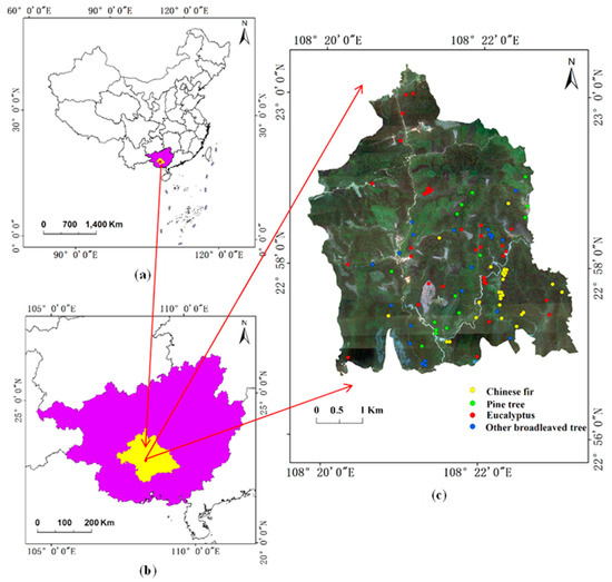
Figure 1.
Location of the study area and the field survey plots ((a) is the location of Guangxi Province. (b) is the location of Nanning City. (c) is the distribution of each species sample plot, the base map is hyperspectral image of the study area).
2.1.2. Field Data
In January 2018, a field survey was conducted in Gaofeng forest farm, Nanning, Guangxi province, and the measured sample plot data were collected. According to the terrain and stand characteristics of the study area, sample plots of different sizes were set up. A total of 98 plots are arranged in the study area, including 27 Chinese fir plots, 15 pine tree plots, 35 eucalyptus plots and 21 other broadleaved tree plots. Other broadleaved trees mainly include Dygoxyllum, Lllicium Linn, Magnolia Denudata, Magnoliaceae Glanca Blume and Erythrophleum Fordii Oliv. The diameter at breast height (DBH) of each tree with DBH greater than 5 cm was measured using DBH ruler, the height of each tree was measured with laser altimeter, the coordinates of each tree were measured with total station, and the coordinates of the center and four corners of the sample plots were measured with RTK. The basic information of the sample plots is shown in Table 1.

Table 1.
Sample plots information.
The AGB of each tree species is calculated using the allometric growth equation of AGB by the measured DBH and tree height. For tree species with more than 20 samples, the number of verification samples is set to a number greater than 10, and the rest are training samples. The tree species with less than 20 samples are modeled and verified by the leave-one method.
2.1.3. Remote Sensing Data
The remote sensing data were obtained by the institute of resource information, Chinese Academy of Forestry Sciences in February 2018 using the Yun-12 fixed wing UAV equipped with RIEGLLMS-Q680i laser scanning system (Horn, Austria) and AISA Eagle II sensor (Oulu, Finland) in sunny weather. The point density of airborne LiDAR point cloud data is 3.35 points/m2, and the data format is .las. The hyperspectral data contains 125 bands, and the data format is .dat. The parameters of laser scanning system are shown in Gao Linghan et al. [33], and the detailed parameters of hyperspectral sensor are shown in Table 2.
Table 2.
The main spatial parameters of hyperspectral system.
2.1.4. Data Preprocessing
The main preprocessing includes radiation calibration, atmosphere correction and terrain radiation correction [34]. Conversion formula was used to complete the radiometric calibration, so as to convert the DN value of the initial image into the radiance value. The fast atmospheric correction method was used to correct the hyperspectral image data, so as to eliminate the influence of atmosphere on the reflection of ground objects [35]. SCS + C correction model is used for terrain correction to eliminate the influence of surface roughness on ground reflectance or brightness [36].
The preprocessing of LiDAR point cloud data is mainly to realize elevation normalization [37]. Firstly, the threshold method is used to remove the noise points generated in the scanning process and retain the important point cloud data in the study area [38,39]. According to the measured forest height, crown width and terrain elevation, the forest threshold range is 0.3~50 m and the search radius is 3 m [40,41]. Secondly, the irregular triangulation filtering TIN algorithm was used to classify the point cloud data and distinguish the ground points and non-ground points [42]. Finally, the ground points were interpolated using TIN interpolation algorithm to generate digital elevation model (DEM) [43], and the non-ground points are interpolated using Kriging interpolation algorithm to generate digital surface model (DSM). The difference operation was performed between DSM and DEM to obtain the canopy height model (CHM). The point cloud data after elevation normalization are shown in Figure 2.
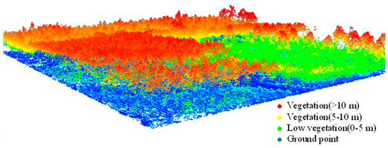
Figure 2.
Elevation normalized point cloud of the study area.
2.2. Methods
2.2.1. Feature Variables Extraction from Hyperspectral Imagery
Hyperspectral imagery has higher spatial resolution and spectral resolution contains richer spectral information and spatial structure information and can obtain more features related to forest AGB. Firstly, the spectral reflectance features, first derivative and second derivative features of 125 bands of hyperspectral data were extracted, respectively (Table 3). Secondly, based on the previous literature [44,45,46], several typical vegetation indices characterizing vegetation coverage and biomass were extracted (Table 4), which included the indices related to atmospheric impedance and topographic characteristics and chlorophyll content and indices representing the characteristics of vegetation leaves. As such, 8 s-order texture features from band 19 (482 nm), band 34 (550 nm) and band 55 (645 nm) were extracted separately based on the GLCM method (Table 5) [47]. These three bands correspond to blue, green and red bands, respectively, with high definition, less interference and obvious ground feature information. In this way, a total of 24 object-based texture features was obtained. Finally, in order to extract more spatial information related to forest structure, wavelet transform [48] and mathematical morphology [49] were used to extract spatial texture features, transformed spectral features and edge features (Table 6).
Table 3.
List of the spectral features for hyperspectral data.
Table 4.
List of the vegetation indices for hyperspectral data.
Table 5.
List of the second-order texture indices calculated by GLCM for hyperspectral data.
Table 6.
List of the spatial texture and transform features for hyperspectral data.
2.2.2. Feature Variables Extraction from LiDAR
According to the data structure features of point cloud data and comprehensively considering the ecological and spatial structure indicators, the feature parameters of point cloud data were extracted from forest canopy information (including canopy density and leaf area index), point cloud structure information (including height percentile, height maximum and minimum), point cloud density information (including point cloud density parameters at different height levels of point cloud) and terrain information (including slope and aspect). For meaning and abbreviation of each feature variable of point cloud data see Gao Linghan et al. [33]. The important features of point cloud data include height percentile and cumulative height percentile. The height percentile refers to the height of X% points in a unit grid. The cumulative height percentile is the height sum of X% points in a unit grid.
2.2.3. Feature Variables of Three-Level Screening and Modeling
In this study, there are many hyperspectral feature parameters and few sample plots. Putting all features into the model will lead to data redundancy, supersaturation of modeling variables and low model accuracy. The following two-level screening scheme was designed for hyperspectral features: First, the extracted feature sets of 11 categories, such as spectral reflectance features, first derivative features, second derivative features, vegetation indices, GLCM texture features, spectral feature of wavelet transform, horizontal texture of wavelet transform, vertical texture of wavelet transform, diagonal texture of wavelet transform, approximate texture of wavelet transform and edge texture, are successively screened for each tree species according to RF method, and modeled separately by multiple stepwise regression method (MSR) [50]. Compare the model accuracy, eliminate the feature sets with model accuracy less than 0.5, and use the remaining feature sets for subsequent screening and modeling. Then, according to the first screening results, RF screening [51] is carried out again to select the corresponding top ranking features of each tree species. Finally, the optimal model of each tree species based on hyperspectral data is obtained by using the MSR method again. According to the number of training samples and the principle of moderate proportion, the proportion of training samples and independent variables is set as 4:1.
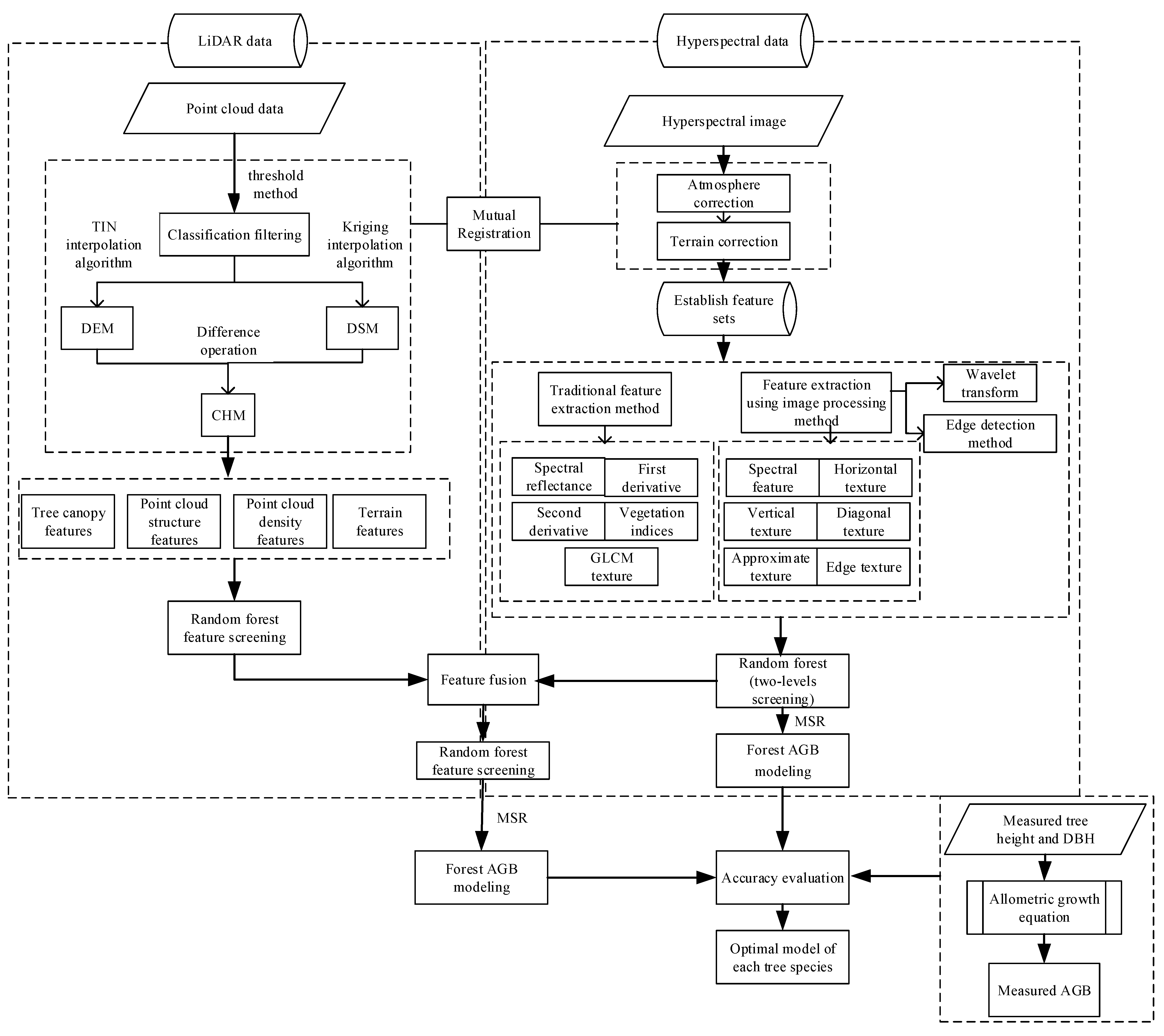
RF method was used to screen the best feature variables derived from airborne LiDAR point cloud data for each tree species. The screening results are shown in Gao Linghan et al. [33]. Then the optimal variables of each tree species screened by airborne hyperspectral and LiDAR data were fused, and the optimal variables of each tree species were screened again by RF method to realize the optimal feature fusion of the two data sources and obtain the final feature variable set. The AGB model of each tree species was established by MSR method to realize the AGB modeling of each tree species based on the feature fusion of multi-source data. The three-level screening and modeling process is shown in Figure 3.
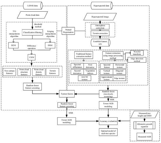
Figure 3.
Three-level screening and modeling process.
The RF method is a popular feature-selection method, which can realize data reduction and optimization. The decline in target prediction accuracy after removing variables is indicated by %IncMSE, which is the growth of root mean square error rate. When the value is larger, the contribution of the variable is greater. Further, %IncMSE formula is shown in Gao Linghan et al. [33]. MSR method considers the variance contribution value of all variables when introducing variables and sorts them into a regression equation according to their importance. The final equation does not contain unnecessary independent variables. The coefficient of determination R2, the root mean square error (RMSE) and mean absolute error (MAE) were used to compare the accuracy. The formula is as follows:
where: R2 is the coefficient of determination, Xobs, i is the measured value, Xmodel, i is the estimated value, and mean is the average value.
where: RMSE is the root mean square error, MAE is the mean absolute error, N is the number of samples.
3. Results
3.1. Hyperspectral Features Selection
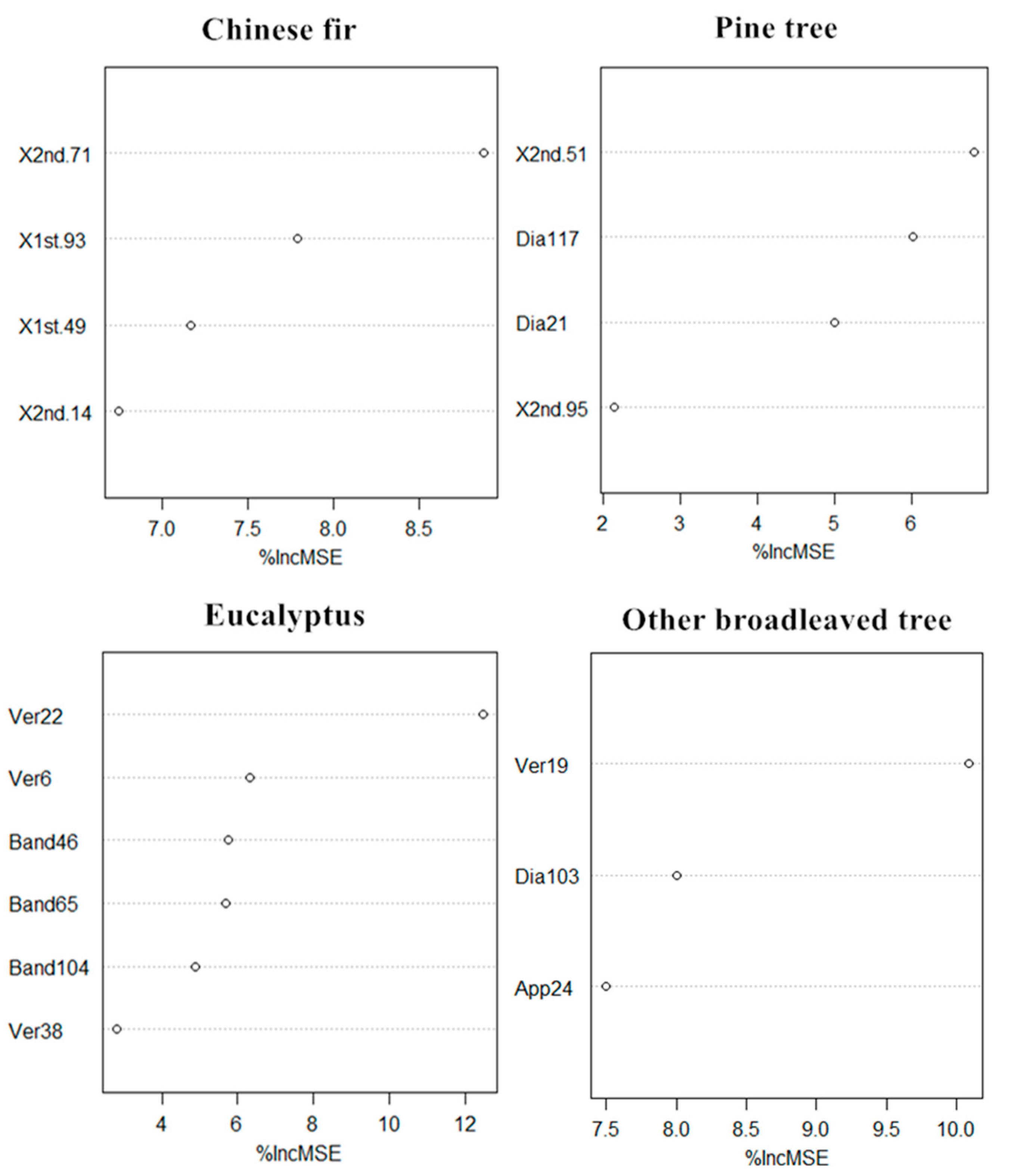
The feature-screening results based on airborne LiDAR data are shown in Gao Linghan et al. [33]. The screening of hyperspectral features eliminates redundant feature parameters and obtains several feature parameters, with the highest correlation between 11 feature sets and AGB of each tree species using the RF method. Four, four, six and three feature parameters were selected for Chinese fir, pine tree, eucalyptus and other broadleaved trees, respectively. The screening results are shown in Figure 4.
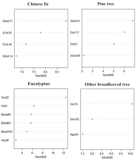
Figure 4.
The feature importance ranking map after two-level screening of hyperspectral features.
It can be seen from Figure 4 that the AGB of Chinese fir has a strong correlation with the derivative features. The AGB of pine trees has a good correlation with the second derivative and the diagonal texture features of wavelet transform, and the texture features of GLCM are removed. The AGB of eucalyptus has a strong correlation with the spectral reflectance features and the vertical texture features of wavelet transform. The AGB of other broadleaved trees has a good correlation with the three texture features of wavelet transform. From the above results, it can be concluded that there is a good correlation between the texture features extracted by wavelet transform and forest AGB, which can be used as an important modeling variable for forest AGB estimation.
3.2. AGB Modeling Using Screened Hyperspectral Features
Based on the features of hyperspectral data screening, the AGB model was constructed by using the multiple stepwise regression method, and its accuracy is shown in Table 7.
Table 7.
Accuracy of AGB model based on hyperspectral data.
It can be seen from Table 7 that the training accuracy of the four tree species is more than 0.75, but the verification accuracy is very different. The training accuracy of pine trees is the best, with accuracy of 0.84, and the verification accuracy is also about 0.8. The training accuracy of Chinese fir is the second. Although the training accuracy of eucalyptus and other broadleaved trees is high, the verification accuracy is very low, indicating that the effect of the model for these two tree species is not ideal, especially the training accuracy and verification accuracy of eucalyptus, as these are all very low. The reason for the deviation between training accuracy and verification accuracy may be that the selected modeling and verification sample plots are uneven, and many attempts can be made in subsequent research. The estimation accuracy of coniferous tree AGB based on hyperspectral data is good, while that of broadleaved tree AGB is low. From the selection of independent variables, it can be seen that coniferous tree AGB is mostly highly correlated with spectral features, broadleaved tree AGB is mostly highly correlated with texture features. Texture features are features after image transformation, and there will be some deviation in calculation, which also makes the estimation results of coniferous tree and broadleaved tree AGB different.
3.3. Feature Screening of LiDAR and Hyperspectral
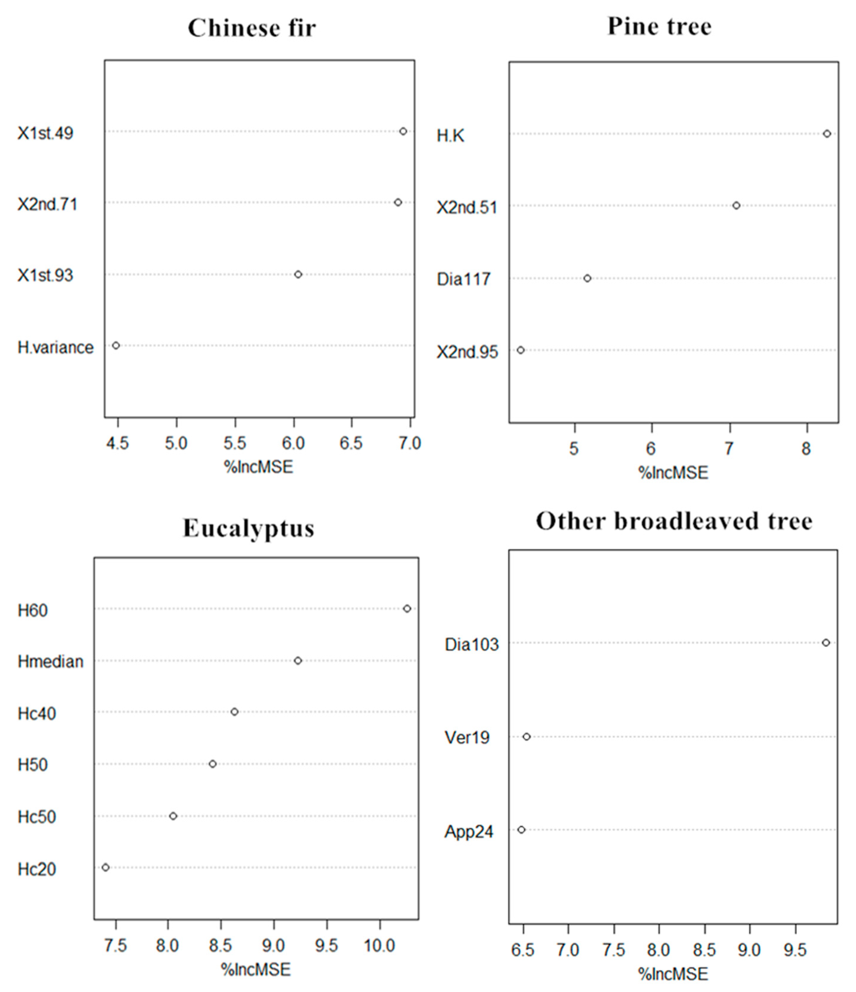
Firstly, the optimal variables extracted from airborne LiDAR data are shown in Gao Linghan et al. [33]. These are basically the point cloud structure features. These features are fused with the optimal features extracted from hyperspectral data for subsequent feature screening. Then, the RF method was used for the three-level screening of features. The ranking results of the importance features of each tree species are shown in Figure 5.
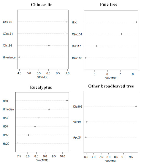
Figure 5.
The feature importance ranking map after three-level screening of fused features.
As can be seen from Figure 5, the feature variables with high importance of Chinese fir and pine trees include features from two data sources, mainly height, spectral and texture features of wavelet transform. The important features of eucalyptus are only correlated with height metrics derived from LiDAR data, and the importance features of other broadleaved trees are texture features of wavelet transform based on hyperspectral data. In terms of tree species structure, eucalyptus belongs to tall trees, with straight and complete trunks and fewer branches. Branches are mostly concentrated in the tree canopy, and the biomass is concentrated in the trunk. Therefore, the biomass is mostly related to the height features. Other broadleaved trees mainly include Castanopsis hystrix Miq., Magnolia denudata Desr., Illicium verum Hook.f., Erythrophleum fordii Oliv. and Magnoliaceae glanca Blume. There is little difference in the height of these tree species, but different tree species have different canopy structure, branch size and leaf shape. Therefore, the forest biomass is mostly related to some shape and texture features. Through the above screening, it can be seen that the AGB of different tree species has the strongest correlation with different features and different data sources.
3.4. AGB Modeling Using Features Fusion
According to the optimal features selected by the three-level screening strategy for each tree species, the AGB models of the four dominant tree species (group) were constructed. The AGB model of other broadleaved trees was constructed based on the features of hyperspectral data (Table 7). The model of eucalyptus was constructed based on the features from airborne LiDAR point cloud data, and the models of Chinese fir and pine tree were constructed based on the fused features of two data sources. The models and accuracy are shown in Table 8.
Table 8.
Modeling accuracy of feature fusion.
It can be seen from Table 8 that the training accuracy of Chinese fir and pine trees is 0.78 and 0.95, respectively, the verification accuracy is 0.44 and 0.91, respectively, and the RMSE is 11.02 and 12.94 t/hm2, respectively. For the pine tree, compared with the modeling results from hyperspectral data, the training accuracy (0.84 based on hyperspectral data) and verification accuracy (0.79 based on hyperspectral data) of the fusion-based model has been greatly improved to 0.95 and 0.91, respectively. For Chinese fir, the training accuracy is slightly lower than that of hyperspectral feature-based modeling (R2 is 0.89), but the verification accuracy (0.38 based on hyperspectral data) is improved to 0.44. The training accuracy of eucalyptus AGB model is 0.72 and the verification accuracy is 0.71. Compared with the modeling results based on hyperspectral data, the verification accuracy of eucalyptus is greatly improved and the training accuracy is reduced by 0.06. After three-level feature screening of other broadleaved trees, the optimal features obtained are the same as those extracted from hyperspectral data. Therefore, the final AGB model results are the same. In summary, AGB models of different tree species based on active and passive data greatly improved the accuracy of Chinese fir, pine tree and eucalyptus, and the AGB of other broadleaved trees has the highest correlation with hyperspectral features.
3.5. Forest Above-Ground Biomass Mapping of the Forest Farm
According to the class II survey data of forest resources in Guangxi Province, the distribution area of each tree species within the forest farm is extracted and the corresponding feature variables in each stand area are extracted. The AGB value of each tree species within the forest farm is estimated by using the optimal model of each tree species based on LiDAR data, based on hyperspectral data and based on fused features. The AGB thematic maps of different tree species in the study area based on the optimal AGB model of different data sources are shown in Figure 6.

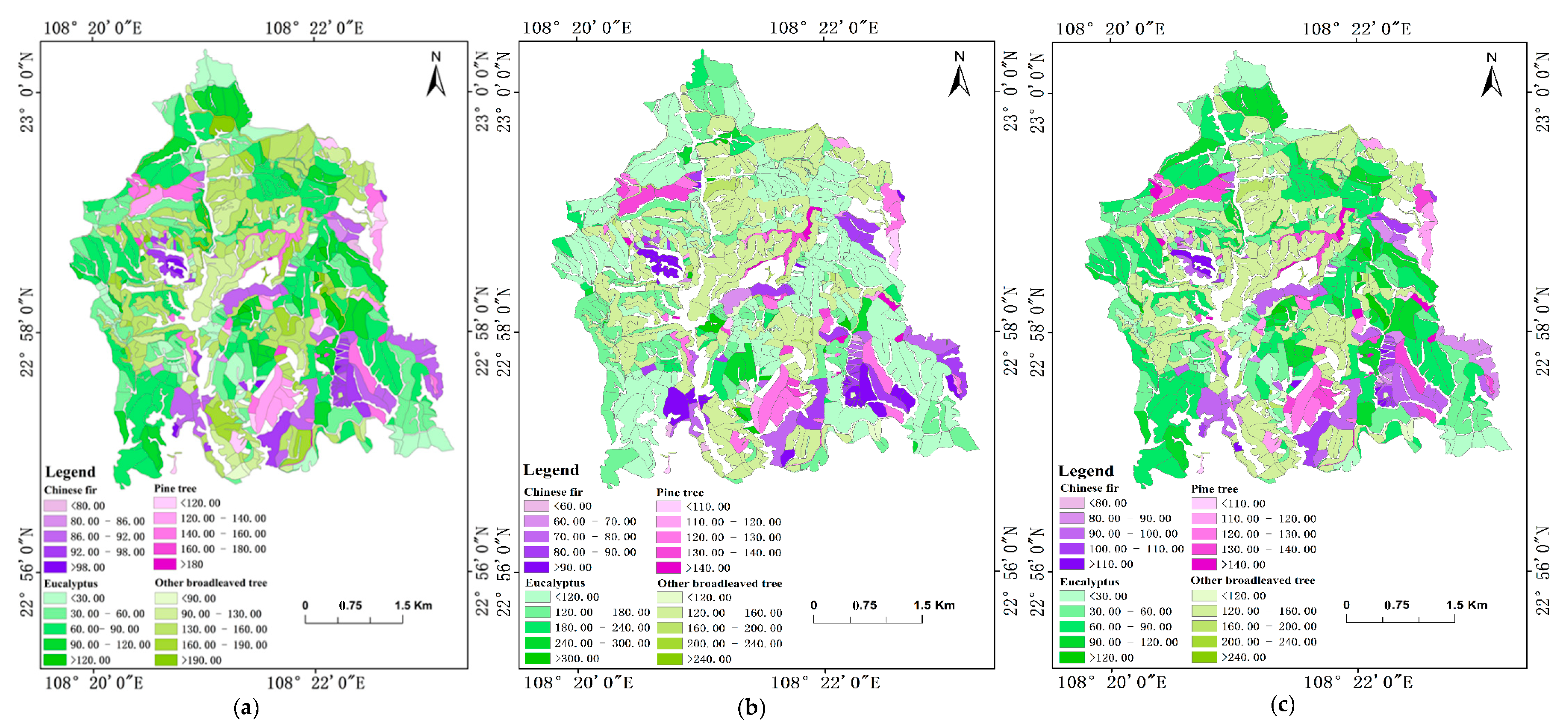
Figure 6.
Distribution of forest AGB in the study area based on different data sources ((a) is the AGB map of each tree species based on airborne LiDAR data. (b) is the AGB map of each tree species based on airborne hyperspectral data. (c) is the AGB map of each tree species based on feature fusion.).
It can be seen from Figure 6 that the spatial distribution law of biomass of each tree species obtained by the three methods is the same. Chinese fir is mainly distributed in the south and central parts of the study area. Pine trees are distributed in a small range, mainly in the northwest and southeast of the study area. Eucalyptuses are mainly distributed in the east and west of the study area; there is a small distribution in the central and north region. Other broadleaved trees are evenly distributed in the central part and around the study area.
Comparing Figure 6b,c, the AGB of Chinese fir in b is mainly concentrated between approximately 70 and 100 t/hm2, and the AGB of Chinese fir in c is mainly concentrated between approximately 75 and 120 t/hm2. The AGB value of Chinese fir estimated based on airborne hyperspectral data is low, and the minimum AGB value of Chinese fir in b is 11.5 t/hm2 and that in c is 77.5 t/hm2. Compared with the measured AGB of Chinese fir, the smallest measured AGB of Chinese fir is 59.2 t/hm2, and most of the Chinese firs in the forest farm are middle aged and mature forests. Therefore, the minimum value of Chinese fir AGB estimation after feature fusion is more accurate.
The AGB of pine trees in b is mainly concentrated between approximately 120 and 130 t/hm2, and in c is mainly concentrated between approximately 120 and 140 t/hm2. The maximum and minimum values in b are 160 t/hm2 and 95 t/hm2, respectively, and the maximum and minimum values in c are 170 t/hm2 and 91 t/hm2, respectively. It can be seen that the biomass estimation value of the area with high AGB is too small based on hyperspectral data.
The maximum AGB of eucalyptus in b is more than 300 t/hm2, and that in c is more than 120 t/hm2. By analyzing the AGB of eucalyptus in small class areas of b and c, respectively, it is found that the maximum AGB of eucalyptus in c is 150 t/hm2, that in b is 700 t/hm2. Compared with the measured AGB of eucalyptus, the measured maximum AGB of eucalyptus is 338.8 t/hm2. It can be concluded that the AGB of eucalyptus in b has a serious oversaturation problem. It shows that the AGB of eucalyptus has little correlation with the features extracted based on hyperspectral data, such as spectral feature and texture feature. The height feature is the key feature to determine the AGB of eucalyptus.
The AGB models of other broadleaved trees in b and c are constructed based on airborne hyperspectral data, and the results are consistent. The AGB of other broadleaved trees in a is calculated based on the optimal model of LiDAR data. The AGB values of other broadleaved trees are mostly between approximately 130 and 190 t/hm2, and the AGB values of other broadleaved trees in c are mostly between approximately 120 and 160 t/hm2, indicating that the AGB values of other broadleaved trees calculated based on LiDAR data are generally greater than those calculated based on feature fusion.
In summary, feature fusion based on different data sources can avoid the problem of data value oversaturation. The estimation results of Chinese firs and pine trees based on feature fusion are better, the results of eucalyptuses based on LiDAR data are the best, and the estimation results of other broadleaved trees based on hyperspectral data are the best.
4. Discussion
4.1. Significance of Multi-Level Feature Screening
In this study, airborne LiDAR point cloud data and hyperspectral data were used to analyze the optimal feature variables of AGB modeling and the AGB estimation models of different tree species were established in a complex plantation in China. The three-level feature screening strategy was adopted in the feature screening of multi-source data. The airborne LiDAR features and hyperspectral features were screened, respectively, and then the fused features of the two data sources were screened. Finally, the selection of the optimal features was completed. At the same time, in the feature screening of hyperspectral data, two-level screening are also carried out. First, the feature screening was carried out based on different feature sets, and then, the final optimal hyperspectral features were screened based on the optimal feature sets. This hierarchical screening strategy can effectively avoid the problem of feature redundancy and effectively reduce irrelevant features in the case of few measured samples.
4.2. Selection of Optimal Feature Variables of Different Tree Species
The optimal feature variables of different tree species are related to the tree structures. Compared with most previous studies, the estimation accuracy of AGB is mostly related to vegetation index and point cloud height features [20,25]. In this study, the best features of Chinese firs and pine trees include spectral derivative features, point cloud height features and wavelet transform texture features. The best feature of eucalyptus is the height feature of point cloud, and the best feature of other broadleaved trees is the texture feature of wavelet transform. This shows that the optimal features of different tree species are different due to the specific vertical and canopy structure, and the texture features extracted by wavelet transform can be used for forest AGB modeling. In the subsequent forest AGB research, the corresponding remote sensing data can be selected according to different tree species to extract relevant feature variables.
4.3. Importance of Tree Species AGB Modeling
It is necessary to distinguish tree species to estimate the AGB models. Based on the optimal features of different data sources, using the MSR method to construct the AGB model by tree species can effectively avoid the problem that the previous AGB model is not targeted. More accurate mapping results can be obtained for forest AGB estimation and large-scale regional mapping with complex tree species composition and structural heterogeneity. At the same time, the canopy structure and tree shape of different tree species are different, and the carbon sequestration capacity is also different [21]. Distinguishing tree species to construct AGB models can improve the estimation accuracy of each tree species and also provide a more accurate reference basis for carbon reserve estimation.
4.4. Existing Problems and Future Research Directions
This study only studies the forest AGB model of Gaofeng forest farm in Nanning, Guangxi. There is no comparative analysis on whether the same tree species in other areas can use the model of this study. It can be extended in the follow-up study. At the same time, this study uses the method of feature fusion to combine the two data sources. Later, we can carry out further research on different data-source fusion methods.
5. Conclusions
This study explored the impact of a single remote sensing data source and active and passive remote sensing data fusion on the estimation accuracy of AGB of different tree species. In data feature extraction, according to the characteristics of different data sources, the feature set was constructed from tree canopy features, point cloud structure features, point cloud density features, terrain features, spectral reflectance, spectral derivative, GLCM texture, wavelet transform features and edge detection features. After three-level feature screening and modeling, the optimal models of AGB of different tree species were obtained. The results are as follows:
- (a)
- Based on airborne hyperspectral data, the feature set was constructed by using multiple band combinations, wavelet transform and edge detection methods. Through two-level screening and modeling, it can be concluded that vegetation index and texture features based on GLCM have no obvious effect on improving the accuracy of the AGB model. Spectral features and texture features of wavelet transform play a decisive role in the construction of the AGB model. The AGB accuracy of the optimal models of the four tree species based on the optimal features of hyperspectral data was higher than 0.78, but the verification accuracy was very different. The verification accuracy of eucalyptus was only 0.03, which has the problem of over fitting. In conclusion, modeling using only hyperspectral data will have an impact on the estimation results of eucalyptus AGB. This is because for tall tree species, height features are also an important factor affecting the estimation accuracy of AGB.
- (b)
- AGB models of different tree species were constructed based on multi-source feature fusion. From the results of feature screening, it can be concluded that the optimal features of Chinese firs and pine trees included the features of two data sources. Eucalyptus AGB had the best correlation with LiDAR point cloud data. The top features of other broadleaved trees were the features extracted from hyperspectral data. The training accuracy of the AGB model for each tree species was more than 0.72, and the verification accuracy was quite different. However, after feature fusion, the verification accuracy of Chinese firs and pine trees was improved. The results showed that AGB estimation and mapping in areas with complex tree species composition and high structural heterogeneity must be modeled by tree species. For coniferous trees, the AGB model constructed by combining airborne LiDAR height features and hyperspectral texture features had higher accuracy. The optimal features of the broadleaved tree AGB model will have different choices according to different tree species. For tall broadleaved trees, the AGB model based on airborne LiDAR height features had higher accuracy. Meanwhile, the AGB model for pure forests, such as Chinese firs, pine trees and eucalyptuses, can also be based on the above conclusions.
Author Contributions
L.G., Investigation, Methodology, Software, Validation, Visualization, Writing—original draft; G.C., Validation, Visualization; X.Z., Funding acquisition, Project administration, Resources. All authors have read and agreed to the published version of the manuscript.
Funding
This research was funded by the NSFC (32171779) and National Ministry of Science and Technology [grant number 2017YFD0600900].
Acknowledgments
We would like to thank the Gaofeng Forest Farm in Nanning City, Guangxi Province, for their aid during the field survey. We would also like to thank Erxue Chen and Lei Zhao from the Institute of Forest Resource Information Techniques CAF and Yueting Wang, Kaili Cao, Zhengqi Guo and Xuemei Zhou from Beijing Forestry University for their help in the field work.
Conflicts of Interest
The authors declare that they have no known competing financial interests or personal relationships that could have appeared to influence the work reported in this paper.
References
- Fassnacht, F.; Hartig, F.; Latifi, H.; Berger, C.; Hernández, J.; Corvalán, P.; Koch, B. Importance of sample size, data type and prediction method for remote sensing-based estimations of aboveground forest biomass. Remote Sens. Environ. 2014, 154, 102–114. [Google Scholar] [CrossRef]
- Castillo, J.A.A.; Apan, A.A.; Maraseni, T.N.; Salmo, S.G., III. Estimation and mapping of above-ground biomass of mangrove forests and their replacement land uses in the Philippines using Sentinel imagery. ISPRS J. Photogramm. Remote Sens. 2017, 134, 70–85. [Google Scholar] [CrossRef]
- Ratle, F.; Camps-Valls, G.; Weston, J. Semisupervised neural networks for efficient hyperspectral image classification. IEEE Trans. Geosci. Remote Sens. 2010, 48, 2271–2282. [Google Scholar] [CrossRef]
- García, M.; Riaño, D.; Chuvieco, E.; Danson, F.M. Estimating biomass carbon stocks for a Mediterranean forest in central Spain using LiDAR height and intensity data. Remote Sens. Environ. 2010, 114, 816–830. [Google Scholar] [CrossRef]
- Propastin, P. Modifying geographically weighted regression for estimating aboveground biomass in tropical rainforests by multispectral remote sensing data. Int. J. Appl. Earth Obs. Geoinf. 2012, 18, 82–90. [Google Scholar] [CrossRef]
- Kankare, V.; Vastaranta, M.; Holopainen, M.; Räty, M.; Yu, X.; Hyyppä, J.; Hyyppä, H.; Alho, P.; Viitala, R. Retrieval of forest aboveground biomass and stem volume with airborne scanning LiDAR. Remote Sens. 2013, 5, 2257–2274. [Google Scholar] [CrossRef] [Green Version]
- Cutler, M.; Boyd, D.; Foody, G.; Vetrivel, A. Estimating tropical forest biomass with a combination of SAR image texture and Landsat TM data: An assessment of predictions between regions. ISPRS J. Photogramm. Remote Sens. 2012, 70, 66–77. [Google Scholar] [CrossRef] [Green Version]
- Estornell, J.; Ruiz, L.; Velázquez-Martí, B.; Fernández-Sarría, A. Estimation of shrub biomass by airborne LiDAR data in small forest stands. For. Ecol. Manag. 2011, 262, 1697–1703. [Google Scholar] [CrossRef] [Green Version]
- Güneralp, İ.; Filippi, A.M.; Randall, J. Estimation of floodplain aboveground biomass using multispectral remote sensing and nonparametric modeling. Int. J. Appl. Earth Obs. Geoinf. 2014, 33, 119–126. [Google Scholar] [CrossRef]
- Wallis, C.I.; Homeier, J.; Peña, J.; Brandl, R.; Farwig, N.; Bendix, J. Modeling tropical montane forest biomass, productivity and canopy traits with multispectral remote sensing data. Remote Sens. Environ. 2019, 225, 77–92. [Google Scholar] [CrossRef]
- Liu, Y.; Gong, W.; Xing, Y.; Hu, X.; Gong, J. Estimation of the forest stand mean height and aboveground biomass in Northeast China using SAR Sentinel-1B, multispectral Sentinel-2A, and DEM imagery. ISPRS J. Photogramm. Remote Sens. 2019, 151, 277–289. [Google Scholar] [CrossRef]
- Wittke, S.; Yu, X.; Karjalainen, M.; Hyyppä, J.; Puttonen, E. Comparison of two-dimensional multitemporal Sentinel-2 data with three-dimensional remote sensing data sources for forest inventory parameter estimation over a boreal forest. Int. J. Appl. Earth Obs. Geoinf. 2019, 76, 167–178. [Google Scholar] [CrossRef]
- Zhong, Y.; Zhang, L. An adaptive artificial immune network for supervised classification of multi-/hyperspectral remote sensing imagery. IEEE Trans. Geosci. Remote Sens. 2011, 50, 894–909. [Google Scholar] [CrossRef]
- Brantley, S.T.; Zinnert, J.C.; Young, D.R. Application of hyperspectral vegetation indices to detect variations in high leaf area index temperate shrub thicket canopies. Remote Sens. Environ. 2011, 115, 514–523. [Google Scholar] [CrossRef] [Green Version]
- Van der Meer, F.D.; Van der Werff, H.M.; Van Ruitenbeek, F.J.; Hecker, C.A.; Bakker, W.H.; Noomen, M.F.; Van Der Meijde, M.; Carranza, E.J.M.; De Smeth, J.B.; Woldai, T. Multi-and hyperspectral geologic remote sensing: A review. Int. J. Appl. Earth Obs. Geoinf. 2012, 14, 112–128. [Google Scholar] [CrossRef]
- Halme, E.; Pellikka, P.; Mõttus, M. Utility of hyperspectral compared to multispectral remote sensing data in estimating forest biomass and structure variables in Finnish boreal forest. Int. J. Appl. Earth Obs. Geoinf. 2019, 83, 101942. [Google Scholar] [CrossRef]
- Cooper, S.; Okujeni, A.; Pflugmacher, D.; van der Linden, S.; Hostert, P. Combining simulated hyperspectral EnMAP and Landsat time series for forest aboveground biomass mapping. Int. J. Appl. Earth Obs. Geoinf. 2021, 98, 102307. [Google Scholar] [CrossRef]
- Koch, B. Status and future of laser scanning, synthetic aperture radar and hyperspectral remote sensing data for forest biomass assessment. ISPRS J. Photogramm. Remote Sens. 2010, 65, 581–590. [Google Scholar] [CrossRef]
- Silva, C.A.; Klauberg, C.; Hudak, A.T.; Vierling, L.A.; Liesenberg, V.; Carvalho, S.P.E.; Rodriguez, L.C. A principal component approach for predicting the stem volume in Eucalyptus plantations in Brazil using airborne LiDAR data. For. Int. J. For. Res. 2016, 89, 422–433. [Google Scholar] [CrossRef]
- Fassnacht, F.E.; Latifi, H.; Hartig, F. Using synthetic data to evaluate the benefits of large field plots for forest biomass estimation with LiDAR. Remote Sens. Environ. 2018, 213, 115–128. [Google Scholar] [CrossRef]
- Cao, L.; Coops, N.C.; Sun, Y.; Ruan, H.; Wang, G.; Dai, J.; She, G. Estimating canopy structure and biomass in bamboo forests using airborne LiDAR data. ISPRS J. Photogramm. Remote Sens. 2019, 148, 114–129. [Google Scholar] [CrossRef]
- Luo, S.; Wang, C.; Xi, X.; Pan, F.; Peng, D.; Zou, J.; Nie, S.; Qin, H. Fusion of airborne LiDAR data and hyperspectral imagery for aboveground and belowground forest biomass estimation. Ecol. Indic. 2017, 73, 378–387. [Google Scholar] [CrossRef]
- Wu, Z.; Dye, D.; Vogel, J.; Middleton, B. Estimating forest and woodland aboveground biomass using active and passive remote sensing. Photogramm. Eng. Remote Sens. 2016, 82, 271–281. [Google Scholar] [CrossRef]
- García, M.; Saatchi, S.; Ustin, S.; Balzter, H. Modelling forest canopy height by integrating airborne LiDAR samples with satellite Radar and multispectral imagery. Int. J. Appl. Earth Obs. Geoinf. 2018, 66, 159–173. [Google Scholar] [CrossRef]
- Abutaleb, K.; Newete, S.W.; Mangwanya, S.; Adam, E.; Byrne, M.J. Mapping eucalypts trees using high resolution multispectral images: A study comparing WorldView 2 vs. SPOT 7. Egypt. J. Remote Sens. Space Sci. 2021, 24, 333–342. [Google Scholar] [CrossRef]
- Baccini, A.; Laporte, N.; Goetz, S.; Sun, M.; Dong, H. A first map of tropical Africa’s above-ground biomass derived from satellite imagery. Environ. Res. Lett. 2008, 3, 045011. [Google Scholar] [CrossRef] [Green Version]
- Boudreau, J.; Nelson, R.F.; Margolis, H.A.; Beaudoin, A.; Guindon, L.; Kimes, D.S. Regional aboveground forest biomass using airborne and spaceborne LiDAR in Québec. Remote Sens. Environ. 2008, 112, 3876–3890. [Google Scholar] [CrossRef]
- Chen, G.; Hay, G.J. A support vector regression approach to estimate forest biophysical parameters at the object level using airborne LiDAR transects and quickbird data. Photogramm. Eng. Remote Sens. 2011, 77, 733–741. [Google Scholar] [CrossRef] [Green Version]
- Laurin, G.V.; Chen, Q.; Lindsell, J.A.; Coomes, D.A.; Del Frate, F.; Guerriero, L.; Pirotti, F.; Valentini, R. Aboveground biomass estimation in an African tropical forest with LiDAR and hyperspectral data. ISPRS J. Photogramm. Remote Sens. 2014, 89, 49–58. [Google Scholar] [CrossRef]
- Li, L.; Guo, Q.; Tao, S.; Kelly, M.; Xu, G. LiDAR with multi-temporal MODIS provide a means to upscale predictions of forest biomass. ISPRS J. Photogramm. Remote Sens. 2015, 102, 198–208. [Google Scholar] [CrossRef]
- De Almeida, C.T.; Galvao, L.S.; Ometto, J.P.H.B.; Jacon, A.D.; de Souza Pereira, F.R.; Sato, L.Y.; Lopes, A.P.; de Alencastro Graça, P.M.L.; de Jesus Silva, C.V.; Ferreira-Ferreira, J. Combining LiDAR and hyperspectral data for aboveground biomass modeling in the Brazilian Amazon using different regression algorithms. Remote Sens. Environ. 2019, 232, 111323. [Google Scholar] [CrossRef]
- Wang, D.; Wan, B.; Liu, J.; Su, Y.; Guo, Q.; Qiu, P.; Wu, X. Estimating aboveground biomass of the mangrove forests on northeast Hainan Island in China using an upscaling method from field plots, UAV-LiDAR data and Sentinel-2 imagery. Int. J. Appl. Earth Obs. Geoinf. 2020, 85, 101986. [Google Scholar] [CrossRef]
- Gao, L.; Zhang, X. Aboveground biomass estimation of plantation with complex forest stand structure using multiple features from airborne laser scanning point cloud data. Forests 2021, 12, 1713. [Google Scholar] [CrossRef]
- Guo, B.; Gunn, S.R.; Damper, R.I.; Nelson, J.D. Customizing kernel functions for SVM-based hyperspectral image classification. IEEE Trans. Image Process. 2008, 17, 622–629. [Google Scholar] [CrossRef] [Green Version]
- Fauvel, M.; Tarabalka, Y.; Benediktsson, J.A.; Chanussot, J.; Tilton, J.C. Advances in spectral-spatial classification of hyperspectral images. Proc. IEEE 2012, 101, 652–675. [Google Scholar] [CrossRef] [Green Version]
- Soenen, S.A.; Peddle, D.R.; Coburn, C.A. SCS+ C: A modified sun-canopy-sensor topographic correction in forested terrain. IEEE Trans. Geosci. Remote Sens. 2005, 43, 2148–2159. [Google Scholar] [CrossRef]
- Yang, X. Cover: Use of LIDAR elevation data to construct a high-resolution digital terrain model for an estuarine marsh area. Int. J. Remote Sens. 2005, 26, 5163–5166. [Google Scholar] [CrossRef]
- Zhou, S.; Liu, X.; Wang, C.; Yang, B. Non-iterative denoising algorithm based on a dual threshold for a 3D point cloud. Opt. Lasers Eng. 2020, 126, 105921. [Google Scholar] [CrossRef]
- Gorgens, E.B.; Valbuena, R.; Rodriguez, L.C.E. A method for optimizing height threshold when computing airborne laser scanning metrics. Photogramm. Eng. Remote Sens. 2017, 83, 343–350. [Google Scholar] [CrossRef]
- Zhang, Y.; Lyu, X. A three-dimensional diffusion filtering model establishment and analysis for point cloud intensity noise. J. Comput. Inf. Sci. Eng. 2017, 17, 011010. [Google Scholar] [CrossRef]
- Bayram, E.; Frossard, P.; Vural, E.; Alatan, A. Analysis of airborne LiDAR point clouds with spectral graph filtering. IEEE Geosci. Remote Sens. Lett. 2018, 15, 1284–1288. [Google Scholar] [CrossRef] [Green Version]
- Liu, H.; Wu, C. Developing a scene-based triangulated irregular network (TIN) technique for individual tree crown reconstruction with LiDAR data. Forests 2019, 11, 28. [Google Scholar] [CrossRef] [Green Version]
- Polat, N.; Uysal, M.; Toprak, A.S. An investigation of DEM generation process based on LiDAR data filtering, decimation, and interpolation methods for an urban area. Measurement 2015, 75, 50–56. [Google Scholar] [CrossRef]
- Mutanga, O.; Skidmore, A.K. Narrow band vegetation indices overcome the saturation problem in biomass estimation. Int. J. Remote Sens. 2004, 25, 3999–4014. [Google Scholar] [CrossRef]
- Behmann, J.; Steinrücken, J.; Plümer, L. Detection of early plant stress responses in hyperspectral images. ISPRS J. Photogramm. Remote Sens. 2014, 93, 98–111. [Google Scholar] [CrossRef]
- Tong, X.; Duan, L.; Liu, T.; Singh, V.P. Combined use of in situ hyperspectral vegetation indices for estimating pasture biomass at peak productive period for harvest decision. Precis. Agric. 2019, 20, 477–495. [Google Scholar] [CrossRef]
- Aasen, H.; Burkart, A.; Bolten, A.; Bareth, G. Generating 3D hyperspectral information with lightweight UAV snapshot cameras for vegetation monitoring: From camera calibration to quality assurance. ISPRS J. Photogramm. Remote Sens. 2015, 108, 245–259. [Google Scholar] [CrossRef]
- Rai, H.M.; Chatterjee, K. Hybrid adaptive algorithm based on wavelet transform and independent component analysis for denoising of MRI images. Measurement 2019, 144, 72–82. [Google Scholar] [CrossRef]
- Bi, B.; Zeng, L.; Shen, K.; Jiang, H. An effective edge extraction method using improved local binary pattern for blurry digital radiography images. NDT E Int. 2013, 53, 26–30. [Google Scholar] [CrossRef]
- Chen, W.; Zhao, J.; Cao, C.; Tian, H. Shrub biomass estimation in semi-arid sandland ecosystem based on remote sensing technology. Glob. Ecol. Conserv. 2018, 16, e00479. [Google Scholar] [CrossRef]
- Sun, Q. Research on the driving factors of energy carbon footprint in Liaoning province using random forest algorithm. Appl. Ecol. Environ. Res. 2019, 17, 8381–8394. [Google Scholar] [CrossRef]


Publisher’s Note: MDPI stays neutral with regard to jurisdictional claims in published maps and institutional affiliations. |
© 2022 by the authors. Licensee MDPI, Basel, Switzerland. This article is an open access article distributed under the terms and conditions of the Creative Commons Attribution (CC BY) license (https://creativecommons.org/licenses/by/4.0/).