Abstract
Hyperspectral drill-core scanning adds value to exploration campaigns by providing continuous, high-resolution mineralogical data over the length of entire boreholes. However, multivariate mineralogical data must be transformed into lithological domains such that it is compatible with interpolation techniques and be usable for geomodeling. Manual interpretation of multivariate drill-core data is a challenging, time-consuming and subjective task, and automated or semi-automated approaches are needed. However, naive machine-learning techniques that ignore the distinct spatial structure and multi-scale nature of geological systems tend to produce geologically unreasonable results. Automated geological logging and multi-scale hierarchical domaining of drill-cores has been previously addressed in several studies by means of scalograms from a wavelet transform and tessellation, albeit exploiting only univariate information. The methodology involves the extraction of the local first principal component at a neighborhood of each observation, and the segmentation of the resulting series of scores with a continuous wavelet transform for boundary detection. In this way, the correlation pattern between the variables is incorporated into the segmentation. The scalogram accurately locates the geological boundaries at depth and yields hierarchical geological domains with mineralogical composition characteristics. The performance of this approach is demonstrated on a synthetic as well as a real multivariate dataset. The real dataset consists of mineral abundances derived from drill-core hyperspectral imaging data acquired in Elvira, a shale-hosted volcanogenic massive sulfide deposit located in the Iberian Pyrite Belt, where 7000 m of drill-core were acquired along 80 boreholes. The extracted domains are sensible from a geological point of view and spatially coherent across the boreholes in cross-sections. The results at relevant scales were qualitatively validated by comparing against the lithological log. This method is fast, is appropriate for multivariate geological data along boreholes, and provides a choice of scales for hierarchical geological domains along boreholes with mineralogical composition characteristics that can be modeled in 3D. Our approach provides an automatic way to transform hyperspectral image-derived mineral maps into vertically coherent geological units that are appropriate inputs for 3D geological modeling workflows. Moreover, the method improves the boundary detection and geological domaining by making use of multivariate information.
1. Introduction
Drill-cores are samples of the geological subsurface that are used in the mining industry for deposit characterization. In most cases, the material of drill-cores is visually logged by geologists, which is labor-intensive, and prone to biases and inconsistencies. Hyperspectral imaging (HSI) of drill-cores is a data-driven and thus more objective alternative to visual drill-core logging. It provides fast, high-resolution, spatially continuous, reproducible and non-destructive mapping of minerals over the length of entire boreholes [1,2,3,4,5,6,7]. However, although drill-core HSI is being adopted by geological surveys and the mining industry [8], there are remaining challenges for the technique to become useful for 3D resource geomodeling at the scale of an entire mineral deposit: (i) the automated processing of large quantities of hyperspectral data; (ii) the lack of a clear workflow to derive geologically meaningful domains; (iii) the effect of scale impacts the consistency of classifications between domains extracted from different boreholes; and (iv) the integration and interpolation of domains as categorical results in the 3D modeling. Hyperspectral data can provide mineral or alteration indices that can be used as a proxy in 3D models of mineralization (e.g., Lypaczewski et al., 2020 [7]), but are insufficient input for the detailed modeling of geologically meaningful domains. We recently addressed the challenge arising from automated processing of large quantities of hyperspectral data to produce quantitative mineralogical data at the deposit-scale [9].
This workflow produces a multivariate dataset of downhole mineral abundance from drill-core hyperspectral data. The extraction of lithological domains is possible due to the lithological control on mineral distributions. Therefore, both numerical and categorical results can be integrated in a combined 3D modeling approach. Automatically extracting lithological contacts from mineral abundance data has the advantage of providing consistency across boreholes and overcoming the discrepancies which could be caused by the diverse interpretations of different geologists. To properly obtain geologically meaningful domains that can be integrated into 3D geological modeling, the multivariate dataset of downhole mineral abundance must be segmented into lithological domains. This requires taking into account (i) the multi-scale nature of the geological data and (ii) the fact that some lithological changes are only apparent in the correlation of the variables. The state-of-the-art segmentation method that can be applied to borehole logging data and preserve the multi-scale nature of the data is the continuous wavelet transform (CWT) method. The CWT is a wavelet-based analysis for signal decomposition [10]. This method has been widely applied in the image analysis field for boundary detection [11,12]. The method has also been applied on datasets derived from geophysical and geochemical measurements and has shown good results when applied to univariate datasets [13,14]. Several authors have presented CWT-based methodologies for multivariate datasets aiming at automated geological logging and hierarchical domaining of drill-cores by means of scalograms and tessellation [15,16,17,18] where the boundaries of each variable are extracted individually in a univariate way and then the boundaries are additively combined in a post-processing stage. Some downsides of this approach are that it does not take into account that some lithological changes are only apparent in the correlation of the variables, and it is not a practical solution for datasets with a high number of variables. Recent alternative methods incorporate multivariate analysis within the boundary-detection algorithms using hyperspectral data [18]. Nevertheless, the potential of hyperspectral data is not fully used when the reflectance values of each spectral band are individually implemented as multivariate input data. In our proposed method the raw hyperspectral data cube is not used directly as an input multivariate dataset since the individual reflectance values of each band cannot be directly associated with one specific mineral. Furthermore, reflectance values can vary depending on sensor type, sensor noise, lighting conditions, grain size, etc. [1,19]. In order to obtain mineral information from hyperspectral data, spectrum features should be extracted, the data must be processed and classified. Absorption feature characteristics such as the wavelength position of the deepest absorption, depth of the absorption and symmetry of the absorption feature can be derived from hyperspectral data and used as a proxy for mineral chemistry [20]. In order to produce geologically meaningful results, mineral abundances derived from hyperspectral data processing can be used as input multivariate dataset following [9].
In this paper, we present an open-source toolbox based on the CWT method that provides an automatic procedure to transform HSI-derived mineral abundance logs into multi-scale geological units that can serve as an appropriate input for 3D geological modeling workflows. One of the innovations of our approach is that we incorporate the correlations between multiple variables into the actual segmentation by performing a moving-window principal component analysis along depth, taking full advantage of the multivariate nature of the data. In this way, we improve the detection sensitivity of lithological contacts compared to the state-of-the-art tessellation approaches that are based on boundary extraction of each variable and subsequent combination. This method is fast, appropriate for multivariate geological data along boreholes and provides a choice of scales for hierarchical geological domains along boreholes with mineralogical composition characteristics that can be modeled in 3D. The proposed methodology provides a useful tool to geologists to assist and complement the manual drill-core-logging process. This approach adds tremendous value to core data, allowing a better understanding of geological settings in mineral deposits and providing valuable insights in exploration targeting. In order to allow a large use, we provide the codes as open-source.
2. Methodology
In this section, we describe the methodology to derive multi-scale lithological logs of geological domains from a multivariate dataset. This method is developed for multivariate mineral abundances data derived from the processing of drill-core hyperspectral images. However, it is flexible enough to accept different multivariate datasets as input data such as a collection of geophysical logs or an X-ray fluorescence core scan. To evaluate the accuracy of the method, a synthetic dataset is introduced. A real dataset is used to demonstrate the usefulness of the method.
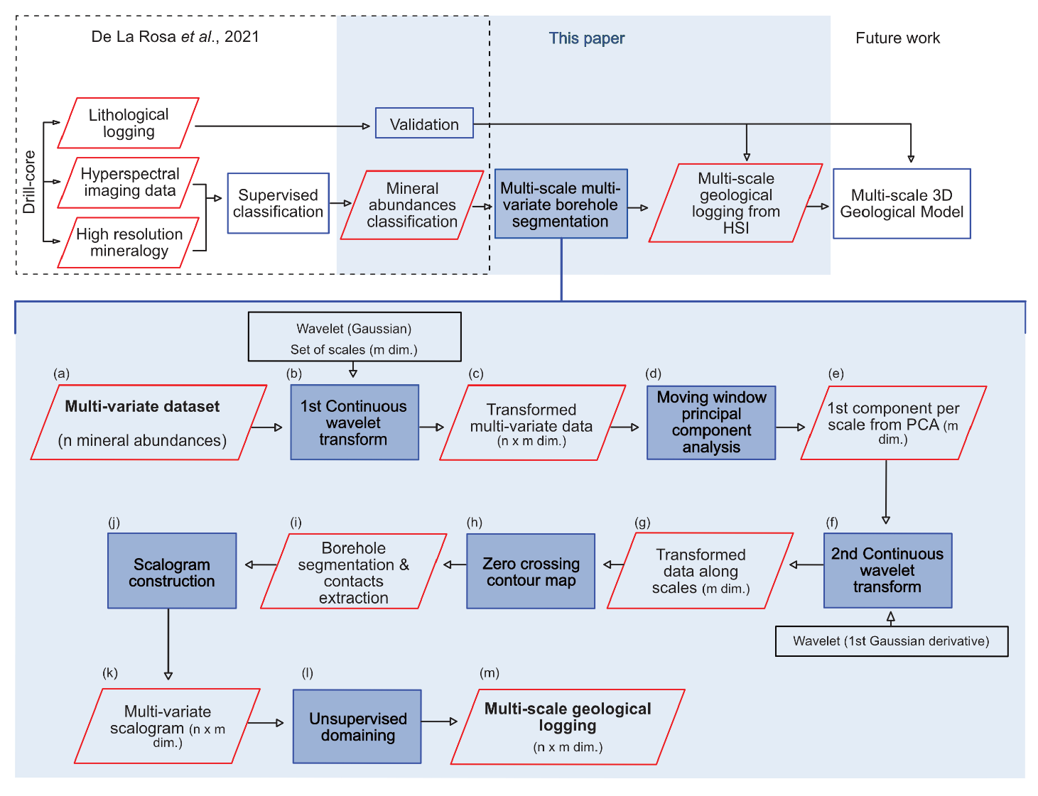
Panels a–m of Figure 1 illustrate step by step the workflow of the proposed methodology from input data to final results. Following subsections explain in detail each step of this workflow. Furthermore, Figure 2 illustrates each step of the workflow with results obtained from the synthetic dataset. The method employs signal decomposition techniques at various scales by means of the wavelet transform and extracts the location of inflection points in the data. By introducing a principal component analysis along moving windows, the algorithm takes full advantage of the multivariate nature of the data. The produced outcome is a scalogram, which is a segmentation of the borehole logs at different scales. Together with the multivariate information, the scalogram is then fed into an unsupervised classification algorithm to obtain domains across boreholes and along each borehole at different scales. The vertical coherence, the lateral continuity and the mineral abundance variability in each domain allows the interpretation of these domains geologically.
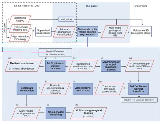
Figure 1.
General workflow for multi-scale, multivariate borehole segmentation from hyperspectral drill-core data [9]. Panels (a,c,e,g,i,k,m) with outer red border represents the input and output data for each step of the method workflow. Panels (b,d,f,h,j,l) represents the main steps for the multi-scale multivariate borehole segmentation method.

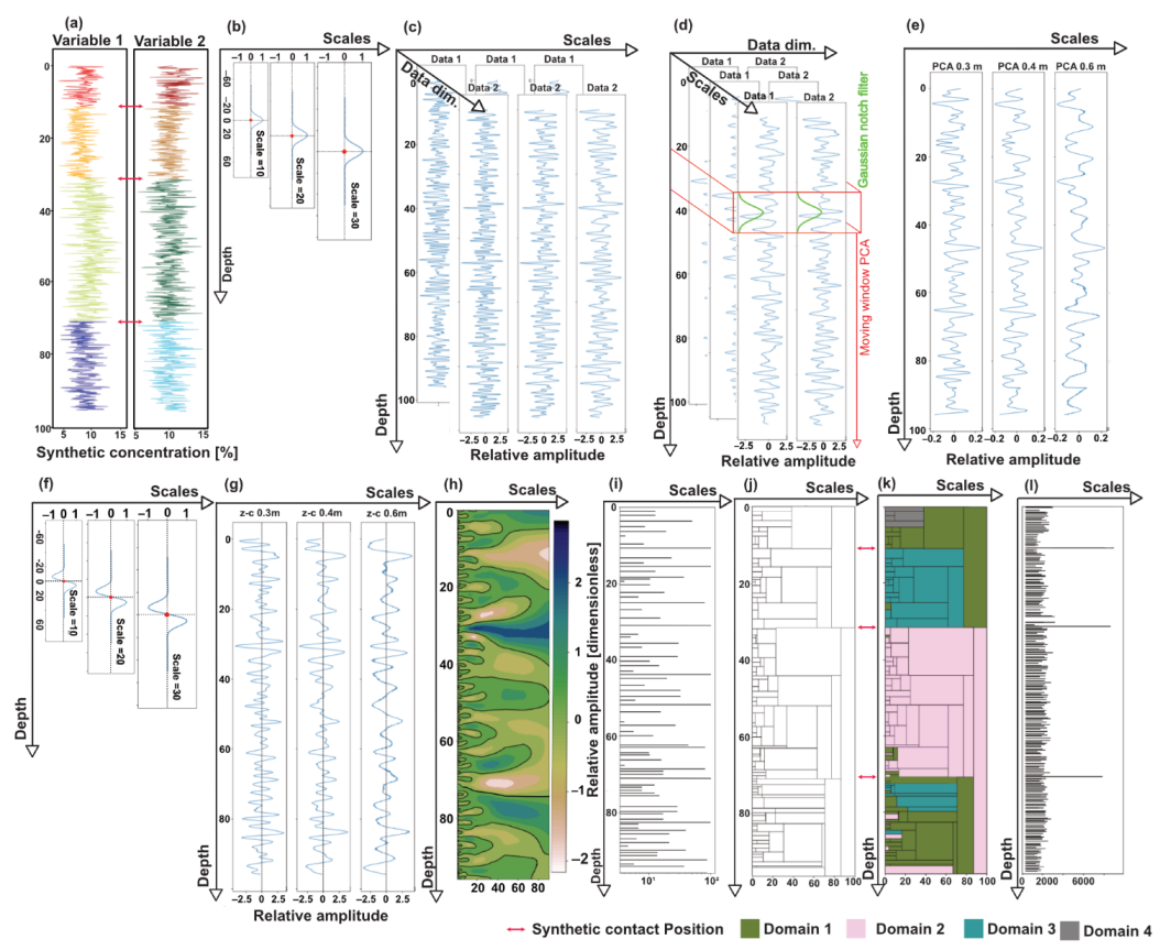
Figure 2.
Illustrated workflow applied on a synthetic example. (a) Raw multivariate data. The colour scheme of the variables in panel (a) is explained in Figure 3. (b) Gaussian functions stretched along the scales, which are used as wavelets for the CWT. (c) multivariate and multi-scale output after applying the CWT with Gaussian wavelet. (d) Illustration of moving-window PCA and Gaussian notch filter. (e) First PCA component for each scale. (f) First derivative of Gaussian functions stretched along the scales, which are used as wavelets for the second CWT. (g) Zero-crossing resulting values along scales. (h) Contourmap of zero-crossing values along scales. (i) Geological domains extracted boundaries. (j) Scalogram i.e., multi-scale borehole segmentation. (k) Scalogram with color scheme guided by resulting domains. (l) Cumulative sum of contact boundaries after 100 realizations based on the same model.
2.1. Input Data
2.1.1. Synthetic Dataset
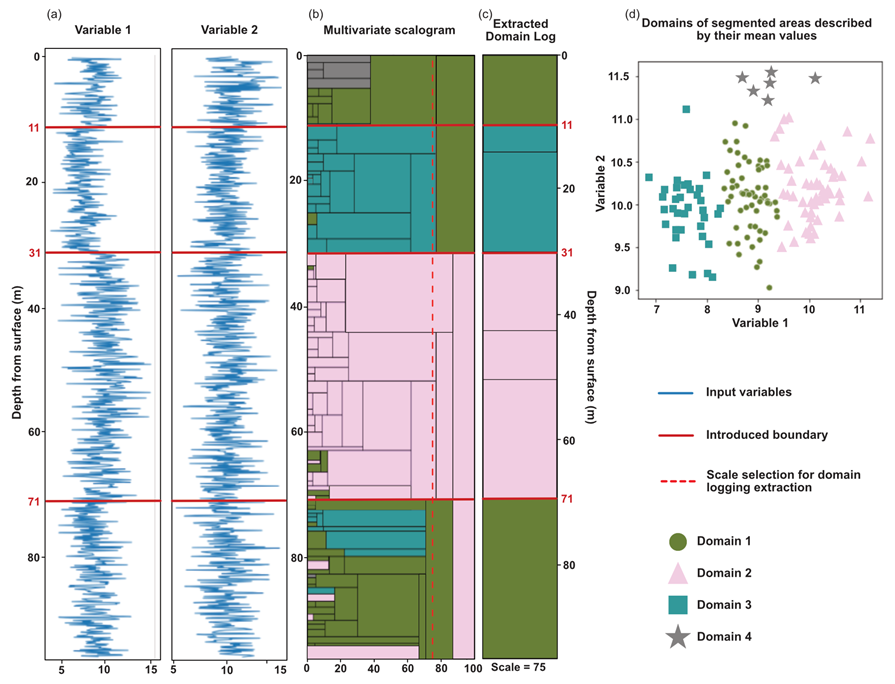
The synthetic dataset (Figure 3) simulates the log of two variables along a 96 m long borehole that intersect three (lithological) boundaries. The synthetic dataset concentrated in “Variable 1” and “Variable 2” (Figure 3e,f) was created by concatenating along depth four pairs of closely correlated random distribution with different lengths (Figure 3a–d). The pairs of random distributions have 110, 200, 400 and 250 samples, respectively, to simulate a sampling interval of 10 cm and lithological contacts at 11, 31 and 71 m depth. The random distributions were simulated mixing two white noise series from a normal (Gaussian) distribution center on five with a standard deviation of 1 by means of the Cholesky decomposition of a desired covariance matrix (using the Cholesky function from the linear algebra package linalg of the scipy open-source Python library). The code for the synthetic data generation has been included and can be found under the data availability statement.

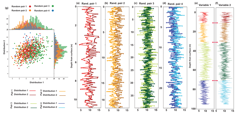
Figure 3.
Synthetic dataset. (a–d) Pairs of correlated variables with a simulated sampling rate of 10 cm along depth. The pairs-sets have different lengths with 110, 200, 400 and 250 samples, respectively. (e) Synthetic variable 1 created from the concatenation of the first random distribution from the four pairs. (f) Synthetic variable 2 created from the concatenation of the second random distribution from the four pairs. (g) Scatterplot of variable 2 against variable 1. The upper and right axes of the scatterplot show the marginal histograms.
2.1.2. Drill-Core Hyperspectral Multivariate Dataset
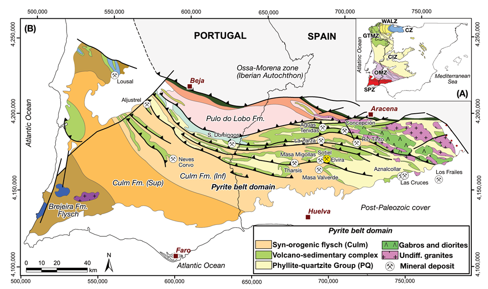
The multivariate data analyzed in this paper is derived from hyperspectral imaging of drill-core material from the Elvira case study, a shale-hosted polymetallic (Cu-Zn-Pb) pyrite-chalcopyrite rich massive sulfide deposit located at the southern Iberian Pyrite Belt (IPB) in south-west Spain (Figure 4). At Elvira, over 7 km of hyperspectral drill-core data were acquired along 80 boreholes and processed to obtain multivariate mineral abundance estimates [9]. We consider this dataset well suited to illustrate our approach for automated logging of multivariate data at the scale of an entire mineral deposit due to its complexity.

Figure 4.
(A) Iberian Massif Zones, CZ: Cantabrian Zone. WALZ: West Asturian-Leonese Zone. GTMZ: Galicia Tra’s os Montes Zone. CIZ: Central Iberian Zone. OMZ: Ossa Morena Zone. SPZ: South Portuguese Zone. (B) Geological scheme of the South Portuguese Zone with the location of main massive sulfide deposits in the IPB, highlighting in yellow the Elvira deposit. Map coordinate system: UTM Zone 29 ETRS 89. Modified from ([9,21,22]).
The multivariate input data contains mineral abundance estimations at millimeter resolution along the full length of entire boreholes. The predicted minerals include Muscovite, Biotite, Magnesium Chlorite, Iron Chlorite, Siderite, Ankerite, Iron Oxide, Quartz, Sulfides group 1 (grouping Pyrite, Arsenopyrite, Sphalerite and Galena) and Sulfides group 2 (grouping Chalcopyrite, Bornite, Covellite and Bournonite). A detailed explanation on the processing of the HSI from drill-cores to obtain the mineral abundances along boreholes is presented by [9] where a dictionary learning method [23] was applied as a supervised learning algorithm for estimating mineral quantities in drill-cores. The method is based on the co-registration between samples with high-resolution mineralogical information from scanning electron microscopy (SEM) data integrated with mineral liberation analysis (MLA) software and the hyperspectral data. This methodology allows the prediction of the mineral abundances for the entire drill-core hyperspectral dataset. The mineral abundance images are averaged across the width of the drill-core to obtain a single value per depth per variable (mineral) at a millimeter interval, to serve as mineral abundance logs. These will be fed to the proposed borehole segmentation algorithm. The results can be used for 3D modeling and are comparable to traditional core-logging techniques.
2.2. About the Continuous Wavelet Transform
Following [13], the continuous wavelet transform (CWT) is the integral of the product between a signal and a wavelet , i.e., their mathematical convolution. This operation is applied times, with , N being the number of data points, s a scale (as discussed below), and S the number of scales considered. The wavelet is both shifted and stretched along the borehole depth (hence parameterized by both a position index n and a scale index s), allowing us to extract information from the data at different scales. The convolution theorem allows us to do all convolutions simultaneously in the Fourier space by
where
is the Fourier transform of the signal , is the data spacing, is the frequency index, and
is the angular frequency. In the same way, the Fourier transform of the wavelet Equation (5) is given by Equation (6). Then, the inverse Fast Fourier transform is applied to to obtain the result.
The scale is related to the window size of the wavelet. A large-scale means a global view, and a small scale means a detailed view. The resolution is related to the frequency of the wavelet oscillation. The set of wavelet scales
are dependent on the data frequency , the smallest scale is set to two times the Nyquist frequency and therefore defines the smallest unit for the subsequent domains as the distance between two sample points. The subsequent scales are calculated as a fractional power of two with the fraction defined as the unit divided by the data frequency until J that determines the largest scale. The Gaussian function is perfectly local in both space and frequency and is indefinitely differentiable. Its order m derivative is
where is the gamma function. Both the Gaussian function and any of its derivatives are good choices for a wavelet, each highlighting different aspects of the signal.
2.3. Smoothing via CWT
In the first step (Figure 2b), a CWT is applied over the multivariate input data. To do so, the data are convolved with the Gaussian wavelet
i.e., corresponding to Equation (5) for . This process decomposes each input dataset along different scales and at the same time acts as a low-pass filter, slightly smoothing the high-frequency content of the data [24].
2.4. Moving-Window Principal Component Analysis
The decomposed data generated after the application of the first CWT along the scales is then fed to the moving-window principal component analysis (Figure 1 and Figure 2c,d). PCA [25] is the most commonly used technique for dimensionality reduction [26]. Through PCA of the multivariate dataset along the borehole we can detect changes in depth that are only expressed as changes in the correlation between variables, and could have remained undetectable if we analyzed each variable separately.
For some lithologies, the variability of mineral abundances can be very high, but for others the variability range can be very subtle. To avoid the range of variability between lithologies affecting the analysis and subtle changes being masked, the PCA analysis is performed in moving windows along the depth of the borehole, thus allowing for an analysis of local variability. To minimize the impact of the window size choice and the border effect that could be created between windows, a Gaussian notch filter is applied over the data within the window (Figure 1d). The Gaussian notch filter suppresses the data near the boundaries of the windows keeping the data values around the window center unmodified. The scores of the first principal component are then extracted for the three values at the center of the window to avoid border effects. The window is then moved onward by the three positions and the process is repeated until the window has moved through all the data along the borehole. Similarly, in order to prevent border effects at the outer edges of the dataset, the data are padded at the extremes with a mirror image of the data. It is important to mention that when calculating the PCA in specific window (w), the first eigenvector is defined only up to its direction, i.e., the sign of the loadings can change, thus inducing flips in the sequence of principal component scores. Therefore, to remove such flips, we enforce that the eigenvectors of two consecutive windows and have similar senses, i.e., that the scalar product . If this condition is not satisfied, we revert the sign of both the loadings and its corresponding scores.
After this process, we obtain as a result the first component of the moving-window PCA along the depth of the borehole and for each scale (Figure 1e).
2.5. Multivariate Segmentation Method
Another CWT is applied using the local first principal components for each scale that were obtained in the previous step as input data (Figure 1e), this time convolving the data with a boundary-detection wavelet: the first derivative of the Gaussian
Equation (8) can be obtained by Equation (5) with . As has been shown in previous studies [11,27], using this wavelet has two advantages: (i) the result will be zero at inflection points, and (ii) the zero-crossing value can be traced up to the smallest scale, which corresponds to the true location of the edge. At this stage (Figure 2h–j), the data can be considered to be univariate and therefore a scalogram can be calculated from the contour map following standard procedures (e.g., Hill et al., 2020 [16]). The borders extracted from the resulting contour map are tagged with two properties: (i) the position in depth; and (ii) the strength of this contact as a function of its continuity across scales and the steepness of its corresponding contour line. From this border dataset, the scalogram map is derived, presenting the segmentation of the borehole in a multi-scale framework (Figure 1k and Figure 2).
2.6. Unsupervised Domaining
The scalogram provides a spatial segmentation of the multivariate data at different scales, i.e., a grouping of samples per variable. In order to use this dataset as an input in a classification algorithm, a single value or a set of values has to be assigned to each segmented section. In this case, we selected the mean value per variable because it is a good representative descriptor of each segment, but the description of the group may also incorporate values such as the geometric mean per group, the vector of medians per group, parameters from a fitted variogram e.g., sill and range [28], or any other statistical descriptor of the variables on each segment. The mean vector on each segment is then used as an input for the linkage agglomerative clustering algorithm using the scipy library. We selected this algorithm over others because its hierarchical classification structure resembles the segmentation structure of the proposed method. This algorithm computes the distance between two clusters as the average of distances between points of each cluster Equation (9)
where and are the cardinalities of clusters u and v, and i and j are the indices of points belonging to cluster u, respectively, to cluster v. This method is also known as unweighted pair group method with arithmetic mean (UPGMA; [29]). This algorithm computed the distance between observations and in n-dimensional space as ’cityblock’ also known as the Manhattan distance, which is a special case of the Minkowski distance when ,
The algorithm begins with a forest of clusters that are combined by pairs based on a stepwise updated distance measure until one single cluster or root remains. Due to the geological multi-scale nature of the data, a hierarchical clustering algorithm of domains was chosen. This method produces geological domains in a similar way to a geological formation or lithostratigraphic unit description, obtaining larger domains as groups or supergroups that can be subdivided into smaller domains such as members and layers. Although there may be suitable alternatives to this approach, a comparison of machine-learning algorithms for classification is out of the scope of this study. The unsupervised domaining results in the classification of the multivariate scalogram segments in a pre-set number of domains. Finally, the multivariate mineral composition is used to generate geologically meaningful labels for each domain.
In the specific cases presented in this work, prior information guided the decision on the number of clusters, i.e., the number of synthetically generated intervals in the synthetic example guided us to select four clusters, and the number of lithologies described in the Elvira deposit in the real example guided us to select 18 clusters. In the case of not having any prior information, there are methodologies to estimate in advance the number of classes needed to capture the highest percentage of variability possible, i.e., elbow [30] or Log-Mean [31] methods.
3. Results
3.1. Results from Synthetic Data
The multivariate scalogram (Figure 2k) extracted from the synthetic dataset shows the segmentation of the borehole in depth at different scales. In the scalogram we can see that the number of segments increases towards the smaller scales. By using the mean values of both input variables for each obtained segment as input data for the unsupervised agglomerative clustering, we obtain a classification for all segments based on the input multivariate data (Figure 1m, Figure 2k and Figure 5b).
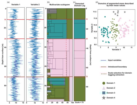
Figure 5.
Results of the synthetic dataset. (a) The two synthetic variables used as input data. (b) multivariate scalogram and domains based on unsupervised domaining. (c) Domain and segmentation data extracted at a scale of 75 shown as a logging file. (d) Scatterplot of compositional data for each segmented area described by the mean of their input variables.
The initial scalogram (Figure 2k) correctly identifies the three synthetically introduced contacts. Contacts produced due to the random nature of the data distributions are also identified. This can be demonstrated by applying the same segmentation algorithm to 100 realizations of the same model: the results reproduce the location of the true contacts at the same positions, while the other contacts strongly vary in location (Figure 2l).
3.2. Elvira Results
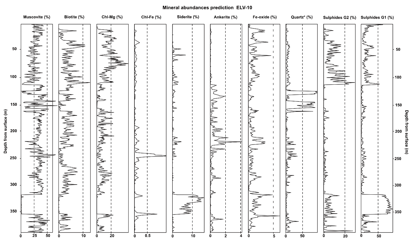
The Elvira deposit dataset is composed of 80 boreholes reaching an average depth of 400 m of which hyperspectral data were obtained from ca. 7 km of drill-core. The processing of the drill-core hyperspectral images produced a multivariate dataset as borehole logging files containing abundance predictions for ten minerals or mineral groups (described in Section 2.1.2) along the borehole sections with hyperspectral data. We use the multivariate dataset from the 80 boreholes (e.g., Figure 6) as input files for the method proposed in this paper aiming at obtaining geological domains that contain information on their mineralogical composition.
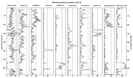
Figure 6.
Multivariate dataset of mineral abundances prediction for Muscovite, Biotite, Magnesium-rich Chlorite, Iron-rich Chlorite, Siderite, Ankerite, Iron Oxide, Quartz, Sulfide group 1 and Sulfide group 2 along the borehole ELV-10. For details on methodology see [9].
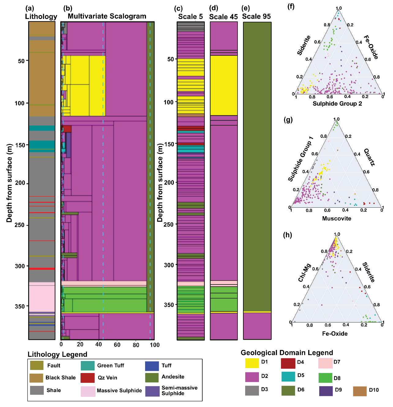
We first focus on the results of borehole ELV-10, which is considered representative for the entire set, before discussing the correlation between several boreholes. In general, the lithology of the ELV-10 borehole, according to the lithological log provided by the mining company, is made up of two black shale units hosting a massive sulfide lens. In this specific borehole, a green tuff layer is present at around 150 m depth and several faults and quartz veins can be observed along the entire length of the borehole. The lithological log (Figure 7a) is used as a qualitative means of validating our results. The multivariate scalogram graph for ELV-10 shows the depth from surface in meters on the vertical axis and the different spatial scales at which the data can be extracted on the horizontal axis. The scales are normalized between 0 and 100, but have a measurable spatial correspondence, i.e., in this case the scale of 0 is equivalent to 1 cm and the scale of 100 is equivalent to 290 m.
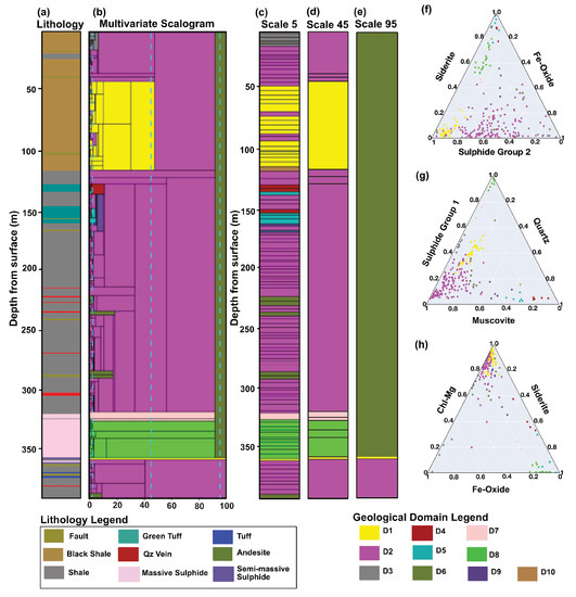
Figure 7.
Segmentation and domaining results for borehole ELV-10 of the Elvira deposit. (a) Lithological log provided by the mining company. (b) Multivariate scalogram and classification results. The three vertical dashed blue lines represent the scale corresponding to panels (c–e). (c–e) Geological domain classifications for the Elvira-10 borehole extracted from the scalogram at scales of 5, 45 and 95, respectively. (f–h) Ternary diagrams showing the average composition of domains in the multivariate scalogram, based on the relative composition of: (f) siderite, iron oxide and sulfide group 2. (g) sulfide group 1, muscovite and quartz. (h) magnesium-rich chlorite, siderite and iron oxide.
From the ELV-10 results (Figure 7), three major lithologic contacts can be appreciated and traced to the larger scales in the multivariate scalogram. The first major contact is found at a depth of about 110 m and is described in the lithology log as a change in the composition of the black shale. The second and third major contacts are found at a depth around 315 and 360 m, respectively, and are described in the lithological column (Figure 7a) as the massive sulfide interval. To illustrate the advantages of the multi-scale properties of the results, geological domains are extracted at three different observation scales, i.e., 5, 45 and 95, which correspond to approximately 2, 40 and 190 m, respectively (Figure 7c–e). Depending on the chosen scale, we can describe the same borehole with different levels of detail. At the larger scales, we observe geological domains of hundreds of meters in apparent thickness and at the smaller scales we observe domains of centimeters to meters in size, but all scales represent the same borehole. Furthermore, due to the available compositional data, we can add a geologically meaningful label to each domain based on its mineralogical composition.
A total of 18 Domains were manually selected based on the a priori knowledge of the number of existing lithologies for the unsupervised classification of the 80 Elvira boreholes. The geological domain classification for ELV-10 resulted in the identification of ten domains within it, which can be discriminated by their mineralogical composition (Figure 7f–h). Six domains are associated with shales (D1, D2, D3, D6, D9 and D10), mainly differentiated by their muscovite content. Two domains correspond to the massive sulfide (D7 and D8). Two domains (D4 and D5) are associated with volcanic rocks. The average values of each mineral for each domain are given in Figure A1 of the appendices.
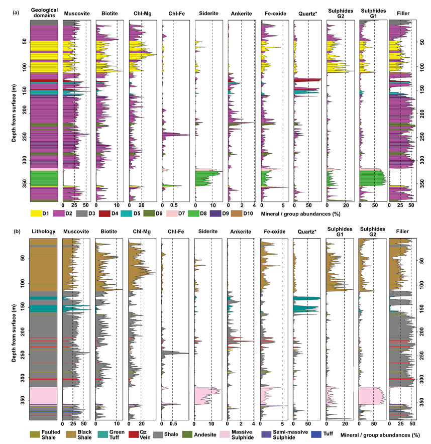
For validation and comparison of results against the lithological logs (Figure 8 and Figure 9), we selected the scalogram data at a scale of 5, which corresponds to two meters data aggregation along the borehole, producing results that visually most closely resembles the lithological logs. The filler is shown (Figure 8) to visualize the complete composition, when the filler shows low concentrations this implies that the composition is well described based on the sub-composition of the ten reported minerals. The values in this column are quite high, typically around 50% or more, since this filler also includes rock forming minerals. The filler column was not used as input data for any calculation (Figure 6).

Figure 8.
ELV-10 Borehole represented by the mineral abundance estimations of: Muscovite, Biotite, Magnesium-rich Chlorite, Iron-rich Chlorite, Siderite, Ankerite, Iron oxide, Quartz, Sulfides Group 1 and Sulfides Group 2 used as input data. The filler column comprises the sum of nine additional minerals (accessory and/or visible, near infrared and shortwave infrared spectrally inactive and accessory minerals). The first column in each sub figure guides the color scheme and represents (a) the lithology log from the mining company (b) the geological domains derived from the hyperspectral data by the proposed methodology extracted at a scale of 5.
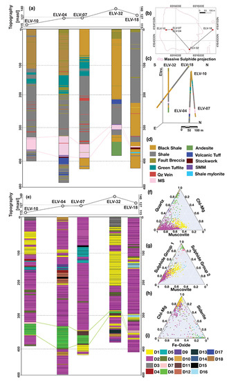
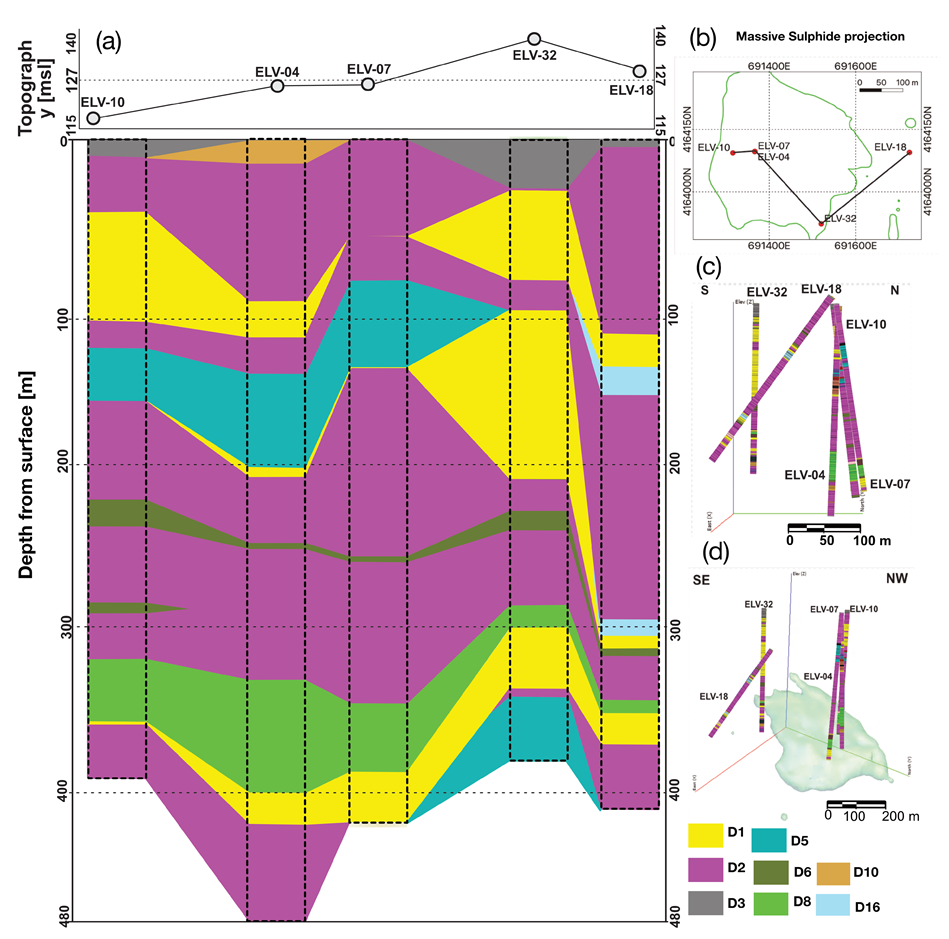
Figure 9.
E-W cross-section through the Elvira deposit showing ELV-10, ELV-04, ELV-07, ELV-32, ELV-18 boreholes. On top of the cross-section a topographic profile is shown. Continuous lines extrapolate horizontally the correlation of massive sulfide lithology/domains). (a) Boreholes with the color scheme guided by the lithological classification performed by the mine geologists. (b) Base map from the Elvira site, showing the cross-section profile and surface projection of the massive sulphide lens. (c) 3D visualisation of the boreholes utilized in the profile. (d) Lithological color legend. (e) Boreholes with the color scheme guided by the geological domains derived from the hyperspectral data by the proposed methodology extracted at a scale of 5. (f–h)Ternary diagrams showing composition of geological domains. (i) Geological domains color legend.
The interval around 340 m depth, logged as massive sulfides, is very well defined in the results as D8, a domain that compositionally corresponds to siderite massive sulfides (Figure 7a). In the upper part of the interval D8, another layer of contrasting composition (D7) is recognized. D7 is one of the three domains associated with massive sulfides and differs in its composition with D8 by having on average 8% more muscovite, 5% more magnesium-rich chlorite and 30% less sulfides group 1, which may be described as a semi-massive sulfide at the transition from the shale package to the massive sulfide, also showing a distinctive peak in iron-rich chlorite. Another unit (D3) is identified at the top of the borehole, which, based on its composition, is part of the shale package. This unit differs from the other shale domains based on a lower muscovite content, a 20% higher content in sulfide group1 minerals and a lower chlorite content.
D1 occurs at a depth of around 80 m and corresponds to the unit logged as black shales. In its composition, D1 is differentiated from the other shale units by a higher content of magnesium-rich chlorite, siderite and sulfides but also by a lower content of muscovite. The D2 domain is the most abundant in the borehole and correlates very well with the lithology described as shale. The light brown D10 domain is only visible in a small interval around 110 m depth, and it is also interpreted as shale. D10 can be differentiated from the other shale units by the higher muscovite values. D4 and D5 are found at depths of around 100 m and correlate well with a unit logged as green tuff. D4 and D5 are characterized by high abundances of Quartz* group minerals. Quartz by itself is a spectrally inactive mineral in the SWIR range of the electromagnetic spectrum, but the Quartz* group contains mixtures of fine-grained chlorite, muscovite, kaolinite and clays, which are intergrown with quartz [9] (Figure A2 Appendix B).
The D6 domain is characterized by relatively low concentrations of muscovite, high concentrations of ankerite and iron oxide when compared with the other shale domains. D6 corresponds to units logged as shales with quartz veins. However, based on the mineralogical composition of the domain, the quartz veins more likely correspond to carbonate veins (mixtures of ankerite and siderite). On the other hand, the D9 domain also corresponds to shales in some intervals characterized by the presence of quartz veins following the mine lithological description. Furthermore, the D9 domain stands out for its spatial characteristics which show extremely thin discontinuous intervals, which is consistent with the morphology of the quartz veins.
The method was applied to the 80 boreholes of the Elvira deposit. The borehole segmentation is run individually. However, the unsupervised domaining method (Section 2.5) was applied simultaneously to all boreholes, to ensure consistency between the clusters across all boreholes. A total of 18 domains were manually selected based on the number of existing lithologies as the number of clusters for the unsupervised domaining algorithm. For illustration purposes, we present a subset of this dataset consisting of five adjacent Elvira boreholes including ELV-10 (Figure 9). Geological domains were extracted at a scale of five, yielding results that visually resemble most closely the lithological logs, facilitating their qualitative visual comparison (Figure 9a). The lateral correlation of the geological domains between boreholes can be appreciated in the cross-section. The massive sulfide lens hosted in the shales is clearly identified, as is the lateral distribution of volcanic rocks. It is also possible to discriminate a layer of shales near surface (D3) whose difference in composition compared to the underlying shales may be explained by erosion and oxidation processes. In addition, there are domains in this cross-section that are only visible in one borehole such as D16 in ELV-18 or D13 in ELV-32. Based on its average composition, D16 is a shale enriched in biotite, iron-rich chlorite, iron oxides and sulfides. D13 is a domain interpreted as volcanic rock with the presence of ankerite. This is consistent with the mine geologist descriptions of andesite with carbonate veins.
4. Discussion
4.1. Benefits of a Multivariate Approach
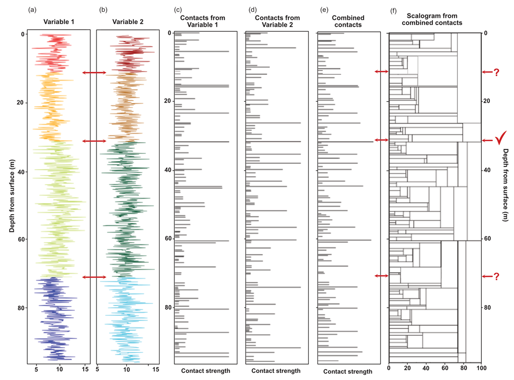
Our approach includes a moving-window principal component analysis that incorporates new insights from the correlation structure between multiple variables into the actual segmentation, taking full advantage of the multivariate nature of the data. We have shown in our synthetic example that datasets exhibiting changes in the correlation of variables can be correctly segmented using our approach. This is an innovation over state-of-the-art approaches that analyze each variable separately and combine the results in an additive way as a post-processing step (Figure 10). A univariate approach may be appropriate when only a single univariate dataset is available (such as a sample-based density log) but geological datasets, such as the presented hyperspectral imaging-derived mineral abundances, are inherently multivariate. For instance, a shale package may be distinguished based on the covariance between mica and chlorite, but both mica and chlorite may exhibit smooth changes across the actual contact, in which case univariate approaches may yield a poorly defined boundary or fail to detect it completely. By taking into account the multivariate nature of the data, our method improves the detection sensitivity of lithological contacts compared to the state-of-the-art tessellation approaches that are based on boundary extraction of each variable and subsequent combination (Figure 10).

Figure 10.
Results of the synthetic dataset using state-of-the-art methodology. (a,b) The two synthetic variables used as input data. The colour scheme of the variables in panels (a,b) is explained in Figure 3. (c) Contacts extracted from variable 1. (d) Contacts extracted from variable 2. (e) Combined contacts in the post-processing step. (f) Scalogram from combined contacts.
4.2. Support for Drill-Core Logging
The methodology presented in this paper is meant to support the core-logging process, which is performed on a visual basis in many cases. Hence, as a minimum requirement, the method should be able to reproduce the boundaries identified by a geologist. In this sense, the geological log, despite the inherent biases of this dataset, provides the ideal baseline reference to evaluate the fitness for purpose of the method. In order to compare them, we extracted the results at a scale that visually most closely resemble the lithological logs. Additionally, the number of clusters selected was driven by the number of lithological units described by the geologist. We have shown that the segmentation results of the Elvira data obtained with our approach are consistent with the lithological log (Figure 6, Figure 7, Figure 8 and Figure 9). In addition, it complements the information contained in the geological log as described in the following subsections.
4.2.1. Multi-Scale Results
The automatic logging results are multi-scale, thus allowing extraction of geological domains at any detail required for a specific objective, overcoming the limitation of having to choose a scale at the outset in traditional core-logging techniques. This allows more flexibility in typical exploration scenarios. Large-scale distribution of lithologies and the presence vs. absence of ore may be of highest importance for the mining company at initial stages of a project and knowledge of additional detail at a smaller scale (such as zonations of the ore body or stratigraphic marker horizons) may be required in a more advanced stage.
4.2.2. Hyperspectral Source for Multivariate Data
Hyperspectral imaging provides continuous mineralogical information along drill-cores, complementing analytical techniques such as geochemical assaying by means of X-ray fluorescence (XRF), modal mineralogy analysis with X-ray diffraction (XRD) and optical microscopy. Hyperspectral imaging can also complement high-resolution mineralogical analysis such as scanning electron microscopy (SEM) data integrated with mineral liberation analysis (MLA) software for mineral assemblage identification and quantification. The analytical techniques provide crucial mineralogical information, but they are expensive, time-consuming, destructive and usually performed sparsely, thus compromising the spatial representativity of the resulting data. Hyperspectral imaging provides continuous mineralogical information along drill-cores, and can provide a useful complement to these methods. Recent studies have shown that it is becoming more frequently used by the mining industry ([1,2,9,32,33,34,35]).
However, the lack of easily accessible tools is a major barrier for the widespread adoption of this technique. Moreover, there has been no clear methodology that implements drill-core hyperspectral imaging of an entire mineral deposit to contribute to 3D modeling of geological domains until now. With this work, we share an open-source Python tool that allows the application of the methodology described on multivariate datasets, presenting a solution to the aforementioned problems. The open-source nature of the approach offers several advantages: (i) wide use in academia and industry; (ii) easy and instantaneous access to the geoscientific community, catalyzing innovation; (iii) effective means of quality control and user feedback; (iv) enabling the user community to actively contribute to success; and (v) commercialization opportunities.
The automatic logging results presented in this paper are based on visible and infrared hyperspectral data that can identify mineralogical changes which may not be visually apparent. Moreover, the prediction of quartz content from VNIR-SWIR hyperspectral data can be done using as a proxy the identification of minerals associated with quartz from SEM-MLA samples (Figure A2 Appendix B). Nevertheless, the incorporation of long-wave infrared sensors will further improve the characterization of quartz together with pyroxene, olivine, garnet, feldspar, apatite and carbonates, among others. Comparing our results with the lithological description provided by the mining company in the Elvira deposit we classify seven different types of shales based on their composition (Figure A1 Appendix A). This is possibly due to the fact that the drill-core shale samples have a very fine grain size, with mineralogical changes invisible to the naked eye. In general the shales have a very uniform black color, making their discrimination difficult while performing the lithological logging. In the case of the sulfides, two types are described in the logs, a massive sulfide (MS) and a semi-massive sulfide (SMS) being differentiated by their density and texture. Based on the automated segmentation approach, we distinguish three geological domains associated with the massive sulfides (D7, D8 and D11), which can be differentiated based on their siderite, iron-rich chlorite, ankerite and iron oxide content. For lithologies associated with volcanic rocks, the geologists were able to recognize and identify green tuffits, volcanic tuff, breccias and andesites. However, from our results, eight geological domains associated with volcanic rocks are obtained (Figure A1 Appendix A). Another advantage of the presented method lies in the ability to differentiate between quartz and carbonates veins. In the lithological log, these veins are often mislabeled. On the other hand, there are lithological labels that are based on textural information, which are very easy to recognize with the naked eye but inconspicuous regarding mineral composition, as is the case of a mylonitic shale reported in the ELV-18 borehole, or the identification of fracture planes and faults. However, textural properties such as competence of a rock can be inferred based on the spatial distribution of a unit. For instance, as seen in Figure 7, domain D9 stands out from other domains for its spatial characteristics which show extremely thin discontinuous intervals.
4.2.3. Geologically Meaningful Domains
The automatic logging results provide geologically meaningful labels (Figure 9f–h) including a mineral composition for each domain. A domain described by its initial and final depth along the borehole and also described by its mineral composition can help geologists in the core-logging process to select appropriate and consistent labels. In some cases, the unsupervised domaining algorithm yields continuous segments along depth classified as the same geological domain where we observe one or several consecutive borders reported as horizontal black lines. As we can appreciate in Figure 7c, Figure 8 and Figure 9, the borehole segmentation algorithm is able to detect more inflection points from the data that translate into lithological contacts than the unsupervised classification algorithm. This apparent resolution difference between the segmentation algorithm and the unsupervised classification can be attributed to the fact that the segments found by the algorithm are then described with average values of their composition. As previously mentioned in Section 2.5, while there may be suitable alternatives to the selected unsupervised approach, a comparison of machine-learning algorithms for classification is out of the scope of this study.
4.3. Relevance for 3D Modeling
Several commercial software packages for 3D geomodeling allow users to incorporate hyperspectral data, which shows the relevance of hyperspectral data in the mining industry. However, currently, hyperspectral data can only be used for visualization purposes or brought in in the form of numerical univariate data, such as alteration indices (e.g., Lypaczewski et al., 2020 [7]). If multiple boreholes are processed at once, we observe a good consistency of the obtained domains across the boreholes, which is paramount for 3D geological modeling. Furthermore, the proposed methodology is both reproducible and objective, thus overcoming the subjectivity of traditional core-logging techniques. Traditional logging often produces inconsistencies across boreholes due to a variety of labels assigned by different geologists over time to the same geological units.
One of the advantages of this method is that it is not necessary to decide a scale to work with, providing the opportunity to obtain borehole units at any scale. Depending on the objective, we can describe all boreholes at a smaller or larger scale from centimeters to hundreds of meters. Multi-scale geological domains derived from drill-core hyperspectral images would be a new dataset to incorporate into 3D geological modeling workflows. In multi-scale modeling domains at larger scales could be used for regional modeling [36] and smaller scale domains could be used for modeling smaller areas in greater detail [37,38,39], in all cases aiming at spectrally differentiating lithological units that can be modeled in 3D.
A manual interpretation of the cross-section (Figure 9) has been included (Figure 11). In this case, the data for each borehole has been extracted on a scale of 45 which would correspond to approximately 40 m in length. The sketch shows the hierarchical behavior of the domains, and how units detected at larger scales can be used for a regional-scale model. The sketch is an oversimplification of the structural complexity of the area and the values between boreholes were manually interpolated. The intention of Figure 11 was not to represent the reality of the unknown but rather to illustrate the need for categorical data interpolation and uncertainty quantification in a 3D environment, while illustrating how multi-scale results can contribute to 3D modeling of mineral deposits.
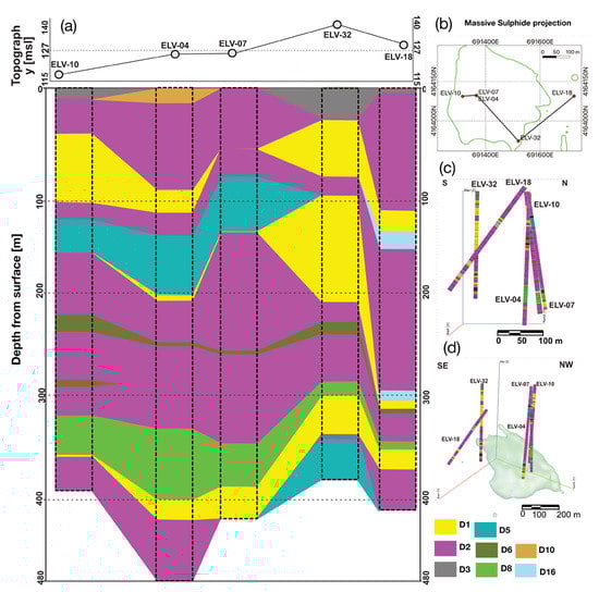
Figure 11.
(a) Manual interpretation of the E-W cross-section (Figure 9b) with geological domains derived from the hyperspectral data by the proposed methodology extracted at a scale of 45. (b) Base map from the Elvira site, showing the cross-section profile and surface projection of the massive sulphide lens. (c) 3D visualization of the boreholes utilized in the profile. (d) 3D visualization of the boreholes utilized in the profile together with an enveloping surface of the massive sulphide.
5. Conclusions and Outlook
There are geological changes that can only be detected when several variables are considered concomitantly. So far, state-of-the-art methods for borehole segmentation fail to register these changes. Traditional methods analyze each variable separately and combine the results in an additive way in a post-processing stage. This means that they are essentially univariate methods. We present a methodology that provides a solution for handling multivariate data in a novel way to automatically detect and extract lithological changes from the dependence structure between different variables. This approach allows a consistent segmentation across all boreholes of a deposit as multi-scale geologically meaningful domains.
The presented workflow is able to automatically extract multi-scale geological domains from a multivariate dataset, for instance derived from drill-core hyperspectral imaging. The resulting domains along boreholes are described by their mineralogical composition which produces geologically meaningful domains that can be modeled in 3D.
The performance of the method was demonstrated using a synthetic dataset. The multivariate nature of the data is truly exploited, accurately identifying lithological changes that would not be possible if the variables were analyzed independently.
The proposed methodology provides a useful tool to geologists to assist and complement the manual drill-core-logging process. In order to allow a large use, we provide the codes as open-source. The method is transferable to other deposit types and scalable to other areas. The method is not restricted to data derived from the hyperspectral images, it can also include multi-element geochemistry or geophysical borehole data e.g., borehole gamma ray, density, neutron porosity or electrical conductivity.
Author Contributions
Conceptualization, R.D.L.R., R.T.-D., M.K. and R.G.; methodology, R.D.L.R., R.T.-D., M.K. and R.G.; software, R.D.L.R.; validation, R.D.L.R., R.T.-D., M.K. and R.G.; formal analysis, R.D.L.R., R.T.-D., M.K. and R.G.; investigation, R.D.L.R.; data curation, R.D.L.R.; writing—original draft preparation, R.D.L.R.; writing—review and editing, R.D.L.R., M.K., R.T.-D. and R.G.; images, R.D.L.R.; supervision, R.T.-D., M.K. and R.G. All authors have read and agreed to the published version of the manuscript.
Funding
This study has been done within the framework of project NEXT (New Exploration Technologies, project webpage: http://www.new-exploration.tech) (accessed on 28 May 2022). This project has received funding from the European Union’s Horizon 2020 research and innovation programme under Grant Agreement No. 776804-H2020-SC5-2017.
Data Availability Statement
The Code and synthetic examples are available at: https://github.com/Robetodlr/Chunks (accessed on 28 May 2022). A module for multivariate synthetic dataset building is at the initial section of the code at: https://github.com/Robetodlr/Chunks (Accessed on 28 May 2022).
Acknowledgments
The authors wish to thank Juan Manuel Pons and Juan Carlos Videira from MATSA exploration department for providing the information and access to drill-cores, data and the Elvira deposit.
Conflicts of Interest
The authors declare no conflict of interest.
Appendix A
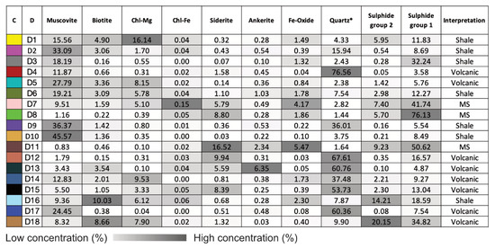
Figure A1.
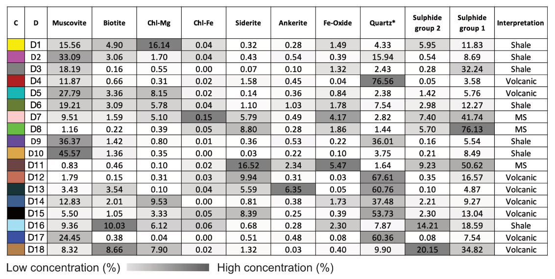
Unsupervised domain classification results, showing the domain color legend with average mineral abundances in percentage and the interpretation based on compositional data and knowledge integration. Massive sulfide (MS).
Figure A1.
Unsupervised domain classification results, showing the domain color legend with average mineral abundances in percentage and the interpretation based on compositional data and knowledge integration. Massive sulfide (MS).
Appendix B

Figure A2.
Mineral association to quartz from SEM-MLA samples.
Figure A2.
Mineral association to quartz from SEM-MLA samples.
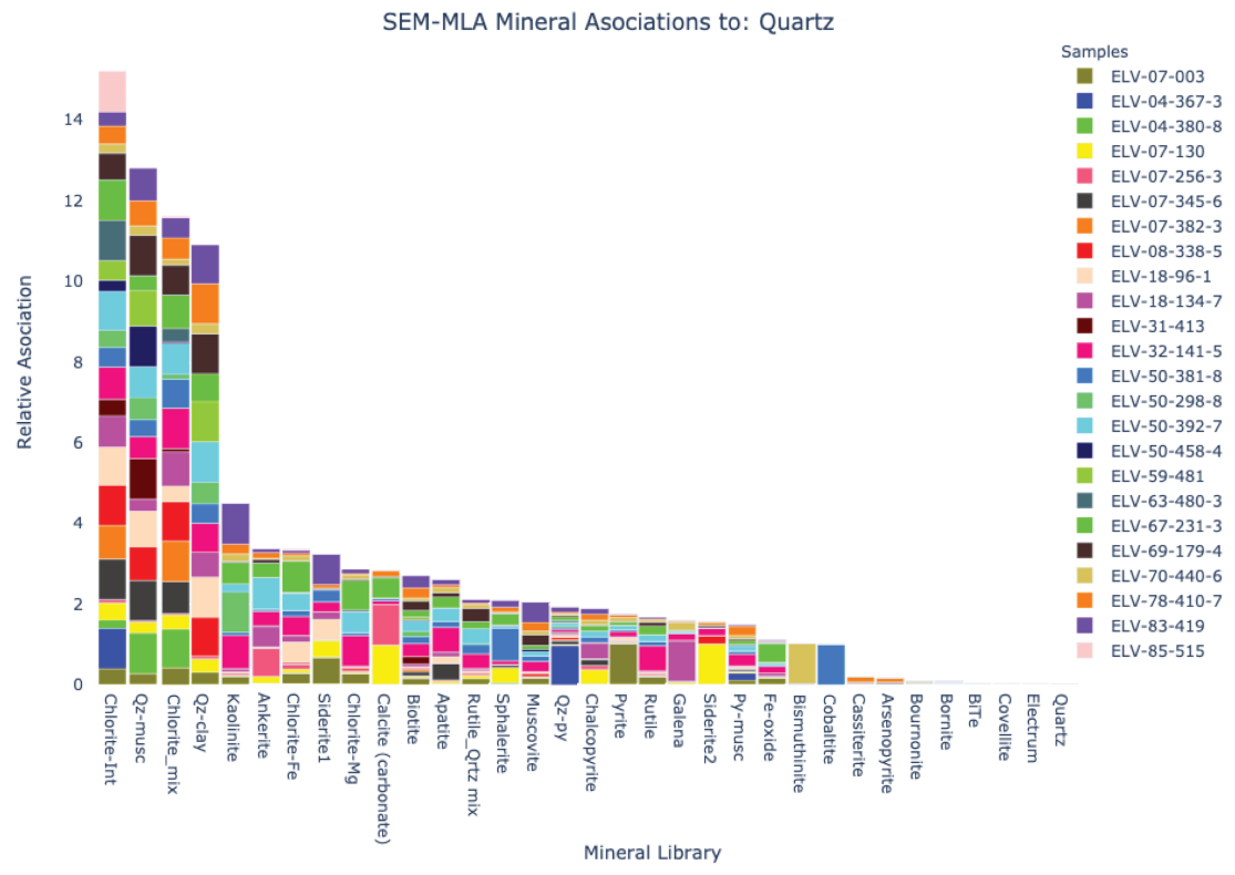
Based on 24 SEM-MLA samples from the Elvira deposit, a relative mineral association of Quartz was calculated. The association of a reference mineral A with another mineral B was calculated as the cumulative length of the contact between them normalized by the relative abundance of mineral B, both obtained from the same measurement with SEM-MLA [40].
This calculation is made for all minerals other than the reference mineral, in this case, quartz. The largest relative association obtained is with intermediate phases and mixtures of chlorite, muscovite, kaolinite and clays in general.
References
- Kruse, F.A. Identification and mapping of minerals in drill core using hyperspectral image analysis of infrared reflectance spectra. Int. J. Remote Sens. 1996, 17, 1623–1632. [Google Scholar] [CrossRef]
- Taylor, G.R. Mineral and lithology mapping of drill core pulps using visible and infrared spectrometry. Nat. Resour. Res. 2000, 9, 257–268. [Google Scholar] [CrossRef]
- Tappert, M.C.; Rivard, B.; Fulop, A.; Rogge, D.; Feng, J.; Tappert, R.; Stalder, R. Characterizing Kimberlite Dilution by Crustal Rocks at the Snap Lake Diamond Mine Hyperspectral Imagery Collected from Drill Core. Econ. Geol. 2015, 110, 1375–1387. [Google Scholar] [CrossRef] [Green Version]
- Mathieu, M.; Roy, R.; Launeau, P.; Cathelineau, M.; Quirt, D. Alteration mapping on drill cores using a HySpex SWIR-320m hyperspectral camera: Application to the exploration of an unconformity-related uranium deposit (Saskatchewan, Canada). J. Geochem. Explor. 2016, 172, 71–88. [Google Scholar] [CrossRef]
- Acosta, I.C.C.; Khodadadzadeh, M.; Tusa, L.; Ghamisi, P.; Gloaguen, R. A Machine learning framework for drill-core mineral mapping using hyperspectral and high-resolution mineralogical data fusion. IEEE J. Sel. Top. Appl. Earth Obs. Remote Sens. 2019, 12, 4829–4842. [Google Scholar] [CrossRef]
- Tusa, L.; Andreani, L.; Khodadadzadeh, M.; Contreras, C.; Ivascanu, P.; Gloaguen, R.; Gutzmer, J. Mineral mapping and vein detection in hyperspectral drill-core scans: Application to porphyry-type mineralization. Minerals 2019, 9, 122. [Google Scholar] [CrossRef] [Green Version]
- Lypaczewski, P.; Rivard, B.; Lesage, G.; Byrne, K.; D’angelo, M.; Lee, R.G. Characterization of mineralogy in the highland valley porphyry cu district using hyperspectral imaging, and potential applications. Minerals 2020, 10, 473. [Google Scholar] [CrossRef]
- Booysen, R.; Lorenz, S.; Thiele, S.T.; Fuchsloch, W.C.; Marais, T.; Nex, P.A.; Gloaguen, R. Accurate hyperspectral imaging of mineralised outcrops: An example from lithium-bearing pegmatites at Uis, Namibia. Remote Sens. Environ. 2022, 269, 112790. [Google Scholar] [CrossRef]
- De La Rosa, R.; Khodadadzadeh, M.; Tusa, L.; Kirsch, M.; Gisbert, G.; Tornos, F.; Tolosana-Delgado, R.; Gloaguen, R. Mineral quantification at deposit scale using drill-core hyperspectral data: A case study in the Iberian Pyrite Belt. Ore Geol. Rev. 2021, 139 Pt B, 104514. [Google Scholar] [CrossRef]
- Grossmann, A.; Morlet, J. Decomposition of Hardy Functions Into. SIAM J. Math. Anal. 1984, 15, 723–736. [Google Scholar] [CrossRef]
- Mallat, S. Zero-Crossings of a Wavelet Transform. IEEE Trans. Inf. Theory 1991, 37, 1019–1033. [Google Scholar] [CrossRef]
- Mallat, S.; Hwang, W.L. Singularity detection and processing with wavelets. IEEE Trans. Inf. Theory 1992, 38, 617–643. [Google Scholar] [CrossRef]
- Torrence, C.; Compo, G.P. A Practical Guide to Wavelet Analysis. Bull. Am. Meteorol. Soc. 1998, 79, 61–78. [Google Scholar] [CrossRef] [Green Version]
- Hill, E.J.; Robertson, J.; Uvarova, Y. Multiscale hierarchical domaining and compression of drill hole data. Comput. Geosci. 2015, 79, 47–57. [Google Scholar] [CrossRef]
- Feng, J.; Rivard, B.; Gallie, A.; Sanchez-Azofeifa, A. Rock type classification of drill core using continuous wavelet analysis applied to thermal infrared reflectance spectra. Int. J. Remote Sens. 2011, 32, 4489–4510. [Google Scholar] [CrossRef]
- Hill, E.J.; Pearce, M.A.; Stromberg, J.M. Improving Automated Geological Logging of Drill Holes by Incorporating Multiscale Spatial Methods. Math. Geosci. 2020, 53, 21–53. [Google Scholar] [CrossRef] [Green Version]
- Hill, E.J.; Fabris, A.; Uvarova, Y.; Tiddy, C. Improving geological logging of drill holes using geochemical data and data analytics for mineral exploration in the Gawler Ranges, South Australia. Aust. J. Earth Sci. 2021. [Google Scholar] [CrossRef]
- Zaitouny, A.; Ramanaidou, E.; Hill, J.; Walker, D.M.; Small, M. Objective Domain Boundaries Detection in New Caledonian Nickel Laterite from Spectra Using Quadrant Scan. Minerals 2022, 12, 49. [Google Scholar] [CrossRef]
- de Jong, S.; van der Meer, F. Remote Sensing Image Analysis: Including the Spatial Domain; Springer: Dordreecht, The Netherlands, 2006; p. 357. [Google Scholar]
- van der Meer, F.; Kopačková, V.; Koucká, L.; van der Werff, H.M.; van Ruitenbeek, F.J.; Bakker, W.H. Wavelength feature mapping as a proxy to mineral chemistry for investigating geologic systems: An example from the Rodalquilar epithermal system. Int. J. Appl. Earth Obs. Geoinf. 2018, 64, 237–248. [Google Scholar] [CrossRef]
- Tornos, F. Environment of formation and styles of volcanogenic massive sulfides: The Iberian Pyrite Belt. Ore Geol. Rev. 2006, 28, 259–307. [Google Scholar] [CrossRef]
- Martin-Izard, A.; Arias, D.; Arias, M.; Gumiel, P.; Sanderson, D.J.; Castañon, C.; Lavandeira, A.; Sanchez, J. A new 3D geological model and structural evolution of the world-class Rio Tinto VMS deposit, Iberian Pyrite Belt (Spain). Ore Geol. Rev. 2015, 71, 457–476. [Google Scholar] [CrossRef] [Green Version]
- Khodadadzadeh, M.; Gloaguen, R. Upscaling High-Resolution Mineralogical Analyses to Estimate Mineral Abundances in Drill Core Hyperspectral Data. In Proceedings of the International Geoscience and Remote Sensing Symposium (IGARSS), Yokohama, Japan, 28 July–2 August 2019; pp. 1845–1848. [Google Scholar] [CrossRef]
- Brigham, E.O. The Fast Fourier Transform and Its Applications by E. Oran Brigham; Prentice-Hall Inc.: Hoboken, NJ, USA, 1988; Volume 12, p. 448. [Google Scholar]
- Pearson, K. On lines and planes of closest fit to systems of points in space. Lond. Edinb. Dublin Philos. Mag. J. Sci. 1901, 2, 559–572. [Google Scholar] [CrossRef] [Green Version]
- Doventon, J. Geologic Log Analysis Using Computer Methods; The American Association of Petroleum Geologist: Lawrence, KS, USA, 1994; pp. 79–88. [Google Scholar]
- Witkin, A.P. Scale-Space Filtering. In Proceedings of the 8th International Joint Conferences on Artificial Intelligence, Karlsruhe, Germany, 8–12 August 1983; Volume 2, pp. 1019–1022. [Google Scholar] [CrossRef]
- Chilès, J.P.; Delfiner, P. Geostatistics Modeling Spatial Uncertainty, 2nd ed.; John Wiley & Sons, Inc.: Hoboken, NJ, USA, 2012; Number 2; p. 699. [Google Scholar]
- Sokal, R.R.; Michener, C.D. A Statistical Method for Evaluating Systematic Relationships; Harvard University: Cambridge, MA, USA, 1958; Volume 38, pp. 1409–1438. [Google Scholar]
- Thorndike, R.L. Who belongs in the family? Psychometrika 1953, 18, 267–276. [Google Scholar] [CrossRef]
- Fritz, M.; Behringer, M.; Schwarz, H. LOG-means: Efficiently estimating the number of clusters in large datasets. Proc. Vldb Endow. 2020, 13, 2118–2131. [Google Scholar] [CrossRef]
- Tappert, M.; Rivard, B.; Giles, D.; Tappert, R.; Mauger, A. Automated drill core logging using visible and near-infrared reflectance spectroscopy: A case study from the Olympic Dam Iocg deposit, South Australia. Econ. Geol. 2011, 106, 289–296. [Google Scholar] [CrossRef]
- Littlefield, E.; Calvin, W.; Stelling, P.; Kent, T. Reflectance spectroscopy as a drill core logging technique: An example using core from the Akutan. Trans.–Geotherm. Resour. Counc. 2012, 36, 1281–1283. [Google Scholar]
- Kruse, F.A.; Bedell, R.L.; Taranik, J.V.; Peppin, W.A.; Weatherbee, O.; Calvin, W.M. Mapping alteration minerals at prospect, outcrop and drill core scales using imaging spectrometry. Int. J. Remote Sens. 2012, 33, 1780–1798. [Google Scholar] [CrossRef] [Green Version]
- Calvin, W.M.; Pace, E.L. Mapping alteration in geothermal drill core using a field portable spectroradiometer. Geothermics 2016, 61, 12–23. [Google Scholar] [CrossRef] [Green Version]
- Cowan, E.J. Deposit-scale structural architecture of the Sigma-Lamaque gold deposit, Canada—Insights from a newly proposed 3D method for assessing structural controls from drill hole data. Miner. Depos. 2020, 55, 217–240. [Google Scholar] [CrossRef] [Green Version]
- Jones, R.R.; McCaffrey, K.J.; Clegg, P.; Wilson, R.W.; Holliman, N.S.; Holdsworth, R.E.; Imber, J.; Waggott, S. Integration of regional to outcrop digital data: 3D visualisation of multi-scale geological models. Comput. Geosci. 2009, 35, 4–18. [Google Scholar] [CrossRef]
- Dai, H.; Liu, Z.; Hu, J. Multi-scale 3D geological digital representation and modeling method based on octree algorithm. In Proceedings of the 2010 6th International Conference on Wireless Communications, Networking and Mobile Computing, WiCOM 2010, Chengdu, China, 23–25 September 2010; Number c. pp. 6–8. [Google Scholar] [CrossRef]
- Xiong, Z.; Guo, J.; Xia, Y.; Lu, H.; Wang, M.; Shi, S. A 3D Multi-scale geology modeling method for tunnel engineering risk assessment. Tunn. Undergr. Space Technol. 2018, 73, 71–81. [Google Scholar] [CrossRef]
- Heinig, T.; Bachmann, K.; Tolosana-Delgado, R.; Van Den Boogaart, G.; Gutzmer, J. Monitoring gravitational and particle shape settling effects on MLA sampling preparation. In Proceedings of the IAMG 2015—17th Annual Conference of the International Association for Mathematical Geosciences, Freiberg, Germany, 5–13 September 2015; pp. 200–206. [Google Scholar]

Publisher’s Note: MDPI stays neutral with regard to jurisdictional claims in published maps and institutional affiliations. |
© 2022 by the authors. Licensee MDPI, Basel, Switzerland. This article is an open access article distributed under the terms and conditions of the Creative Commons Attribution (CC BY) license (https://creativecommons.org/licenses/by/4.0/).