Using Open Vector-Based Spatial Data to Create Semantic Datasets for Building Segmentation for Raster Data

Abstract

With increasing access to open spatial data, it is possible to improve the quality of analyses carried out in the preliminary stages of the investment process. The extraction of buildings from raster data is an important process, especially for urban, planning and environmental studies. It allows, after processing, to represent buildings registered on a given image, e.g., in a vector format. With an actual image it is possible to obtain current information on the location of buildings in a defined area. At the same time, in recent years, there has been huge progress in the use of machine learning algorithms for object identification purposes. In particular, the semantic segmentation algorithms of deep convolutional neural networks which are based on the extraction of features from an image by means of masking have proven themselves here. The main problem with the application of semantic segmentation is the limited availability of masks, i.e., labelled data for training the network. Creating datasets based on manual labelling of data is a tedious, time consuming and capital-intensive process. Furthermore, any errors may be reflected in later analysis results. Therefore, this paper aims to show how to automate the process of data labelling of cadastral data from open spatial databases using convolutional neural networks, and to identify and extract buildings from high resolution orthophotomaps based on this data. The conducted research has shown that automatic feature extraction using semantic ML segmentation on the basis of data from open spatial databases is possible and can provide adequate quality of results.

1. Introduction

Increasing access to open spatial data and the development of machine learning algorithms mean that information can be extracted accurately from satellite and aerial imagery. On this basis, it is possible to determine the location of objects more precisely at the early stages of urban, planning and environmental analyses.

Information extraction can take place at different levels of complexity. The result is mainly dependent on the input data, the object of analysis and the algorithm used. Open spatial data are currently an increasingly important source of information in various areas of the economy. Their numbers are enormous and the amount of disk space they occupy is growing every day [1]. However, the use of such data requires processing it for specific applications. For several years, solutions based on deep neural networks have been increasingly popular. As a result, it is possible to classify, detect or segment objects, for example, from open raster data.

The application of semantic segmentation to geospatial data gives satisfactory results for: the extraction of objects, such as buildings [2,3,4,5,6,7,8,9]; roads [10,11]; the assessment of damage due to natural disasters [12]; or during population density assessment [13]. The problem with semantic segmentation is the small amount of publicly available labelled data that can be used to train the network. Creating datasets based on manual labelling of data is a tedious, time-consuming and capital-intensive process [14,15,16], and any errors can affect the results of the analysis. These problems motivate the search for solutions to automate the creation of masks for semantic segmentation from raster data (e.g., orthophotos), including those based on open vector spatial data [3]. Compared to our approach, existing works do not use mostly accurate and publicly available cadastral data or use less accurate data (raster with larger terrain pixel) as, for example, in Inria Dataset [17], and are not as flexible. In our approach, we can use data from different areas and create diverse datasets, as will be shown later in the paper.

Raster-based open spatial data can be divided into global and local (national). Global data are mainly remote sensing data acquired from satellites. The European Space Agency’s Sentinel-2 mission allows the free acquisition of raster data which contains information not only on RGB channels, but also other spectral channels. The advantage of these type of data is that they are updated every few days, whereas the disadvantage is their spatial resolution. Therefore, they are most often used for macro analyses (also using deep neural networks) for segmentation, e.g., for fire impact assessment [18] and land cover analysis [19,20,21]. On the other hand, segmentation of individual buildings for open data is not possible—it would be necessary to use commercial data, whose spatial resolution is much better, such as in [22,23].

Raster local (national) data are the data made available by individual national institutions that operate (acquire, store or make available) geospatial data; for example, in Poland, this role is fulfilled by the Central Office of Geodesy and Cartography (GUGiK). The registers provide access to various resources: orthophotomaps with a resolution of up to 5 cm; vector layers of The Land and Building Register (EGiB); The Topographic Objects Database (BDOT10k) for a scale of 1:10,000; Digital Terrain Models and Digital Surface Models; LiDAR data, and others. The main problem of the data is the verification of their validity, as they are usually created every certain time unit (years). The LandCover dataset [24] which is used for land use segmentation on the basis of orthophotomaps was created on the basis of data that was made available by GUGiK. In various European countries, similar data are provided by institutions analogous to the GUGiK.

Similar to raster-based data, vector-based open spatial data can be divided into global and national scale. Open Street Map (OSM) is a global project that aims to create a free, editable map of the world. It is built by users and made available under an open-content licence. Segmentation using OSM has been carried out, among others, in [3,12].

Open vector data of national scale, similar to raster data, are made available by national institutions operating geospatial data. In Poland, such a resource is, for example, information on The Land and Building Register (EGiB) which is part of the cadastral database. The approach using open vector data for dataset creation was used by among others [9]. However, there the dataset is not described in detail the type of input data and what the problems of this dataset might have been are not described).

The problem of automatic labelling or using data resources that cannot be clearly labelled is not a simple one. Most often these data are not suitable to be directly labelled and must be processed through a transformation and rasterization process.

The aim of this paper is to present the results of work on verifying the possibility of using open vector spatial data as labels for the process of training convolutional neural networks and solving the task of the semantic segmentation of buildings for raster data. The paper uses fully open data that is available in the authors’ country of residence—Poland—from the following databases: cadastral data of The Land and Building Register (EGiB) for a selected location in Poland and orthophotomaps taken from aerial photographs, made available by the Central Office of Geodesy and Cartography in Poland.

The motivation for the research was to verify the possibility of simplifying the tedious and time-consuming process of data labelling. The research goal was to verify the possibility of creating machine learning datasets based on the use of open spatial data. In addition, the research verified the impact of using available popular network architectures for solving semantic segmentation problems, i.e., UNET and DeepLabV3+, in order to obtain an algorithm that was characterised by the highest possible reliability. The algorithm was also verified in terms of differences in identification of buildings for different orthophoto terrain pixels.

The main novelty with respect to the other work is the verification of the use of fully open, accurate data to segment buildings from aerial photographs. This provides the opportunity to create large, diverse datasets that are flexible and contain multiple patterns. Additionally, the data used are characterised by high accuracy (low pixel resolution and high accuracy of vector data), where in the other works the data are far less accurate. In addition, the proposed algorithm allows for the creation of huge learning datasets from cadastral data, which are currently made publicly available by many European countries. The algorithms that were developed as a result of the work can be used, among others, for:

• Verification of the state of the cadastral databases in order to identify unpermitted buildings;
• Verification of the actual state of an area in the initial phase of an infrastructural investment process for a more reliable cost assessment;
• Mapping of buildings for unmapped areas;
• Verification of the validity of open building databases.

The structure of the article is as follows. The Section 1 introduces the topic and describes related works. The Section 2 describes the dataset that was used, discusses the issues related to it and the data pre-processing. The Section 3 discusses the network architectures that were used and presents the algorithm and processing strategies that produced the final result. The Section 4 presents the obtained results, which are then analysed—both statistically and visually. In addition, a discussion of the results is presented in this section. The paper concludes with a summary and conclusions of the conducted research in the Section 5.

2. Study Area and Datasets

2.1. Open Spatial Data

This paper focuses on the possibility of using open spatial data using the example of data that is available in the authors’ country of residence, Poland. This section is a characterisation of open spatial data available in Poland which were used in the research, i.e., orthophotomaps and cadastral data—The Land and Building Register (hereinafter: EGiB). The use of OpenStreetMap (hereinafter: OSM) resource was also considered, but it was ultimately abandoned for reasons described in the next section.

Open spatial data in Poland are available on the basis of individual laws and European regulations concerning spatial information infrastructure, including the Inspire Directive [25]. The data are made available through the Geoportal [26] which is maintained by the Head Office of Geodesy and Cartography, or through individual local government units. The list of maintained resources is available at [27]. These units are obliged to maintain and make available free of charge (usually in an incomplete form for reasons of personal data protection and legal interests) geodetic resources, including those concerning the cadastre—EGiB. However, these resources are currently under development and are not yet available nationwide in a downloadable form.

The resources are maintained in various coordinate systems. Most often, data from the national dataset (e.g., orthophotomaps) are provided in the PL1992 system (EPSG 2180), while data from local government units (e.g., EGiB) are provided in the PL2000 system (EPSG 2176-2179—depending on the zone).

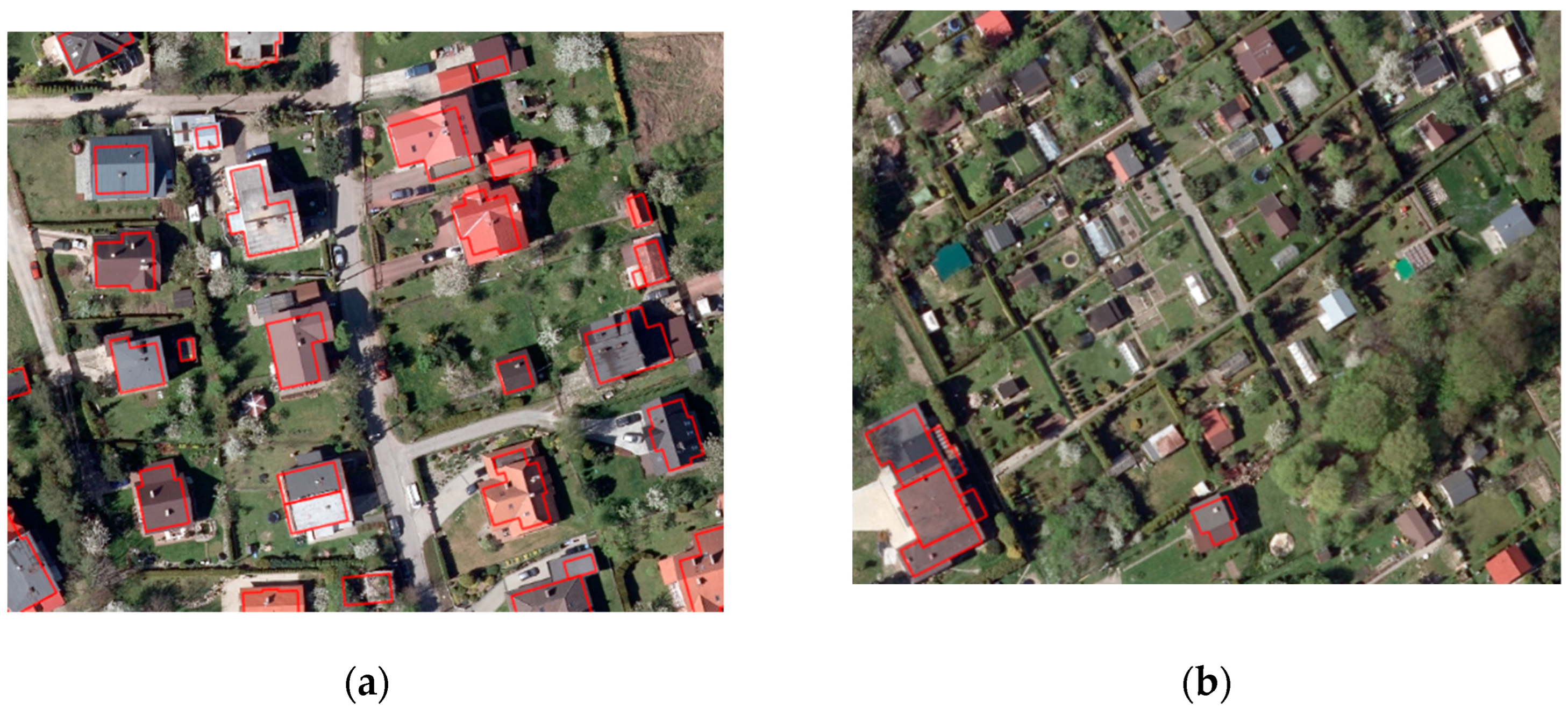
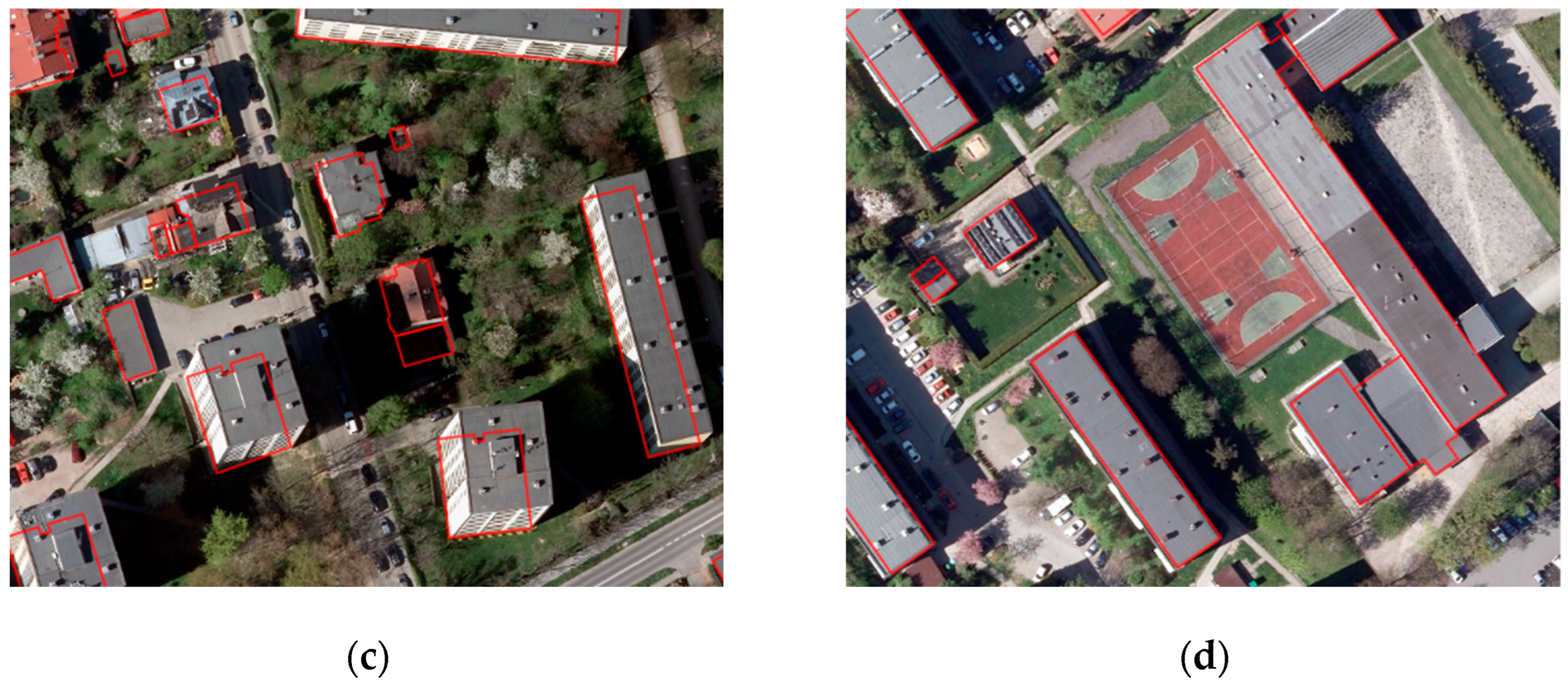
2.2. Selection of Study Areas

The following criteria were used to select the area for further analysis:

• Urban area;
• Architecture varying in terms of time of construction (historic buildings, often with more complicated architecture and contours, and modern buildings with simpler shapes);
• Architecture varying in terms of use (residential, industrial, public buildings, etc.);
• Building density and diversity;
• Availability of actual orthophotomap (max. up to one year back) with terrain pixel of max. 10 cm;
• Availability of data from the cadastral vector database: The Land and Building Register (EGiB).

In response to these criteria, the city of Bielsko-Biała in southern Poland in the Silesian Voivodeship was selected for further analysis. It is a city with diverse architecture, consisting of both older buildings and districts with modern buildings. Additionally, the city contains industrial areas with factories or large warehouses. In terms of building density and diversity, the city is characterised by a centre with compact buildings and, within a radius of about one kilometre, a less dense suburban area. Both an orthophotomap (dated 2021, with a maximum terrain pixel of 10 cm) and data from EGiB database were available for the city.

At the stage of selecting data sources, the use of two vector data resources, i.e., EGiB and OSM, was considered. The selection of the resource for further analysis was based on the verification of the actuality of these resources in relation to the orthophotomap of 2021, obtained from the Polish Geoportal [26]. Figure 1 shows the comparison between EGiB and OSM data. In green, the common parts of both resources are presented, in yellow the objects that are only in the EGiB database, while in red the elements that are only in the OSM database.

The analysis showed that the main problem of OSM resources is that they are outdated. Data from EGiB are more up-to-date, more accurate and complete and have no artefacts. Examples are presented in Figure 1 and—depending on the type of problem—are marked as the following areas:

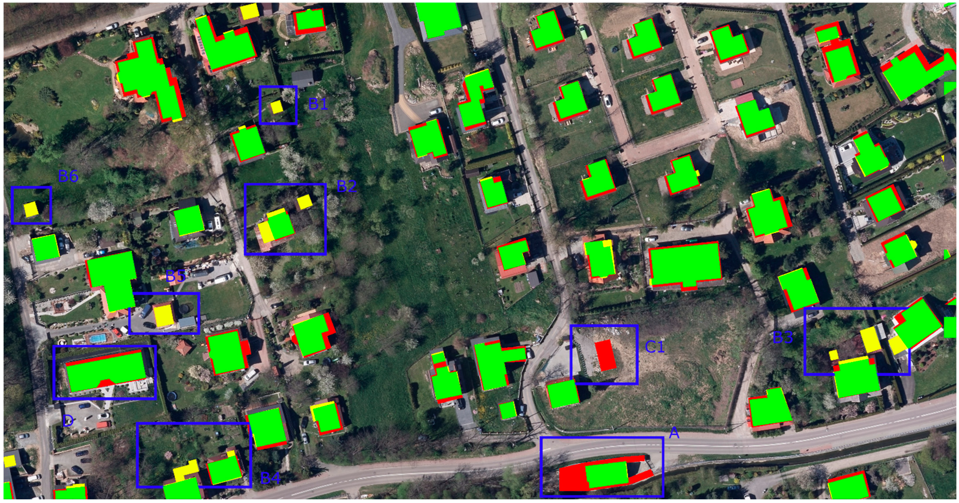
• Area A—incorrectly determined outline of the building in the OSM database (the car park located next to the building was included in the building projection);
• Areas B1, B2, B3, B4, B5, B6—no buildings that actually exist in the OSM database;
• Area C1—presence in the OSM database of buildings which in fact do not exist;
• Area D—generalisation of building outline (simplification of building outline shape).

Since all the indicated problems may result in a much lower accuracy of the network and the wrong extraction of buildings, in further works it was decided to use only the EGiB database.

Before proceeding to further work, the input data from the EGiB database were analysed in relation to the orthophotomap. This comparison was aimed at identifying possible errors that could affect the results of the algorithm and, consequently, the possibility of extracting buildings.

Firstly, the obvious problem that was identified was that the mask outline of the dataset followed the wall outline, not the roof outline. This was due to the specificity of the EGiB database, which contains the vertices of the wall points. The applied roof eaves and other elements intended to protect the objects against, for example, the degrading activity of rainwater, increased the building outline. The problem is illustrated in Figure 2a. However, it was considered that the problem could be omitted given the purpose of the study, i.e., to identify the existence of objects with an approximate outline rather than to identify their exact outline.

For the same reason, the problem caused by the available orthophotomap not being a true orthophotomap [28] and containing radial displacements which are particularly visible for tall objects was also omitted. A true orthophotomap is slowly being made available by the Central Office of Geodesy and Cartography. As of the writing of this article, i.e., the end of February 2022, the EGiB database was not available for the area that was subject to the creation of this type of product, and therefore it had to be excluded as a candidate for analysis. However, in each case, the building from the EGiB database is located within the outline boundaries of the objects with the orthophotomap. This problem is presented in Figure 2c.

In addition, the EGiB database does not consider objects that are: not permanently connected to the ground; additional elements of buildings such as terraces, summer cottages, farmhouses, outbuildings or allotments. For this reason, the database is incomplete. Therefore, in the process of data preprocessing it was decided not to consider the objects that are not included in the EGiB database. The problem is presented in Figure 2b.

Figure 2d shows an area that is not subject to any of the problems described above. This is also the case for most of the area to be analysed, so it was decided to check the possibilities described above for the segmentation of the buildings.

2.3. Data Preprocessing

Publicly available datasets for object segmentation are most often created manually based on vector data from OSM or corrected manually based on publicly available building outlines. Datasets are also created based on commercially acquired data. However, our aim was to create a dataset completely free of charge.

The input orthophoto data included six images in. GTiff format with a ground pixel resolution of 10 cm. The areas that were selected for analysis were diverse in terms of architecture and building density. The dimensions of each image in pixels were 22,477 × 23,162, and in metres 2247.7 m × 2316.2 m. The area of analysis therefore covered an area of over 31 square kilometres. In the study area there were 21,010 buildings in vector format, available in the EGiB database.

From the input data, which consisted of orthophotomaps and vector data from EGiB, two datasets were created according to the algorithm presented in Figure 3: the first one for the input pixel with the terrain pixel of 10 cm and the second one with the terrain pixel of 50 cm. The second dataset was created by resampling data from the first, main dataset. The algorithm was programmed using the Python language and the gdal, ogr, opencv and patchify libraries. Different terrain pixels from the input data were used to compare the performance of the algorithms with respect to the size of the terrain pixels and to evaluate the possibility of segmenting buildings on these pixels.

The data were split into smaller images that were suitable for neural networks. This is a recommended action as it reduces the computing power required. Then, only those images where buildings were present were selected.

The first dataset contained 6365 images with dimensions: width—512, height—512, number of channels—3 (RGB colours) and corresponding labels in the form of binary image masks (1—buildings, 0—background) that were obtained as a result of rasterization. The data were divided into training set—80% of data, validation set—10% and testing set—10%. They contained, respectively, 5092 training images, 636 validation images and 637 test images. Similar work was carried out with the second dataset with a larger terrain pixel. The division of the large images into smaller images resulted in 1263 images with dimensions: width—256, height—256, number of channels—3 (RGB colours) and corresponding labels in the form of binary image masks (1—buildings, 0—background) that were obtained by rasterization. The data were divided in the same ratio as the first dataset and in this way 1010 training images, 126 validation images and 127 test images were obtained. A summary of both datasets is shown below in

Table 1. Summary of created datasets.

Resolution [m]	Image Size [pix]	Image Size [m]	Training Images Number	Validation Images Number	Test Images Number
0.1	512 × 512 × 3	51.2 × 51.2	5092	636	637
0.5	256 × 256 × 3	128.0 × 128.0	1010	126	127

. Figure 4 shows raster data visualisations of the two datasets for visual comparison of the datasets. Clearly, more blurring is seen for the larger ground pixel, so a worse performance of the proposed architectures for this dataset is to be expected. The datasets have been made available on a repository [29] via the GitHub platform.

We are aware that somewhat false ground-truth data (containing the errors mentioned in the previous section) were used for testing. Testing of the algorithm with manually produced data (true ground-truth) is planned in future work. We anticipate that this may affect the accurate extraction of building edges, but as mentioned, our aim is to test the feasibility of using fully open data for building segmentation.

3. Materials and Methods

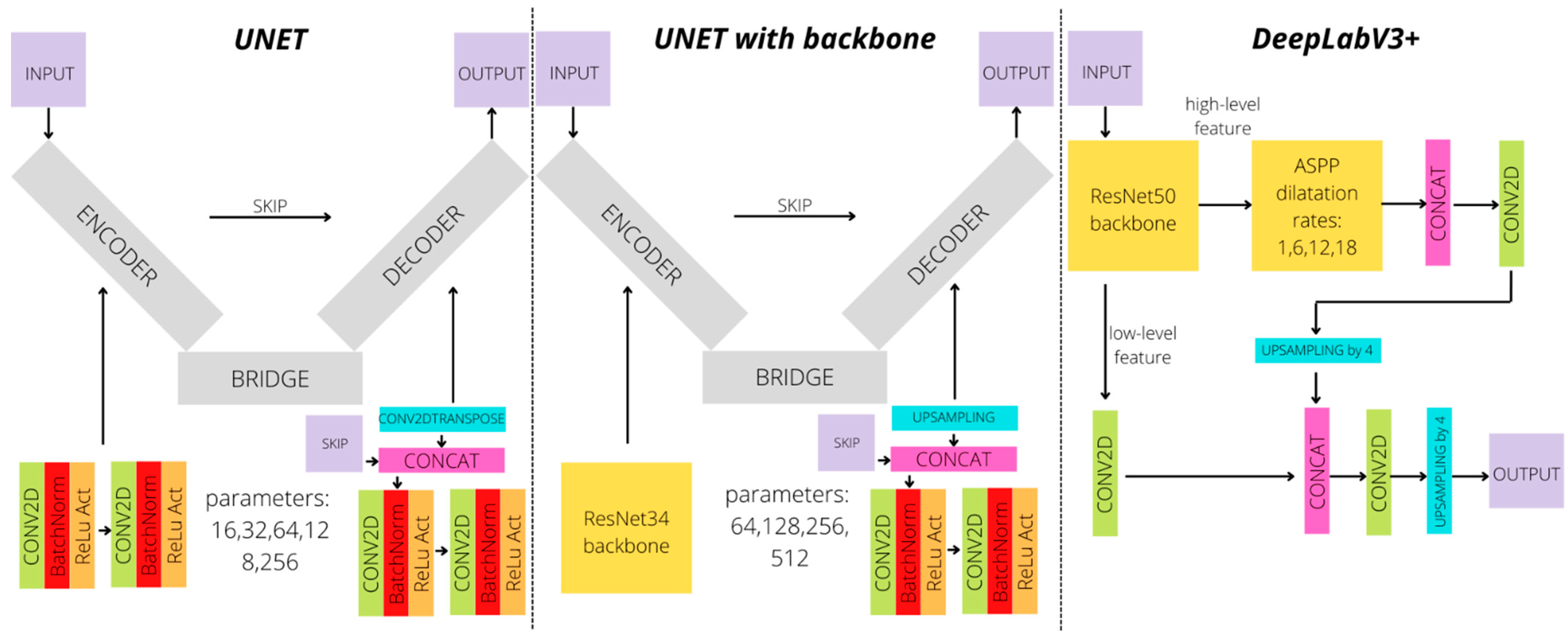
3.1. Semantic Image Segmentation Architectures

Currently, the most commonly used network architectures for image segmentation tasks are different variations of UNET and DeepLab. SegNet [30,31] and PSPNet [32] are also used, however, their use for further analyses was rejected because they are usually less efficient. Choosing the most optimal architecture was not the aim of the paper, but we would like to describe them briefly.

UNET consists of two main segments: the encoder and the decoder. The encoder at the initial stage consists of convolutional blocks, at the ends of which a pooling layer is implemented to reduce dimensionality. After moving to the dimensionality change pointbridge, dimensionality is increased by deconvolution or upsampling. Additionally, block information from the encoder is skipped and concatenated, followed by a convolution block. The operation is repeated until the input dimensions are obtained, where a predicted mask is obtained using the final convolution layer with the appropriate activation function [33]. The above description is the foundation of the network. In the years following the emergence of UNET network, various research teams have tried to modify it so that it provides even better results for different applications. Such an approach can be the use of DeepUNET [34], DeepResUNET [5,8] or combining UNET with solutions such as ASPP (Atrous Spatial Pyramid Pooling) [10]. From the point of view of information extraction from aerial images or satellite imagery, the results presented in [35,36] are particularly interesting. The obtained results allowed extraction of specific objects with varied accuracy—the mean Intersection Over Union value in most of the cited publications is around 90% in the case of building segmentation.

DeepLab, on the other hand, are network architectures based on atrous convolution in its initial version—DeepLabv1 [37], followed by the creation of atrous spatial pyramid pooling—DeepLabv2 [38]; its extension—DeepLabv3 [39]; the development of a segmentation decoder—DeepLabv3+ [40]; and the creation of networks based on NAS—Neural Architecture Search—Auto-DeepLab [41]. The use of the DeepLab architecture is particularly effective with the use of pre-trained backbones that allow for feature extraction. Part of ASPP allows for context identification by analysing links in the nearer and wider area. This approach, among others, was used in [24]. The DeepLab architecture, particularly DeepLabv3+ is also often used to segment information from satellite or aerial images e.g., [42,43,44].

Therefore, it was decided to test both architectures described above for solving the segmentation problem using open data resources. Part of the solution was implemented using the Python and Keras libraries, along with a Tensorflow framework as the backend. For this purpose, a publicly available library was created on GitHub [29]. A visualisation of the architectures used is shown in Figure 5.

Various variations of UNET and DeepLabV3+ networks were implemented there, as well as the metrics and loss functions described later in this paper. A Github implementation of UNET with the ResNet34 backbone [45] was also used. The backbones were loaded with publicly available weights for the models that were obtained from the classification of the ImageNet dataset. The table below (

Table 2. Summary of used architectures.

Model	Description	Backbone	Number of Parameters for Input 512 × 512
UNET	Parameters: 16, 32, 64, 128, 256	does not exist	1,947,010
UNET_bb	UNET with backbone	Resnet34	24,456,299
DeepLabV3+	DeepLabV3+ with backbone	Resnet50	17,830,466

) presents the network architectures used.

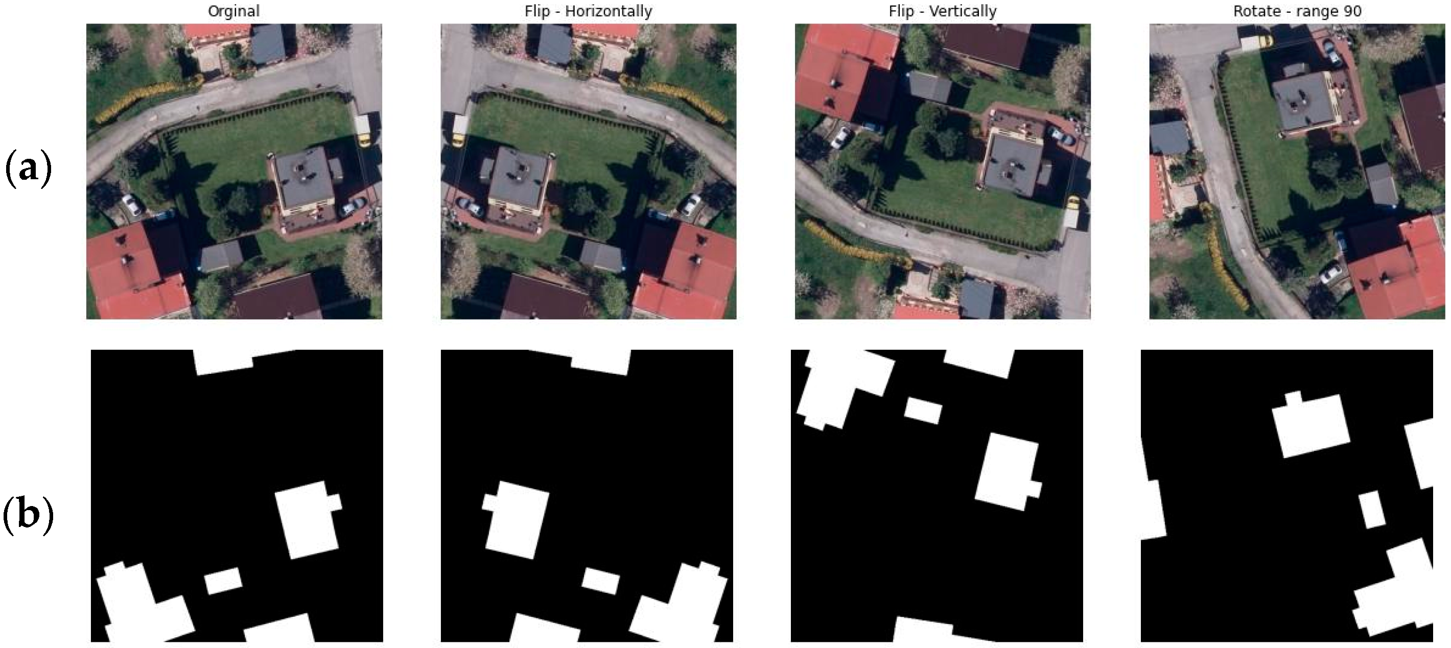
3.2. Data Augmentation

To eliminate overfitting, data augmentation was performed using the ImageDataGenerator class available in the Keras package. The rotation and flip operations were applied to the datasets. The data prepared in this way were used to check whether data augmentation improved the results that were obtained on the validation dataset. Example images that were obtained as a result of data augmentation are presented in Figure 6. The results of network training based on augmented data are presented in Section 4.

3.3. Semantic Image Segmentation

During the development of the computational strategy for the segmentation task, the choice of network hyperparameters was considered and analysed. Special attention was paid to the selection of an appropriate loss function. The most commonly selected loss functions for the segmentation task were described in [46]. Based on the results of the analyses that were presented in the indicated publication, focal loss functions were abandoned. These functions tend to focus on difficult cases of learning patterns. Since images with problems as described in Section 2 could be classified as difficult cases, it was decided not to use this group of loss functions. To confirm the above assumption, the network was also computed using the focal loss function, which proved the above statement.

Finally, a loss function based on the Dice coefficient was chosen, which for binary segmentation is the same as the F1-score metric. This makes it possible to balance between the occurrence of False Positive and False Negative when evaluating the effects of network training. It was therefore considered possible to reduce radial displacement problems in the images in this way. The computational formula of the loss function (1) and (2) is presented below.

$$\mathrm{Dice}\mathrm{coefficient}=\mathrm{F}1\mathrm{score}=\frac{2\times \mathrm{TP}}{2\times \mathrm{TP}+\mathrm{FP}+\mathrm{FN}}\times 100\%$$

(1)

$${\mathrm{L}}_{\mathrm{Dice}}=1-\mathrm{Dice}\mathrm{coefficient}$$

(2)

The Adam optimiser was used for parameter updates [47]. As shown in the analyses conducted by the researchers, it is usually the most efficient [48], also for image segmentation tasks [49]. The optimiser parameters were used according to [47]: learning rate α = 0.001, β1 = 0.9, β2 = 0.999, while ε = 10⁻⁷.

Calculations were carried out on two standalone desktops with GPU computing capability. Computations that used 256 × 256 images were performed on a platform with the parameters: CPU—Intel(R) Core (TM) i7-9750H, GPU—NVIDIA GeForce GTX1650, 16 GB RAM. However, calculations for the second, larger dataset were performed on a platform with the following parameters: CPU—Intel(R) Core (TM) i7-6900K CPU @ 3.20 GHz, GPU—NVIDIA GeForce GTX1070, 62 GB RAM.

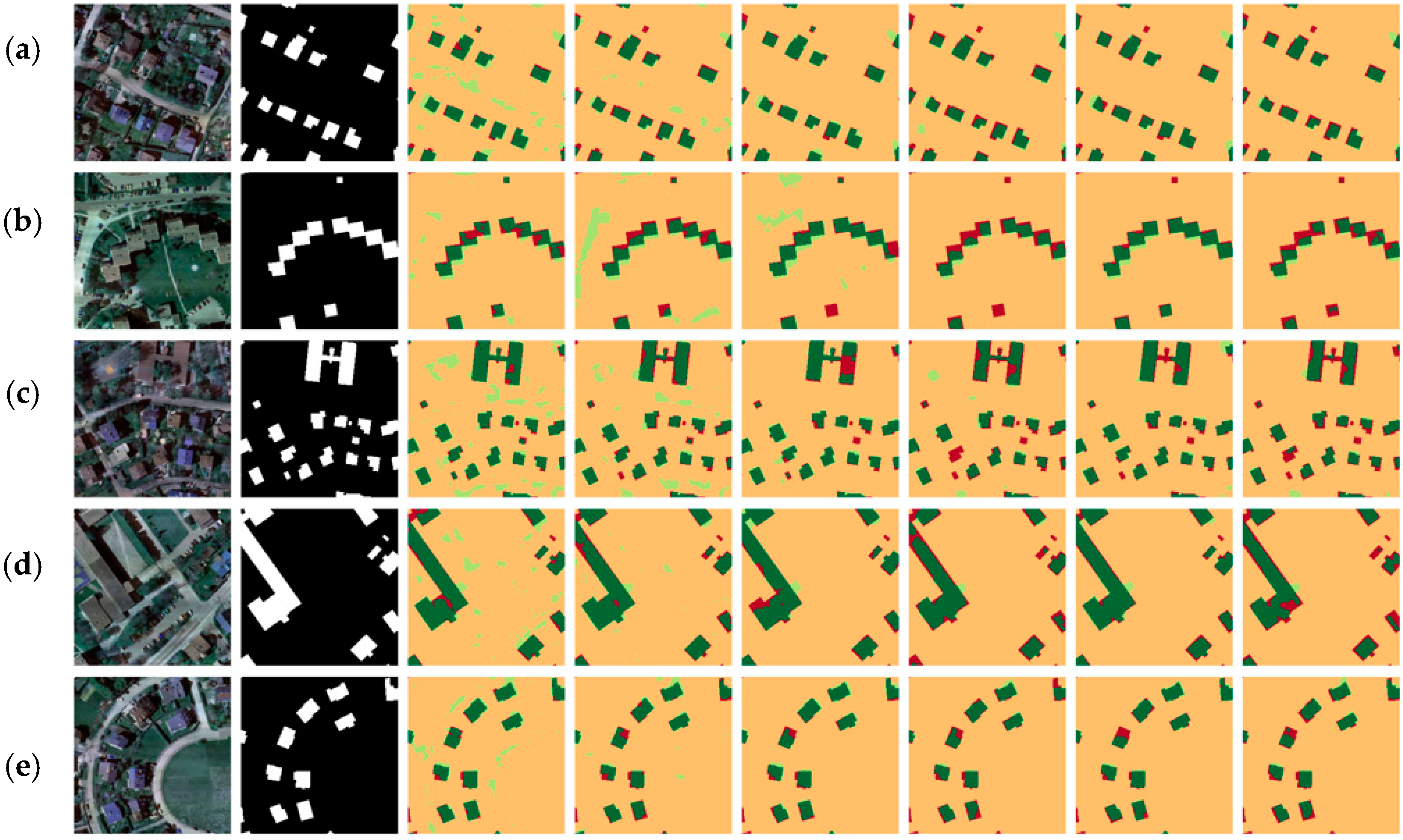
3.4. Results Evaluation

For the network evaluation, the metrics proposed in [50] were used to evaluate the quality of the results obtained in the segmentation task. The following metrics were used: precision (P); recall (R); Intersection-Over-Union (IoU, Jaccard Index); and F1 score (Dice coefficient). These are presented in Equations (3)–(6). The symbols in the formulae indicate elements of the confusion matrix, where: TP—True Positive—number of pixels correctly classified as buildings; FP—False Positive—number of background pixels classified as buildings; TN—True Negative—number of pixels correctly classified as background; and FN—False Negative—number of pixels of buildings classified as background. The average IoU value for both classes—buildings and background—was used in the presentation of the results.

$$\mathrm{precision}=\frac{\mathrm{TP}}{\mathrm{TP}+\mathrm{FP}}$$

(3)

$$\mathrm{recall}=\frac{\mathrm{TP}}{\mathrm{TP}+\mathrm{FN}}$$

(4)

$$\mathrm{IoU}=\frac{\mathrm{TP}}{\mathrm{TP}+\mathrm{FP}+\mathrm{FN}}$$

(5)

$$\mathrm{F}1\mathrm{score}=\frac{2 \times \mathrm{precision} \times \mathrm{recall}}{\mathrm{precision}+\mathrm{recall}}= \frac{2\times \mathrm{TP}}{2\times \mathrm{TP}+\mathrm{FP}+\mathrm{FN}}$$

(6)

4. Results

Before the learning process started, during data loading, all pixels were rescaled to values between 0 and 1. Additionally, the images were normalised. These procedures were intended to speed up the operation of the computational networks. The calculations themselves were performed according to the algorithm described in Section 3. The presented results were obtained on the basis of calculations on a test set. The validation set was used as a control during network learning.

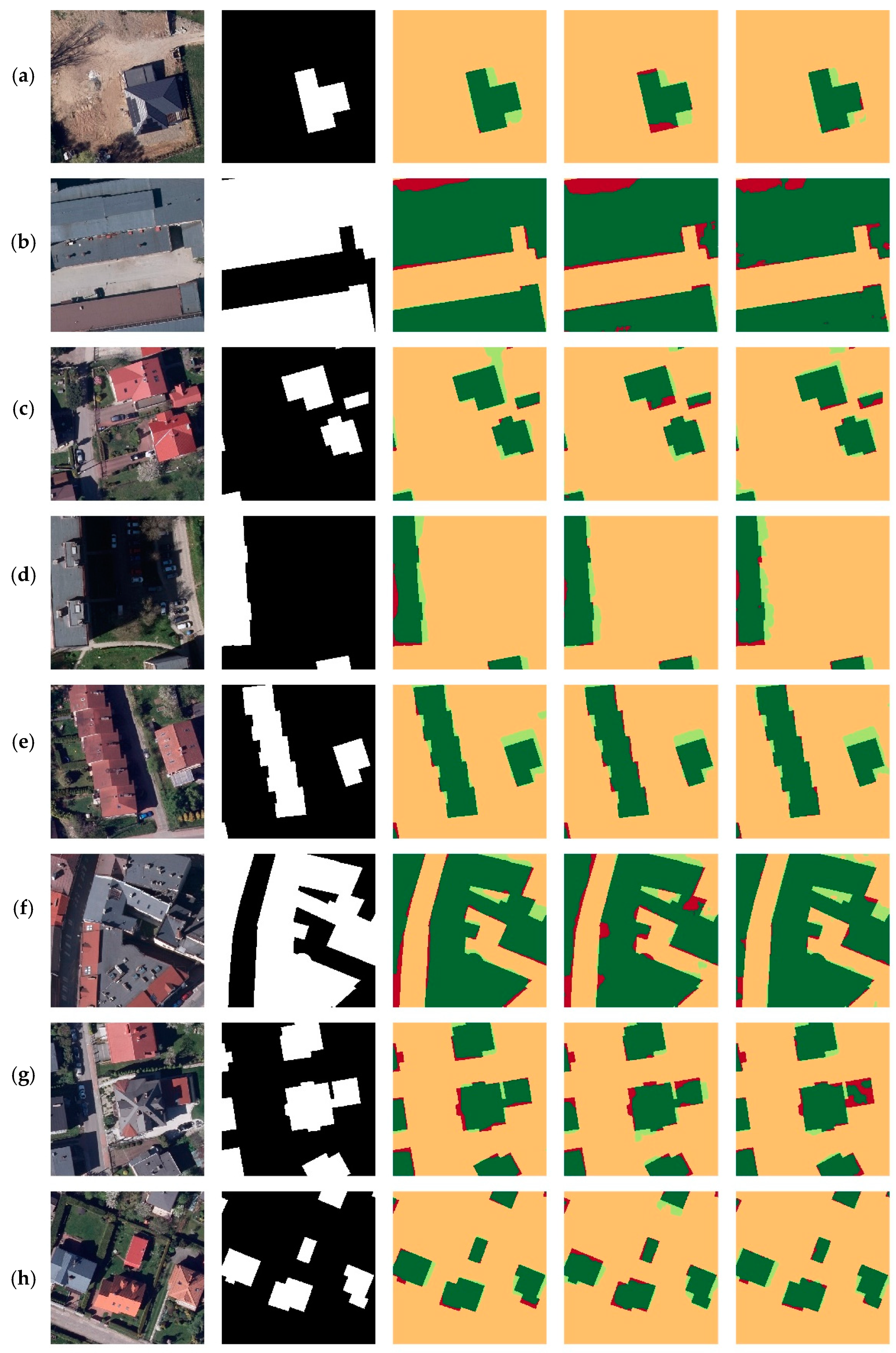
4.1. Dataset with 0.5 m Terrain Pixel

The results that were obtained for a dataset with a 0.5 m pixel are presented in

Table 3. Results for 0.5 m dataset [%].

Neural Network Architecture	Augmentation	mIoU	F1-Score	Precision	Recall
UNET	NO	90.64	95.02	94.89	95.15
UNET with backbone	NO	92.24	95.91	95.83	95.99
DeepLabV3+	NO	79.96	88.37	88.28	88.46
UNET	YES	90.33	94.85	94.57	95.13
UNET with backbone	YES	90.24	94.79	94.53	95.06
DeepLabV3+	YES	83.83	90.81	90.03	91.62

. The best results were achieved for the UNET network with the Resnet34 backbone. In contrast, the worst results were obtained for the DeepLabV3+ network, which may be due to the requirements of this architecture in relation to the number of input datasets. Part of DeepLabV3+ is ASPP (Atrous Spatial Pyramid Pooling) which uses Dilated Convolution. This is computationally demanding [51] and requires sufficient input data of satisfactory quality. The main purpose of using ASPP is to extract features of larger objects and maintain their consistency [7]. Too little input data resulted in False Positive artifacts in some parts of the predicted images. This can be seen in Figure 7, especially in example (c).

Table 3 also shows the results for each architecture using the data augmentation described in Section 3.2. Better results on the test set were obtained only for the DeepLabV3+ architecture, which may confirm the conjecture described in the previous paragraph about the requirements of this network. For both UNET architectures the results achieved are slightly worse. This may be due to the specifics of the dataset and the information transmitted inside the network. As the dataset is characterised by inaccuracies (described in Section 2.2), the network through augmentation may have received more bad patterns for learning. Therefore, the calculated weights changed to recognise more bad patterns. In addition, the data were highly heterogeneous, which results from a lack of spatial planning. It can therefore be concluded that data augmentation does not always produce positive results.

Figure 7 presents the predicted masks based on several images from the test set, which mirrors the results in Table 3. However, not all objects were classified. The reasons for this situation are discussed in detail in Section 4.3.

Ultimately, the UNET architecture with the Resnet34 backbone was found to perform best in terms of both metrics and visualisation. Regular UNET was slightly worse (mIOU worse by 2points). On the other hand, the worst results were obtained for the DeepLabV3+ network—mIOU which was worse than UNET by over 10 points when using the dataset without augmentation and about 7 points when using augmentation.

4.2. Dataset with 0.1 m Terrain Pixel

The results that were obtained by the individual architectures for the dataset with a 0.1 m terrain pixel are presented in

Table 4. Results for 0.1 m dataset [%].

Neural Network Architecture	Augmentation	mIoU	F1-Score	Precision	Recall
UNET	NO	91.08	95.31	95.19	95.43
UNET with backbone	NO	93.00	96.36	96.33	96.38
DeepLabV3+	NO	92.86	96.28	96.27	96.29

. As data augmentation did not significantly improve the results that were achieved for the dataset with a 0.5 m pixel, it was decided to omit it when analysing the dataset with a smaller terrain pixel.

As in the case of the dataset with the 0.5 m terrain pixel, and for the dataset with the 0.1 m terrain pixel, the best performance is achieved by the UNET network with backbone, but the mIoU difference with respect to DeepLabV3+ is small at 0.14 points. This is due to the definition of an appropriate input set size for the DeepLabV3+ network. The regular UNET network performs slightly worse here, the achieved mIoU metric is worse by about 2 points compared to the other networks. However, its biggest advantage is the speed of computation, which is due to the significantly smaller number of weights to be determined.

Visualization of the results is shown in Figure 8. Considering only visual issues, it can be concluded that the best results were obtained for DeepLabV3+ architecture—the most TP and TN areas. The other architectures also give satisfactory results. Importantly, the architectures give good results for both lower density areas (Figure 8a,c–g) and higher density areas (Figure 8b,f).

The occurrence of FP-labelled pixels at the edges of buildings is largely due to the ground truth not being entirely true (errors described in Section 2.2). On the other hand, occurring FNs are often caused by obscuration caused by trees or shading from a taller building. Further, the varied shape of the roof causes the model to fail to recognise parts of the building (TN).

4.3. Discussion

The obtained results confirm the possibility of using open spatial data as a dataset for the task of segmenting buildings from raster images. However, it should be kept in mind that the most important issue is the requirement for data accuracy, which must be adapted to the specific task. Given this, the use of the described approach may have some limitations when the goal is to segment building outlines very accurately, where the problems discussed in Section 2.1 may have a significant impact on the results. This section will discuss the achieved results in more detail.

Firstly, comparing the results that were obtained between the two datasets, one can see slightly higher metric values for the dataset with the smaller ground pixel resolution. This difference is particularly noticeable when using the DeepLabV3+ architecture, where an mIoU score of 12.90 points better was obtained due to the specificity of this architecture. For both UNETs, the difference in value did not exceed 0.01 points, but when visually comparing the results from these networks we see that some of the buildings for the larger pixel were not classified correctly. Such a small difference in metrics is due to the size of the buildings for each dataset. For example, a building with dimensions of 10 × 10 m occupies 20 × 20 pixels for a dataset with a larger pixel and 100 × 100 pixels for a dataset with a smaller pixel. No segmentation of such an object or its shading/shadowing in the test image will have a much greater impact in the case of a dataset with a smaller pixel, and this is reflected during the calculation of metrics.

The visual comparison also shows that the dataset with the smaller terrain pixel is more effective. In the test images, all the objects were correctly identified, whereas the dataset with the larger pixel size showed significantly more False Negative and False Positive areas.

A noticeable problem for both datasets is shaded and wooded areas. Shadows cast by high buildings cause the objects directly below to be covered or shaded. The result is a pixel misclassification or partial segmentation of the object. This problem concerns mainly garages or extensions to the main building. Similar results are generated on images where vegetation—usually trees—covers the image. While the first problem can be eliminated by creating a true-orthophotomap, the second problem in the case of using photogrammetric digital cameras will always occur. Its solution may be the use of LiDAR and adding more analysis dimensions in addition to RGB colours.

The loss function that was used achieved its purpose. The aim of using DICE loss was to maintain a balance between FP and FN values. The results obtained, i.e., similar Recall and Precision values, show that this aim can be considered satisfied.

The mIoU values obtained for building segmentation are similar to those achieved by other researchers for public datasets. Typically, this value reaches a value of around 90%.

The limitations of the used dataset, as described in this section and Section 2.2, may be difficult to fully overcome. The solution of this may be to expand the dataset to include other areas that generate new learning patterns. The analysed dataset was also not varied by lighting, so applying the algorithm to images with different histogram characteristics may not give satisfactory results. Therefore, further tests for more areas, and more diverse areas are possible. In addition, in order to fully assess the accuracy of the obtained results, a comparison of the obtained results with fully correct, hand-made building outlines is required.

The applied models and their hyperparameters can be optimised. However, the aim of this paper was not to develop new architectures or approaches, but to verify the possibility of using open data to generate data for training sets to solve the semantic segmentation problem.

5. Conclusions

Open spatial data allow the extraction of a lot of information. Their biggest advantage is fast and free access. The increase in data volume, combined with the development of machine learning algorithms for object identification increases the ability to accurately extract information from satellite and aerial images. As a result, it is possible to identify the location of objects more accurately at early stages of urban, planning or environmental analyses. It should be remembered, however, that the use of open data depends on the accuracy requirements for the problem being analysed.

On this basis, the analyses presented in this paper conclude that open vector spatial cadastral data can be used as labels in the training process of convolutional neural networks, and solve the task of the semantic segmentation of buildings for raster data. The solution presented in this paper enables simplification of the tedious, time-consuming and capital-intensive process of data labelling. This solution also enables the minimisation of errors that may be reflected in the later results of the analyses. The results of the conducted analyses also allow a comparison of the effectiveness of available popular network architectures, i.e., UNET and DeepLabV3+, in solving semantic segmentation problems, and the influence of backbones on the accuracy of building detection.

This paper also analysed the effect of the orthophoto ground pixel resolution on the accuracy of building identification. The analyses showed that for each of the network architectures used, better results are achieved for data with a smaller terrain pixel. The use of data with a smaller terrain pixel is particularly important when using DeepLabV3+, where it allows the mIoU value to be increased by approximately 13 points.

This needs to be confirmed in separate studies, but most probably these data can be successfully applied for the purposes mentioned in the introduction, such as verifying the state of cadastral databases for the identification of unauthorised buildings; verifying the actual state of the land in the initial phase of the infrastructural investment process for a more reliable cost assessment; the mapping of buildings for unmapped areas; verifying the validity of open databases.

However, it is important to keep in mind the identified limitations of the datasets described in Section 2, such as the building outline following the walls rather than the roof or radial offsets. These limitations were omitted in this analysis as unimportant to the problem being solved. However, they may reduce the efficiency of directly implementing the presented algorithm to solve other problems, such as the accurate detection of the position of buildings.

Therefore, the authors plan to further develop the presented dataset with other, more diverse areas, which will allow to generate new learning patterns and optimise the hyperparameters of the applied models in order to increase the accuracy of object detection.

The authors also plan to apply the algorithm presented in this paper using true-orthophoto mapping, which should become more widely available for a larger area of Poland over time. This approach will allow examination of the extent to which the reduction in radial displacement problems improves the extraction of buildings using the algorithm presented in this paper. Additionally, in order to minimise the problem of detecting objects under vegetation and shaded areas, the possibility of adding more image dimensions on the basis of available LiDAR data from Airborne Laser Scanning also made available by governmental units will be verified.

Moreover, the authors are planning to compare a dataset for which masks will be created manually with a dataset that includes masks adopted based on cadastral data. The aim of this activity will be to verify the existence of the algorithm limitations that are proposed in this publication.

References

1. European Commission. Open Data Maturity Report 2020; European Commission: Brussels, Belgium, 2020. [Google Scholar]
2. Liu, P.; Liu, X.; Liu, M.; Shi, Q.; Yang, J.; Xu, X.; Zhang, Y. Building footprint extraction from high-resolution images via spatial residual inception convolutional neural network. Remote Sens. 2019, 11, 830. [Google Scholar] [CrossRef] [Green Version]
3. Touzani, S.; Granderson, J. Open data and deep semantic segmentation for automated extraction of building footprints. Remote Sens. 2021, 13, 2578. [Google Scholar] [CrossRef]
4. Liu, J.; Wang, S.; Hou, X.; Song, W. A deep residual learning serial segmentation network for extracting buildings from remote sensing imagery. Int. J. Remote Sens. 2020, 41, 5573–5587. [Google Scholar] [CrossRef]
5. Li, W.; He, C.; Fang, J.; Fu, H. Semantic segmentation based building extraction method using multi-source GIS map datasets and satellite imagery. In Proceedings of the 2018 IEEE/CVF Conference on Computer Vision and Pattern Recognition Workshops (CVPRW), Salt Lake City, UT, USA, 18–22 June 2018; pp. 233–236. [Google Scholar] [CrossRef]
6. Chen, Z.; Li, D.; Fan, W.; Guan, H.; Wang, C.; Li, J. Self-attention in reconstruction bias U-net for semantic segmentation of building rooftops in optical remote sensing images. Remote Sens. 2021, 13, 2524. [Google Scholar] [CrossRef]
7. Wang, H.; Miao, F. Building extraction from remote sensing images using deep residual U-Net. Eur. J. Remote Sens. 2022, 55, 71–85. [Google Scholar] [CrossRef]
8. Bischke, B.; Helber, P.; Folz, J.; Borth, D.; Dengel, A. Multi-Task Learning for Segmentation of Building Footprints with Deep Neural Networks. In Proceedings of the 2019 IEEE International Conference on Image Processing (ICIP), Taipei, Taiwan, 22–25 September 2019; pp. 1480–1484. [Google Scholar] [CrossRef] [Green Version]
9. Yi, Y.; Zhang, Z.; Zhang, W.; Zhang, C.; Li, W.; Zhao, T. Semantic segmentation of urban buildings from VHR remote sensing imagery using a deep convolutional neural network. Remote Sens. 2019, 11, 1774. [Google Scholar] [CrossRef] [Green Version]
10. He, H.; Yang, D.; Wang, S.; Wang, S.; Li, Y. Road extraction by using atrous spatial pyramid pooling integrated encoder-decoder network and structural similarity loss. Remote Sens. 2019, 11, 1015. [Google Scholar] [CrossRef] [Green Version]
11. Boonpook, W.; Tan, Y.; Bai, B.; Xu, B. Road Extraction from UAV Images Using a Deep ResDCLnet Architecture. Can. J. Remote Sens. 2021, 47, 450–464. [Google Scholar] [CrossRef]
12. Gupta, A.; Watson, S.; Yin, H. Deep learning-based aerial image segmentation with open data for disaster impact assessment. Neurocomputing 2021, 439, 22–33. [Google Scholar] [CrossRef]
13. Robinson, C.; Hohman, F.; Dilkina, B. A deep learning approach for population estimation from satellite imagery. In Proceedings of the 1st ACM SIGSPATIAL Workshop on Geospatial Humanities, Online, 7 November 2017; pp. 47–54. [Google Scholar] [CrossRef] [Green Version]
14. Cai, L.; Xu, X.; Liew, J.H.; Sheng Foo, C. Revisiting Superpixels for Active Learning in Semantic Segmentation with Realistic Annotation Costs. In Proceedings of the 2021 IEEE/CVF Conference on Computer Vision and Pattern Recognition (CVPR), Nashville, TN, USA, 20–25 June 2021; pp. 10983–10992. [Google Scholar] [CrossRef]
15. Li, Y.; Chen, J.; Xie, X.; Ma, K.; Zheng, Y. Self-loop uncertainty: A novel pseudo-label for semi-supervised medical image segmentation. In Medical Image Computing and Computer Assisted Intervention—MICCAI 2020; Lecture Notes in Computer Science (Including Subseries Lecture Notes in Artificial Intelligence and Lecture Notes in Bioinformatics); Springer: Cham, Switzerland, 2020; Volume 12621, pp. 614–623. [Google Scholar] [CrossRef]
16. Sun, W.; Zhang, J.; Barnes, N. 3D Guided Weakly Supervised Semantic Segmentation. In Computer Vision—ACCV 2020; Lecture Notes in Computer Science (Including Subseries Lecture Notes in Artificial Intelligence and Lecture Notes in Bioinformatics); Springer: Cham, Switzerland, 2020; Volume 12622, pp. 585–602. [Google Scholar] [CrossRef]
17. Maggiori, E.; Tarabalka, Y.; Charpiat, G.; Alliez, P. Can semantic labeling methods generalize to any city? the inria aerial image labeling benchmark. In Proceedings of the 2017 IEEE International Geoscience and Remote Sensing Symposium (IGARSS), Fort Worth, TX, USA, 23–28 July 2017; pp. 3226–3229. [Google Scholar] [CrossRef] [Green Version]
18. Farasin, A.; Colomba, L.; Garza, P. Double-step U-Net: A deep learning-based approach for the estimation ofwildfire damage severity through sentinel-2 satellite data. Appl. Sci. 2020, 10, 4332. [Google Scholar] [CrossRef]
19. Ulmas, P.; Liiv, I. Segmentation of Satellite Imagery using U-Net Models for Land Cover Classification. arXiv 2020, arXiv:2003.02899. [Google Scholar]
20. Gargiulo, M.; Dell’aglio, D.A.G.; Iodice, A.; Riccio, D.; Ruello, G. Integration of sentinel-1 and sentinel-2 data for land cover mapping using w-net. Sensors 2020, 20, 2969. [Google Scholar] [CrossRef] [PubMed]
21. Karra, K.; Kontgis, C.; Statman-Weil, Z.; Mazzariello, J.C.; Mathis, M.; Brumby, S.P. Global Land Use/Land Cover with Sentinel 2 and Deep Learning. In Proceedings of the 2021 IEEE International Geoscience and Remote Sensing Symposium IGARSS, Brussels, Belgium, 11–16 July 2021; pp. 4704–4707. [Google Scholar] [CrossRef]
22. Pan, Z.; Xu, J.; Guo, Y.; Hu, Y.; Wang, G. Deep learning segmentation and classification for urban village using a worldview satellite image based on U-net. Remote Sens. 2020, 12, 1574. [Google Scholar] [CrossRef]
23. Shahi, K.; Shafri, H.Z.M.; Taherzadeh, E.; Mansor, S.; Muniandy, R. A novel spectral index to automatically extract road networks from WorldView-2 satellite imagery. Egypt. J. Remote Sens. Sp. Sci. 2015, 18, 27–33. [Google Scholar] [CrossRef] [Green Version]
24. Boguszewski, A.; Batorski, D.; Ziemba-Jankowska, N.; Dziedzic, T.; Zambrzycka, A. LandCover.ai: Dataset for automatic mapping of buildings, woodlands, water and roads from aerial imagery. In Proceedings of the IEEE Computer Society Conference on Computer Vision and Pattern Recognition Workshops, Nashville, TN, USA, 19–25 June 2021; pp. 1102–1110. [Google Scholar]
25. Directive 2007/2/EC of the European Parliament and of the Council of 14 March 2007 Establishing an Infrastructure for Spatial Information in the European Community (INSPIRE). Available online: https://eur-lex.europa.eu/legal-content/EN/ALL/?uri=CELEX%3A32007L0002 (accessed on 15 March 2022).
26. Geoportal Krajowy (National Geoportal). Available online: https://www.geoportal.gov.pl/ (accessed on 15 March 2022).
27. Ewidencja Zbiorów i Usług Danych Przestrzennych (Register of Spatial Data Sets and Services). Available online: https://integracja.gugik.gov.pl/eziudp/ (accessed on 15 March 2022).
28. Habib, A.F.; Kim, E.M.; Kim, C.J. New methodologies for true orthophoto generation. Photogramm. Eng. Remote Sens. 2007, 73, 25–36. [Google Scholar] [CrossRef] [Green Version]
29. Glinka, S. Keras Segmentation Models. Available online: https://github.com/sajmonogy/keras_segmentation_models (accessed on 1 May 2022).
30. Badrinarayanan, V.; Kendall, A.; Cipolla, R. SegNet: A Deep Convolutional Encoder-Decoder Architecture for Image Segmentation. IEEE Trans. Pattern Anal. Mach. Intell. 2017, 39, 2481–2495. [Google Scholar] [CrossRef]
31. Abdollahi, A.; Pradhan, B.; Alamri, A.M. An ensemble architecture of deep convolutional Segnet and Unet networks for building semantic segmentation from high-resolution aerial images. Geocarto Int. 2020, 35, 1856199. [Google Scholar] [CrossRef]
32. Zhao, H.; Shi, J.; Qi, X.; Wang, X.; Jia, J. Pyramid scene parsing network. In Proceedings of the 2017 IEEE Conference on Computer Vision and Pattern Recognition (CVPR), Honolulu, HI, USA, 21–26 July 2017; pp. 6230–6239. [Google Scholar] [CrossRef] [Green Version]
33. Weng, W.; Zhu, X. UNet: Convolutional Networks for Biomedical Image Segmentation. IEEE Access 2021, 9, 16591–16603. [Google Scholar] [CrossRef]
34. Li, R.; Liu, W.; Yang, L.; Sun, S.; Hu, W.; Zhang, F.; Li, W. DeepUNet: A Deep Fully Convolutional Network for Pixel-Level Sea-Land Segmentation. IEEE J. Sel. Top. Appl. Earth Obs. Remote Sens. 2018, 11, 3954–3962. [Google Scholar] [CrossRef] [Green Version]
35. Sofla, R.A.D.; Alipour-Fard, T.; Arefi, H. Road extraction from satellite and aerial image using SE-Unet. J. Appl. Remote Sens. 2021, 15, 014512. [Google Scholar] [CrossRef]
36. He, N.; Fang, L.; Plaza, A. Hybrid first and second order attention Unet for building segmentation in remote sensing images. Sci. China Inf. Sci. 2020, 63, 140305. [Google Scholar] [CrossRef] [Green Version]
37. Chen, L.C.; Papandreou, G.; Kokkinos, I.; Murphy, K.; Yuille, A.L. Semantic Image Segmentation with Deep Convolutional Nets and Fully Connected CRFs. arXiv 2015, arXiv:1412.7062. [Google Scholar]
38. Chen, L.C.; Papandreou, G.; Kokkinos, I.; Murphy, K.; Yuille, A.L. DeepLab: Semantic Image Segmentation with Deep Convolutional Nets, Atrous Convolution, and Fully Connected CRFs. IEEE Trans. Pattern Anal. Mach. Intell. 2018, 40, 834–848. [Google Scholar] [CrossRef] [PubMed] [Green Version]
39. Chen, L.-C.; Papandreou, G.; Schroff, F.; Adam, H. Rethinking Atrous Convolution for Semantic Image Segmentation. arXiv 2017, arXiv:1706.05587. [Google Scholar]
40. Chen, L.C.; Zhu, Y.; Papandreou, G.; Schroff, F.; Adam, H. Encoder-decoder with atrous separable convolution for semantic image segmentation. In Computer Vision—ECCV 2018; Lecture Notes in Computer Science (Including Subseries Lecture Notes in Artificial Intelligence and Lecture Notes in Bioinformatics); Springer: Cham, Switzerland, 2018; Volume 11211, pp. 833–851. [Google Scholar] [CrossRef] [Green Version]
41. Liu, C.; Chen, L.C.; Schroff, F.; Adam, H.; Hua, W.; Yuille, A.L.; Fei-Fei, L. Auto-deeplab: Hierarchical neural architecture search for semantic image segmentation. In Proceedings of the 2019 IEEE/CVF Conference on Computer Vision and Pattern Recognition (CVPR), Long Beach, CA, USA, 15–20 June 2019; pp. 82–92. [Google Scholar] [CrossRef] [Green Version]
42. Liu, Z.; Liu, W.; Qi, H.; Li, Y.; Zhang, G.; Zhang, T. Extracting River Illegal Buildings from UAV Image Based on Deeplabv3+. In Geoinformatics in Sustainable Ecosystem and Society, Proceedings of the 7th International Conference, GSES 2019, and First International Conference, GeoAI 2019, Guangzhou, China, 21–25 November 2019; Springer: Singapore, 2020; Volume 1228, pp. 259–272. [Google Scholar] [CrossRef]
43. Xiang, S.; Xie, Q.; Wang, M. Semantic Segmentation for Remote Sensing Images Based on Adaptive Feature Selection Network. In IEEE Geoscience and Remote Sensing Letters; IEEE: New York, NY, USA, 2022; Volume 19. [Google Scholar] [CrossRef]
44. Zhang, D.; Ding, Y.; Chen, P.; Zhang, X.; Pan, Z.; Liang, D. Automatic extraction of wheat lodging area based on transfer learning method and deeplabv3+ network. Comput. Electron. Agric. 2020, 179, 105845. [Google Scholar] [CrossRef]
45. Yakubovskiy, P. Segmentation Models. Available online: https://github.com/qubvel/segmentation_models (accessed on 5 March 2022).
46. Jadon, S. A survey of loss functions for semantic segmentation. In Proceedings of the 2020 IEEE Conference on Computational Intelligence in Bioinformatics and Computational Biology (CIBCB), Via del Mar, Chile, 27–29 October 2020. [Google Scholar] [CrossRef]
47. Kingma, D.P.; Ba, J.L. Adam: A method for stochastic optimization. In Proceedings of the 3rd International Conference for Learning Representations, San Diego, CA, USA, 7–9 May 2015; pp. 1–15. [Google Scholar]
48. Schneider, F.; Balles, L.; Hennig, P. Deepobs: A deep learning optimizer benchmark suite. In Proceedings of the 7th International Conference on Learning Representations, ICLR 2019, New Orleans, LA, USA, 6–9 May 2019; pp. 1–14. [Google Scholar]
49. Yaqub, M.; Jinchao, F.; Zia, M.S.; Arshid, K.; Jia, K.; Rehman, Z.U.; Mehmood, A. State-of-the-art CNN optimizer for brain tumor segmentation in magnetic resonance images. Brain Sci. 2020, 10, 427. [Google Scholar] [CrossRef]
50. Minaee, S.; Boykov, Y.Y.; Porikli, F.; Plaza, A.J.; Kehtarnavaz, N.; Terzopoulos, D. Image Segmentation Using Deep Learning: A Survey. IEEE Trans. Pattern Anal. Mach. Intell. 2021, 14, 3523–3542. [Google Scholar] [CrossRef]
51. Wang, Z.; Ji, S. Smoothed dilated convolutions for improved dense prediction. In Proceedings of the 24th ACM SIGKDD International Conference on Knowledge Discovery & Data Mining, KDD 2018, London, UK, 19–23 August 2018; pp. 2486–2495. [Google Scholar] [CrossRef] [Green Version]
Figure 1. Comparison of data from EGIB and OSM (green—common parts of both databases, yellow—objects only in EGiB database, red—objects only in OSM database).
Remotesensing 14 02745 g001
Figure 2. Identified errors for input data. Red colour marks outlines of buildings from the cadastral database. The images represent, respectively, the problems: (a) outline along the building walls—not along the roof, (b) gaps in the EGiB database, (c) radial displacement for tall buildings, (d) correct outline.
Remotesensing 14 02745 g002aRemotesensing 14 02745 g002b
Figure 3. Algorithm for preparing datasets.
Remotesensing 14 02745 g003
Figure 4. Comparison of datasets: (a) with 0.1 m pixel, (b) with 0.5 m pixel.
Remotesensing 14 02745 g004
Figure 5. Used model architectures.
Remotesensing 14 02745 g005
Figure 6. Example of augmented data: (a) images (b) masks.
Remotesensing 14 02745 g006
Figure 7. Visualisation of the results for the 0.5 m dataset. From left: input image, ground truth, DeepLab, DeepLab with augmentation, UNET, UNET with augmentation, UNET_bb, UNET_bb with augmentation. Colours: dark green—TP, orange—TN, light green—FP, red—FN. (ae) various examples from the test dataset.
Remotesensing 14 02745 g007
Figure 8. Visualisation of the results for the 0.1 m dataset. From left: input image, ground truth, DeepLabV3+, UNET, UNET with backbone. Colours: dark green—TP, orange—TN, light green—FP, red—FN. (ah) various examples from the test dataset.
Remotesensing 14 02745 g008