Calibration of Co-Located Identical PAR Sensors Using Wireless Sensor Networks and Characterization of the In Situ fPAR Variability in a Tropical Dry Forest

Abstract

The fraction of photosynthetic active radiation (fPAR) attempts to quantify the amount of enery that is absorbed by vegetation for use in photosynthesis. Despite the importance of fPAR, there has been little research into how fPAR may change with biome and latitude, or the extent and number of ground networks required to validate satellite products. This study provides the first attempt to quantify the variability and uncertainties related to in-situ 2-flux fPAR estimation within a tropical dry forest (TDF) via co-located sensors. Using the wireless sensor network (WSN) at the Santa Rosa National Park Environmental Monitoring Super Site (Guanacaste, Costa Rica), this study analyzes the 2-flux fPAR response to seasonal, environmental, and meteorological influences over a period of five years (2013–2017). Using statistical tests on the distribution of fPAR measurements throughout the days and seasons based on the sky condition, solar zenith angle, and wind-speed, we determine which conditions reduce variability, and their relative impact on in-situ fPAR estimation. Additionally, using a generalized linear mixed effects model, we determine the relative impact of the factors above, as well as soil moisture on the prediction of fPAR. Our findings suggest that broadleaf deciduous forests, diffuse light conditions, and low wind patterns reduce variability in fPAR, whereas higher winds and direct sunlight increase variability between co-located sensors. The co-located sensors used in this study were found to agree within uncertanties; however, this uncertainty is dominated by the sensor drift term, requiring routine recalibration of the sensor to remain within a defined criteria. We found that for the Apogee SQ-110 sensor using the manufacturer calibration, recalibration around every 4 years is needed to ensure that it remains within the 10% global climate observation system (GCOS) requirement. We finally also find that soil moisture is a significant predictor of the distribution and magnitude of fPAR, and particularly impacts the onset of senescence for TDFs.

1. Introduction

A prominent field in remote sensing is monitoring forest productivity and how it changes over time in response to disturbances and climate change [1]. Forest productivity or net primary productivity (NPP) is linearly related to the photosynthetic active radiation (PAR) via the actual light use efficiency coefficient, so NPP_(x,t) = APAR_(x,t) − ε_(x,t). Where APAR_(x,t) is the absorbed PAR by pixel x at time t (e.g., month), and ε_(x,t) represents the actual light use efficiency at pixel x at time t. Since 1996, and as a result of the development of new sensing techniques and instruments, the fraction of PAR or fPAR has been defined in many different ways; however, it is consistently considered a biophysical variable that can be used for quantifying the amount of PAR (PAR; 400–700 nm) absorbed for photosynthesis by vegetation [2,3,4,5,6,7,8,9,10]. The research into fPAR has resulted in it being considered an essential variable for monitoring forest and ecosystem health and productivity. This variable has also been used extensively for estimating production efficiency models (PEMs) and NPP [11,12,13,14,15], and it has further been declared an essential climate variable (ECV) by both the global climate observation system (GCOS) and global terrestrial observation system (GTOS).

As the suite of land satellite products has increased, there has also been an increased need for these products to undergo a validation process [16]. The fPAR can be derived from both satellite data, such as NASA’s moderate resolution imaging spectroradiometer (MODIS) satellite systems [5] and from in-situ measurements. The fPAR can be determined at a local level both through direct measurements [10,17,18,19,20,21] and through derivation from radiative transfer models [8,22,23].

Direct methods for estimating fPAR usually result in large, costly, and technical experimental field setups [7,20,21,24,25] while indirect methods, in general, use the gap fractions retrieved from hemispherical photographs [26], which relate to leaf area and allow for fPAR derivation [27,28]. More recently, modeling approaches have become common due to financial and time constraints [4,6,14,29,30]. These studies have acknowledged the complexity of light environments, especially in forest ecosystems that exhibit a high degree of spatial heterogeneity [8,31,32,33]; however, these experimental methods are dependent on radiation measurements from a few sensors and neglect the hetrogeneity of the light fields they are measuring [18].

Scientific bodies, such as the Committee on Earth Observation Satellites—Land Product Validation (EOS-LPV) sub-group have, therefore, called for the expansion and diversification of in-situ calibration and validation sites to provide a robust and globally representative quality-assured product [16]. Additionally, these scientific bodies have also called for the establishment of standardized protocols for the measurement and reporting of uncertainties for in-situ fPAR products. This standardization and expansion of sites will improve satellite-derived fPAR validation, and ensure higher quality products, as outlined by the CEOS-LPV validation hierarchy [16]. To date, there have been no sites used to quantify the uncertainty of fPAR using this standardized approach in the tropical dry forest, a biome that accounts for 40% of tropical ecosystems [34]. Given the extensive nature of this biome, and its highly heterogeneous structure, quantifying and validating fPAR in this biome is crucial.

Due to the increasing need for standardization in validation methodologies, this study uses the definitions and methodologies originally put forward in Widlowski [10] and furthered by Nestola et al. [20] and Putzenlechner et al. [24]. Widlowski compared a variety of fPAR measurements and determined that the 2-flux fPAR measurement was the most invariant in-situ fPAR flux. Both Nestola et al. [20] and Putzenlechner et al. [24] expanded the scale of the experiments, both temporally and spatially. They further illustrated how a wireless sensor network (WSN) composed of data loggers (or nodes) and equipped with environmental sensors capable of sampling and storing understory micrometeorological data can be utilized in the analysis of fPAR [20,24]. The use of a network of data loggers in the understory of heterogeneous forests, permits the uncertainty and variability to be quantified over daily to multiyear timeframes [35,36,37,38].

Based on these considerations and gaps in knowledge, we employ a WSN in the tropical dry forest in Santa Rosa National Park (Costa Rica) Environmental Monitoring Super Site, to determine the 2-flux fPAR. We investigate the spatial, temporal, and environmental factors that cause variability in the in-situ 2-flux fPAR product within a TDF, with a focus on the impact of the solar zenith angle, sky conditions, and wind speed. Data from pairs of co-located sensors are used to address uncertainties and recalibration needs in order to create a robust in-situ 2-flux fPAR product that can meet the standards outlined by the GCOS [39].

2. Materials and Methods

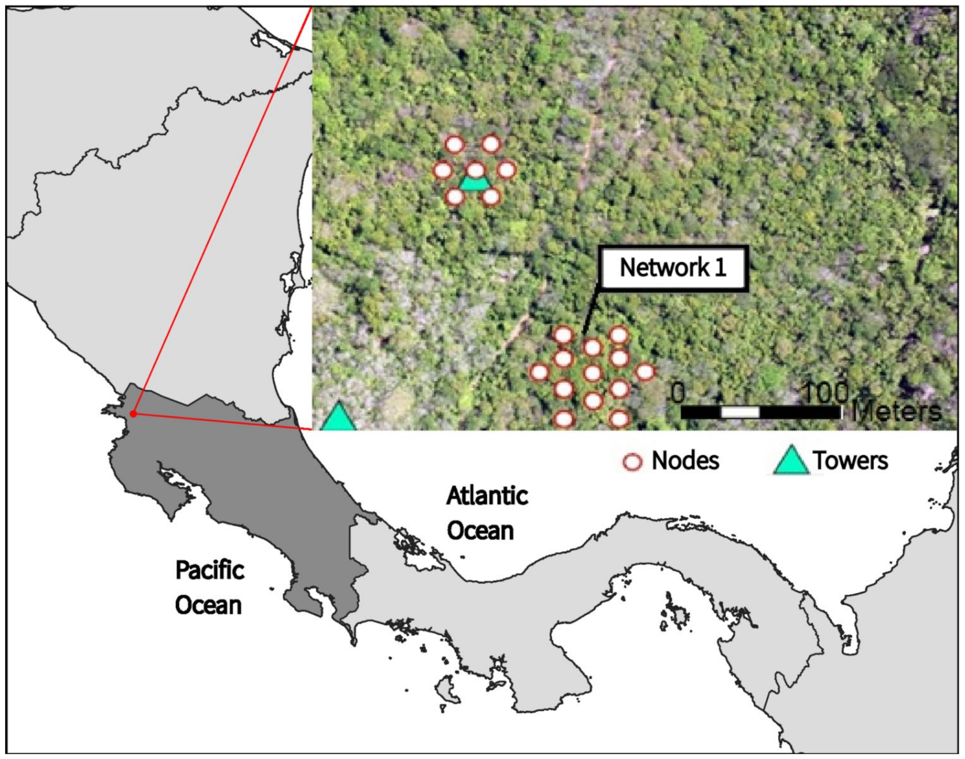
2.1. Study Site

This study was conducted at the Santa Rosa National Park Environmental Monitoring Super Site (SRNP-EMSS) located in Guanacaste, Costa Rica (Figure 1). Santa Rosa is considered a transitional tropical dry forest to tropical moist forest, with the uplands including a matrix of secondary tropical dry forest (TDF) of various ages and varied histories of anthropogenic land use [40,41,42]. There is between 900–2500mm of rainfall per year, falling in a wet–dry seasonal cycle, and an average temperature of ≥25 °C [43].

Of the two WSN networks present in this specific area of the super site, only one was used in this study (Figure 1 and Figure 2). The selected WSN covers an area of 75 × 65 m (4875 m²) and contains 48 subplots that measure 10 × 10 m (100m²). The WSN has a total of 13 nodes (small wireless data loggers with four digital and analog outputs). Five nodes have installed two co-located PAR sensors (black squares in Figure 2), and eight nodes have just one PAR sensor (open circles in Figure 2). The area monitored by the selected WSN has 39 different tree species, with an average diameter at breast height (DBH) of 0.131 m, and an estimated average tree height of 9 m. The basal area per subplot within the WSN ranges from 124.6 m² ha⁻¹ to 714.2 m² ha⁻¹. Of the 39 species found within the footprint of the WSN, Guazuma ulmifolia, Luehea speciosa, and Lueahea candida accounted for 18%, 11%, and 8% of the total stems. All tree species found within the WSN were classified as deciduous broadleaf trees, exhibiting seasonal leaf loss during the dry season or senescence period.

2.2. Instrumentation

For this study, the WSN with the longest and most complete record was chosen, and data from 2013–2017 were compiled. In the network, there are 13 self-powered nodes (model ENV-Link-Mini-LXRS, Lord Microstrain, Cary, NC, USA). Each node is equipped with a temperature and relative humidity sensor, along with soil moisture and quantum PAR sensors (model SQ-110, Apogee, Logan, UT, USA., field of view 180°) located 1.3m from the forest floor. The PAR sensors measure PAR that is transmitted (tPAR µE) from the atmosphere through the canopy and into the understory. These PAR sensors have manufacturer-determined uncertainty estimates as follows: cosine response +/−5% at 75° solar zenith angle (SZA), temperature response 0.06 +/− 0.06% per °C, calibration uncertainty +/−5%, and non-stability <2% per year. This information provides a building block to developing a quality control process for PAR monitoring.

The distribution of nodes within the network was chosen based on installation >80 m from the edge of the forest to avoid edge effects and a domain of interest greater than 30 m × 30 m [10] to reduce bias due to horizontal fluxes. A star-like arrangement of nodes within the network was chosen to: (a) maximize the area covered by the nodes, (b) prevent the formation of gaps between sensors resulting in the incomplete characterization of the overhead canopy, and (c) guarantee wireless sensor connectivity across the network (Figure 2) [24,38,44,45]. These formations have also been found to be less influenced by solar zenith angle (SZA) compared to other distributions, such as transect alignments [10].

Additionally, there is a single companion meteorological tower located within 200 m of all nodes in the network (Figure 2). This tower has SQ-110 quantum PAR sensors mounted at 36 m from the ground, which measure incoming PAR (iPAR) from the atmosphere, and total reflected PAR (rPAR) coming from the soil, leaf litter, and canopy. There is also an onset hobo datalogger, which measures wind speed, gust speed, wind direction, air temperature, relative humidity, barometric pressure, incoming net radiation, and reflected net radiation on the tower. Sampling is set at a 2-s interval and aggregated to a 30-min mean value. These observations are wirelessly transmitted to enviro-net.org©. Enviro-Net is a comprehensive data repository that allows uploading, retrieval and analysis of information collected using WSNs. Access to the data repository is free.

2.3. Calibration of PAR Sensors

Sensor calibration and drift monitoring are crucial components of a long-term environmental monitoring program. These two components are necessary if the calibration and validation community will use information collected from WSNs to support calibration and validation activities of current and future remote-sensing missions. Proper follow-up on sensor drift can provide important information about long-term data quality as part of quality control processes. In addition, from a management perspective, calibration and sensor drift offers essential insights into the need for sensor replacement, so the data collected are within the manufacturer’s specifications.

Within the longer deployment at the SRNP-EMSS, a nominally 13-month experiment was conducted, where five pairs of co-located sensors were deployed to address variability and calibration aspects. Records run from April 2015 to November 2015 (Node 1) as a minimum = 8 months, to April 2015 to April 2016 (Node 4) = 13 months. The five paired sensors were identical SQ-110 PAR units, with one sensor solely reliant on the manufacturer calibration, and the second sensor independently calibrated at the National Physical Laboratory (NPL, Teddington, UK). Figure 2 provides a spatial context for the locations of the nodes and sensors used in this study.

The Apogee (manufacturer) calibration uses a comparison to the LiCOR 1800-02 Optical Radiation Calibrator [46,47]. The manufacturer compares a suite of SQ-110 sensors against several references to derive a general calibration coefficient and uncertainty, which is applied to all SQ-100 range sensors [46]. This batch processing may lead to larger uncertainties, including spectral errors as the SQ-110 responds differently compared to the reference sensor under different sky conditions. However, all these effects are characterized in the manufacturer quoted uncertainties.

The NPL calibration approach updated the sensor calibration coefficients. The sensor spectral response was independently measured and calibrated via a known spectral broadband irradiance source with the uncertainty calculated according to the guide to the expression of uncertainty in measurement [48]. Correction factors for typical illumination spectra were generated (e.g., diffuse sky and vegetation) and applied to the measured data. The quoted calibration accuracy does not include any consideration for the field operational illumination conditions.

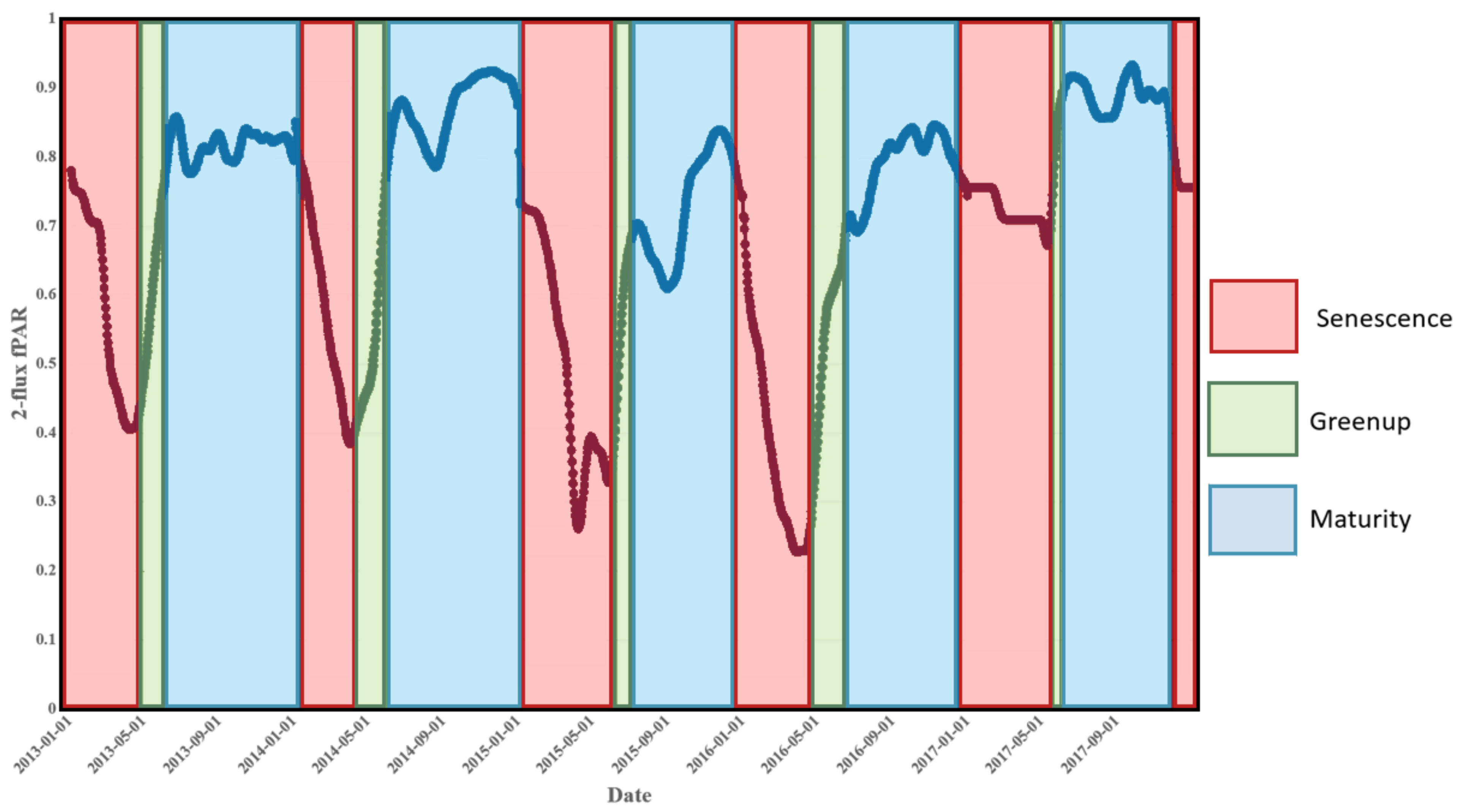
2.4. Data Processing

In processing the fPAR data, timesteps where tPAR > iPAR were excluded, as they were theorized to be caused by clouds passing overhead the iPAR sensors but not the tPAR sensors. SZA and air temperature corrections were applied to the PAR values. These corrections can adjust values by up to 0.06 +/− 0.06% per °C away from 20 °C and by +/−5% for SZA > 75°.

The 2-flux fPAR was then calculated using:

$$1-\mathrm{flux} \mathrm{fPAR}=1-\frac{\mathrm{tPAR}}{\mathrm{iPAR}}$$

(1)

where tPAR is the transmitted PAR in the understory, and iPAR is the incident PAR from the tower. This formula is considered robust especially for in-situ and WSN analyses [10,24]. This flux was calculated every 10 min during daylight hours for every node. The nodes were synchronized using timestamps and could then be averaged to create a single network-wide 2-flux fPAR (2-flux fPAR_Domain).

The fPAR was also categorized by sky conditions, which were classified as clear (CS), mixed (MS), and diffuse (DS) based on the clear-sky calculator developed by Walter [49]. Sky conditions (measured at the top of the meteorological tower (h = 36 m) are determined to be diffuse when iPAR < 900 µE, mixed when 900 µE < iPAR < 1100 µE, and clear when iPAR > 1100 µE. This characterization was necessary due to the absence of sunshine pyranometers. These sensors allow for the determination of diffuse-to-total incident radiation, a metric used by other studies [6,10,24].

The 2-flux fPAR data were also categorized into three phenophases to isolate the environmental conditions that drive extreme changes in 2-flux fPAR (2-flux fPAR = 0.01 – 0.99). The three phenophases (green-up, maturity, and senescence) were determined using slope threshold values between the minimum and maximum 2-flux fPAR values ([50]; Figure 3). The time-series (2013–2017) was divided into the three phenophases for each growing season resulting in six senescence (n = 4548), five green-up (n = 1331), and five maturity (n = 9711) phases in total (Figure 3).

The regression analysis for the co-located sensors involves the estimation of two different types of curve fitting. The type ft0 corresponds to a forced zero intercept linear regression, and ft1 corresponds to an unrestrained intercept linear regression. Accepting the variation is due to small spatial scale illumination effects, the calibration comparison between the sensors is understood via the slope of the linear fit. Perfect agreement would result in a strict slope = 1.0 relationship, whereas underlying calibration uncertainty and sensor drift will manifest in a deviation from the 1:1 relationship, with agreement within uncertainties for sensor A and B, met if the gradient is within the limits defined by the combined uncertainty. This is best described by:

$$\left|1-\mathrm{gradient}\right|<\sqrt{{\mathrm{u}}_{\mathrm{A} \mathrm{cal}}{}^2+{\mathrm{u}}_{\mathrm{A} \mathrm{drift}}{}^2+{\mathrm{u}}_{\mathrm{B} \mathrm{cal}}{}^2+{\mathrm{u}}_{\mathrm{B} \mathrm{drift}}{}^2}$$

(2)

where u_{x cal} is the sensor × calibration uncertainty and u_{x drift} is the sensor x sensor drift since last calibrated. The Apogee manufacturer calibration uncertainty is quoted as ±5% (assumed k = 1), the NPL independent calibration is to 2.5% (k = 1). The drift term for all sensors is quoted at <2% per year. It is assumed the drift term is cumulative and continues in one direction over multiple years. The other listed uncertainties, i.e., the cosine response and temperature response have been previously corrected for. The temperature response effect would be expected to cancel (to first order) given the co-location of the pair of sensors, with the largest temperature fluctuations being diurnal and seasonal. To determine the overall uncertainty, only the time since calibration needs to be determined for the sensors.

Table 1. Paired sensor data records, fit gradients, and the equivalent percentage uncertainty (in parenthesis). The type ft0 corresponds to a forced zero intercept linear regression, and ft1 corresponds to an unrestrained intercept linear regression.

Node [Sensor #]	Time Series Analysed	Fit0 Gradient	Fit1 Gradient
1 [#67]	Apr 2015–Nov 2015	0.9440 (5.6%)	0.9277 (7.2%)
2 [#68]	Apr 2015–Nov 2015	0.9693 (3.1%)	0.9380 (6.2%)
4 [#112]	Apr 2015–Apr 2016	0.9461 (5.4%)	0.9148 (8.5%)
5 [#283]	May 2015–Jan 2016	1.0043 (−0.4%)	0.9100 (9.0%)
6 [#220]	May 2015–Mar 2016	0.9552 (4.5%)	0.9374 (6.3%)

gives the date records used for the analysis of the co-located sensors—although the length of record varies, the mean time for the comparison is taken as September 2015. The NPL sensors were calibrated directly before installation in March 2015, so the time since calibration is taken as 6 months (April 2015 to September 2015).

The resident WSN nodes where deployed at the site in January 2013, with the calibration assumed to be performed around September 2012, so approximately 3 years before September 2015. The gradient uncertainty contributions are shown in

Table 2. Paired sensor uncertainty budget.

Uncertainty Contribution	Time Since Installation	Value (k = 1)
Resident sensor calibration uncertainty umanu cal	-	5%
Resident sensor drift umanu drift	3 years @ 2% per year	6%
Temporary sensor calibration uncertainty uNPL cal	-	2.5%
Temporary sensor drift uNPL drift	0.5 years @ 2% per year	1%
Total (as per Equation (2))		8.3%

.

All data processing and analysis for Section 3.2 and Section 3.3 were done in the statistical software R (https://cran.r-project/org/) accessed 1 September 2019, whereas the calibrations section (Section 3.1 and Section 4.1) was performed in MatLab.

2.5. Environemtal Contribution Data Analysis

The Kolmogorov–Smirnov (KS p = 0.05) and Mann–Whitney (MW) tests were used to analyze the impact of wind speed (WS), solar zenith angle (SZA), and sky conditions (SC) on the fPAR distributions. KS tests were used for determining the normality of each distribution. Once the non-normality of each was established, the KS test was used to compare the probability distributions for significant (p < 0.05) differences. KS tests were used to analyze the phenophase distributions against normal distributions to determine the normality of the data. Once determined to be non-normal, KS tests were used to determine if the distribution of data between classification schemes within variables were significantly different or not. The MW tests compared different classification schemes against the domain-level fPAR to determine their impact on this product. For example, the SZA < 27 was compared against the domain-level fPAR to determine its impact, then 27 < SZA < 60 was compared against the domain-level fPAR, etc.

The MW test was also used to determine if the central tendencies of two distributions were different (p < 0.05). This was reported with Cliff’s d effect size to contextualize whether detected differences were meaningful [51]. Each set of distributions was subjected to different selection schemes, to isolate variables under examination and determine these variables’ effects (

Table 3. Selection criteria and classification schemes for filtering 2-flux fPAR_Domain. Each set of classification schemes and selection criteria are implemented for each phenophase.

Variable (s)	Classification Scheme	Selection Scheme
Illumination (SZA and SC)	SZA < 27° 27° < SZA < 60° Clear Sky: iPAR > 1100 µE Mixed Sky: 900 µE < iPAR < 1100 µE Diffuse Sky: iPAR < 900 µE	WS < 3 m/s
Wind speed (WS)	WS < 3 m/s 3 m/s < WS < 5 m/s WS > 5 m/s	Diffuse sky (iPAR < 900 µE)

).

To ensure that the impact of the external factors is isolated instead of internal and sampling effects, the spatio-temporal variability of fPAR must be tested. Individual sensors were tested against the domain-level fPAR using the non-parametric KS and MW tests to test for significant differences in central tendencies and distribution (p < 0.05). These tests also allow for the acquisition of the optimal number of sensors required to capture the spatial variability of 2-flux fPAR_Domain and reduce the “sampling bias” of fPAR [10]. To determine the optimal number of sensors, the coefficient of variation (CV) is calculated for different numbers and spatial configurations of sensors [24]. Additionally, the CV is calculated under different data subsettings; SZA, sky conditions, wind-speeds, and phenophase, to understand the driving dependencies.

The impact of soil moisture was also tested because TDFs are water-limited ecosystems with green-up occurring after the first precipitation events [52,53,54]. To test this impact, as well as the relative contribution of each of the environmental factors, each phenophase was fit with two generalized linear mixed effects (GLME) models. The first model included WS, SZA, and SC, while the second also included soil moisture (SM). Stepwise logistic regression was applied because it can be applied to restrictive ranges (i.e., 0 ≤ fPAR ≤ 1; [55] and it permits best-fit model for each phenophase to be found using the minimum Akaike information criterion (AIC).

2.6. Spatial Variability Analysis

To understand the effect of spatial variability, the statistics for an increasing number of included sensors were calculated to determine where the variability from the addition of n + 1 sensor fell below a critical level. The coefficient of variation (CV), also known as the relative standard deviation, is the metric used to determine the variability.

3. Results

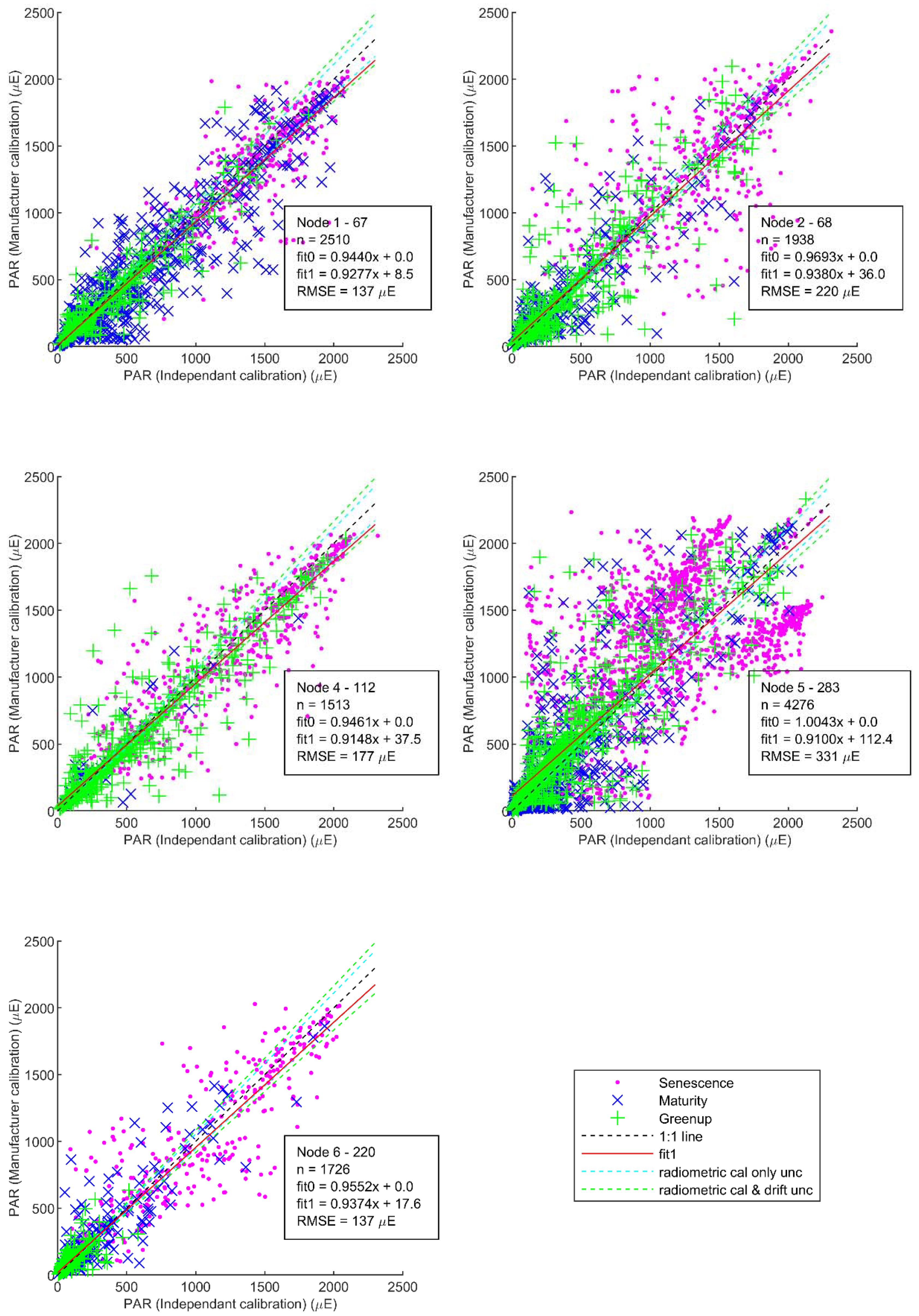
3.1. Sensor Calibration

Figure 4 shows the comparison of the paired sensors, for the five co-located nodes. The first observation is the high variability between the co-located paired sensors, represented by the RMSE values on each plot. In green-up, the PAR values are generally low and closer to the 1:1 line. The maturity and senescence phases show generally higher PAR values, but also a larger scatter, upto a factor 2 different between the co-located identical sensor measurements. The variance is primarily explained by small spatial scale illumination variation from the canopy, and is the subject of the analysis (see Section 3.3. for detailed explanation). For 4 of the 5 nodes [1,2,4,6] the distributions appear normal, with RMSE values between 130 μE and 220 μE [mean PAR ~500 μE] and are suited to a linear model. Node 5 is different, with a higher RMSE of 331 μE, largely due to a distinct bi-modal behavior in the senescence data especially for PAR > 1200 µE. The bi-modal behavior would suggest that one sensor is shadowed when the other is illuminated (and vice versa), suggesting some systematic influence that requires further investigation.

To agree within uncertainties, the fit gradient needs to be 1 ± 0.083, or between 0.917 and 1.083. Table 2 shows the fit gradients, for a forced zero intercept (fit0) and standard linear fit (fit1), together with the percentage deviation in parentheses. For fit0, all nodes agree within uncertainties, whereas for fit1, the gradients for nodes 4 and 5 just exceed this 68% confidence bound. Whether fit0 or fit1 is more appropriate can be debated. Fit0 is more correct given the simple gradient analysis but assumes no bias offset, whereas fit1 allows a physically realistic bias offset. The consistent lower gradient and positive y-intercept for all nodes would possibly suggest an offset component to the drift term. This relationship would indicate that the resident sensors have a reduced response and higher dark offset than the newly installed sensors, which would be the more likely case after 3 years of field deployment, and can be confirmed in future sensor recalibrations. These limits are illustrated in Figure 4, with the fit1 line in red, 1:1 line represented by black dashes, the combined sensor calibration limit √(5%² + 2.5%²) = 5.6% the cyan dashed line and sensor calibration and drift total (8.3%) as the green dashed limits. The agreement at the limit of the total combined uncertainty (but not the combined sensor calibration limit) would suggest that the manufacturer drift estimate of <2% per year is accurate in magnitude, and reinforces the cumulative assumption, i.e., that each year, the drift continues in the same direction.

3.2. Spatial Variability Analysis

For all subsets, the expected reduction in CV occurred with increasing number of sensors, except in the Green up all data case—which needs further investigation (Figure 5). The CV values are higher in the green-up and senescence than in the maturity phenophase. Whereas the green-up and maturity data showed a similar flattening of the curve by 8–10 sensors, whereas the senescence data continued to show noticable reductions in variability beyond 12 sensors. Therefore, at least eight sensors are necessary to characterize the spatial variability of 2-flux fPAR_Domain.

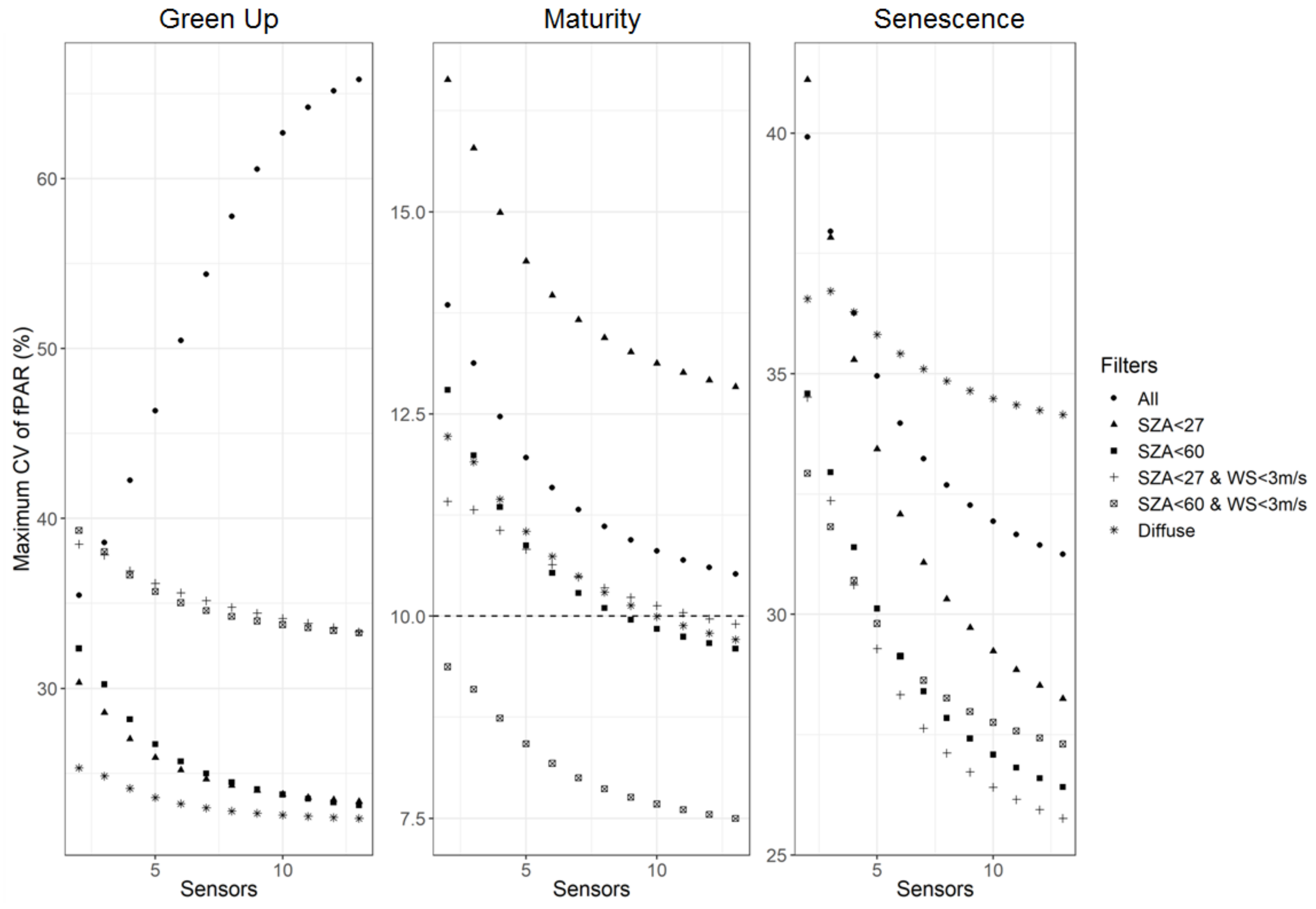
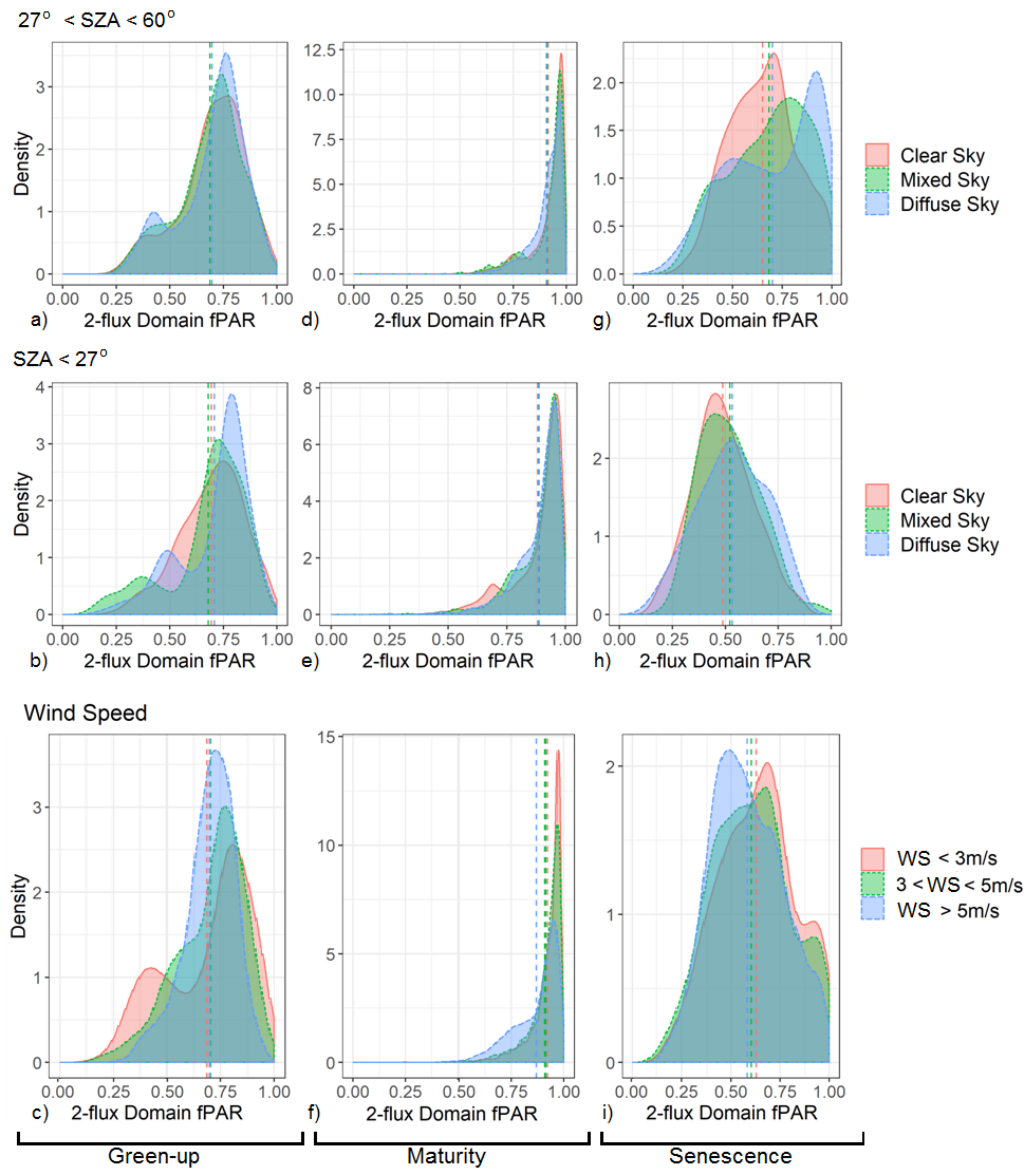
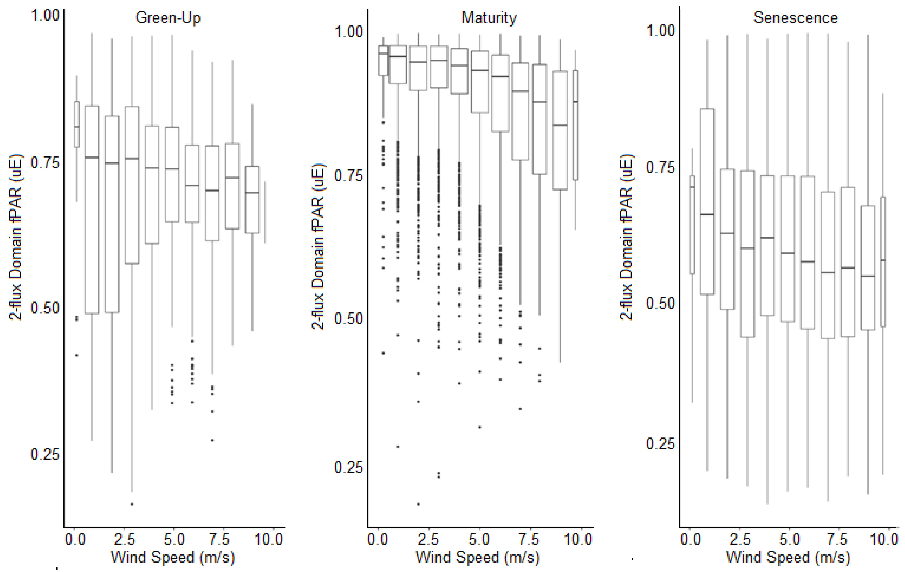
3.3. Variability Due to Environmental Factors by Phenophase

This section subsets the data by phenophase, SZA range, wind speed, and illumination condition to understand the source of the variance seen in Figure 3. Overall our results indicate that skewness and kurtosis of the data indicated that the data were non-normal, therefore, KS tests were performed for each phenophase (green-up, maturity, and senescence) to verify this. When green-up was compared to a normally distributed dataset it was determined to be non-normal (D = 0.60907, p < 2.2 × 10⁻¹⁶); for maturity it was non-normal (D = 0.71465, p < 2.2 × 10⁻¹⁶); and for senescence it was non-normal (D = 0.57942, p < 2.2 × 10⁻¹⁶).

3.3.1. Green-Up

During the green-up phenophase, when 27° < SZA < 60°, there are no significant differences in the central tendencies between different sky conditions (clear sky, CS; mixed sky, MS; and diffuse sky, DS) (Figure 6a) based on the MW test (p > 0.35). There are also similar medians (Mdn) and interquartile ranges (IQR) in each of the fPAR distribution (CS: Mdn = 0.716, IQR = 0.625–0.807/MS: Mdn = 0.725, IQR = 0.615–0.781/DS: Mdn = 0.742, IQR = 0.618–0.794, Figure 6a). During midday conditions where SZA < 27° (Figure 6b), there are significant differences between CS and DS distributions (KS: p = 4.777⁻⁵, MW: p = 0.0434, Cliff d = −0.101), as well as between MS and DS conditions (KS: p = 0.0127); however, there are no significant differences between the median and interquartile ranges in the sky conditions (CS: Mdn = 0.716, IQR = 0.625–0.807; MS: Mdn = 0.725, IQR = 0.615–0.781; DS: Mdn = 0.742, IQR = 0.618–0.794). This significant difference in the MW and KS test but not in the median and IQR may be due to a change in modality between clear and diffuse conditions. The CS conditions result in a unimodal fPAR distribution (skewness = −0.501, kurtosis = −0.122, mode = 0.746, Figure 6a), while mixed and diffuse conditions result in bimodal fPAR distributions (MS: skewness = −1.126, kurtosis = 0.491, modes = 0.356 and 0.732/DS: skewness = −1.039, kurtosis = 0.270, modes = 0.487 and 0.789).

When wind speed is considered during green-up, the greatest wind speeds (WS > 5 m/s) result in lower fPAR variability (mean = 0.699, sd = 0.117, RMSE = 0.00470). When wind-speeds are in the lowest category (WS < 3 m/s), the fPAR variability is the highest (Figure 6), and there is a bimodal distribution (Mdn = 0.758, skewness = −0.589, kurtosis = -0.882, modes = 0.412 & 0.808; Figure 6c). In addition to the change in modality, all fPAR distributions based on wind-speed categories are significantly different based on the KS test (p < 0.05); however, using the MW tests, there is only a significant difference between WS < 3 m/s and WS > 5 m/s (p = 0.0396, Cliff’s d = 0.0763).

3.3.2. Maturity

The fPAR distributions under all-sky conditions, SZA, and wind speeds are heavily skewed in the maturity phenophase (Figure 6d–f). When SZA falls between 27° and 60°, there is a measurable difference between CS and DS in both the KS and MW tests (KS: p = 2.2⁻¹⁶; MW: p = 1.45⁻²⁶, Cliff’s d = 0.180). Detectable differences are also found between MS and DS conditions (KS: p = 3.027⁻⁹, MW: p = 7.95⁻⁸, Cliff’s d = 0.150). In both cases, there is a probability that diffuse conditions will result in lower estimates of 2-flux fPAR_Domain. There are no significant differences in the central tendency or distribution of fPAR between C.S and MS (p > 0.05).

When the SZA < 27°, the modality of fPAR changes as sky conditions move from DS to CS, with the development of a slightly bimodal distribution (Figure 6e). The median fPAR also increases while skewness decreases as conditions clear (DS: Mdn = 0.918/MS: Mdn = 0.927/CS: Mdn = 0.928). This change in mode results in a measurable difference in distribution and central tendencies between CS and DS conditions (KS: p = 3.019⁻⁶; MW: p = 9.46⁻⁴, Cliff’s d = 0.0678). There is no significant difference between MS and either CS or DS conditions at this SZA (p > 0.05).

When looking at wind speeds, all fPAR distributions retain a unimodal distribution. The variability is highest, and the median is lowest under WS > 5 m/s conditions (Mdn = 0.909, IQR = 0.803–0.951). Wind speeds < 3 m/s have the lowest variability and highest median (Mdn = 0.949, IQR = 0.902–0.972; Figure 6f and Figure 7). There are detectable differences between all distributions using the KS test (p < 0.0001). The central tendencies also detectably differ between all wind-speed categories (p < 0.0001), and Cliff’s d indicates that there is a probability that WS <3 m/s or WS between 3–5 m/s will yield higher fPAR estimates than WS > 5 m/s (Cliff’s d = 0.341/0.268).

3.3.3. Senescence

There are differences in the distributions under different external factors, with low SZA producing normal or near-normal distributions, while the SZA between 27° and 60° and wind speeds maintain non-normal distributions (Figure 6g–i). Both the distributions for MS and DS with SZA < 27° are normally distributed according to Shapiro–Wilks (p = 0.226 and p = 0.131, respectively) while CS retains non-normality with a low skewness and kurtosis (p = 1.028⁻⁵, skewness = 0.215, kurtosis = −0.279). Therefore, for this first analysis, Welch’s t-test is used to detect differences. In this case, there is only a detectable difference between CS and DS conditions (t = −2.77, df = 129, p = 0.00641, 95% CI = −0.0744: −0.0124), with no differences found between mixed skies and other sky conditions (p > 0.05).

When SZA increases, skewness increases in both MS and DS conditions and reduces in CS conditions (CS: median = 0.653, skewness = 0.0113, kurtosis = −0.634). Additionally, the distribution becomes bimodal and has the largest variability under diffuse conditions (modes = 0.486 and 0.906; IQR = 0.51–0.98). Overall, there are detectable differences between the central tendencies of CS and both MS and DS conditions (MW test: CS:MS, p = 0.00406, Cliff’s d = 0.101; CS:DS, p = 9.14⁻⁵, Cliff’s d = 0.221). There are also detectable difference between the distributions of all sky conditions (KS test; CS:MS, p = 8.19⁻⁵; CS:DS, p = 1.19⁻¹¹; MS:DS, p = 0.00808).

The greatest difference in central tendencies and distributions between wind speeds is found during senescence (Figure 6i). There are detectable differences between the central tendencies and distribution of fPAR under the lowest and highest wind-speed conditions (KS: p = 1.05⁻⁶; MW: p = 2.46⁻⁶, Cliff’s d = 0.152) with WS < 3 m/s having a higher median fPAR. Both WS < 3 m/s and 3 < WS < 5 m/s have a bimodal distributions with the same modes (modes = 0.923 and 0.704), with a heavier positive tail forming for 3 < WS < 5 m/s (Figure 6i). The difference in the tails between WS < 3 m/s and 3 < WS < 5 m/s creates a weak difference in the central tendencies (MW test: p = 0.0330, Cliff’s d = 0.0808), but not for the cumulative distributions (p = 0.0779). There are also detectable differences between the central tendencies and distribution of 3 < WS < 5 m/s and WS > 5 m/s (KS test: p = 6.48⁻⁴; MW test: p = 8.25⁻³, Cliff’s d = 0.658), with 3 < WS < 5 m/s resulting in higher estimates of 2-flux fPAR_Domain.

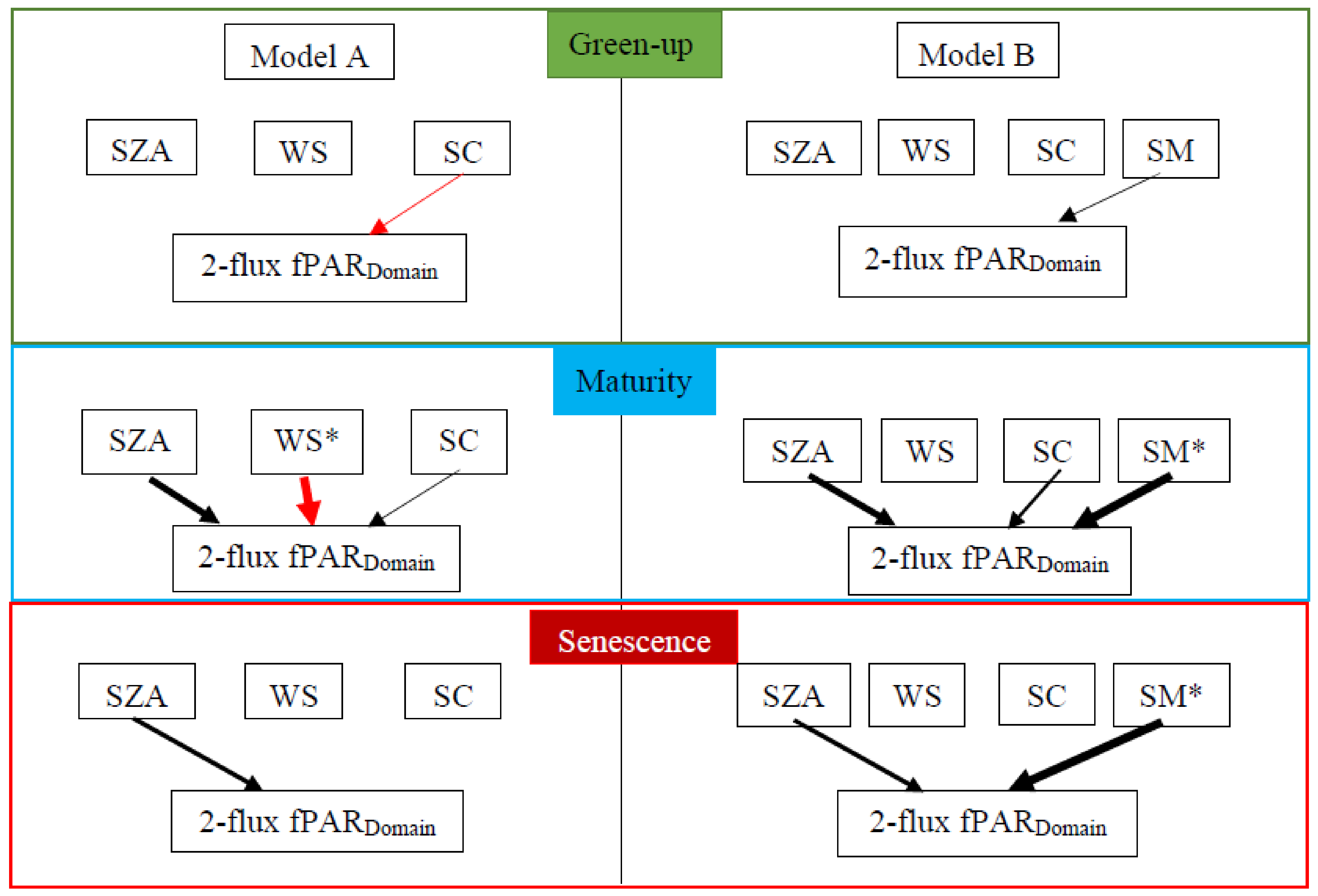
3.4. General Linear Mixed-Effect Models

The first model tested (Figure 8 Model A) includes the variables WS, SZA, and SC and the second (Model B, Figure 8) includes these same variables and soil moisture, SM. Model B consistently outperforms Model A based on the AIC criteria, with Model B having approximately half the AIC score of Model A in all phenophases. During green-up, neither model provided independent variables capable of significantly (p < 0.05) predicting 2-flux fPAR_Domain. During maturity, all independent variables in Model A were significant (p < 0.05), with wind speed having the largest coefficient (−0.155) and SZA (0.0138) and SC (0.000321) having significant but negligible impacts on fPAR prediction (Figure 9). In Model B, WS was no longer significant, both SZA (coef = 0.00888) and SC (coef = 0.000348) retained significance despite their negligible coefficients, and soil moisture became the strongest predictor of 2-flux fPAR_Domain (coef = 0.0709). In senescence Model B displays a similar pattern, as in maturity SM is the strongest predictor of fPAR (coef = 0.0706), although SZA is also significant (coef = 0.0250 being determined significant). In Model A, both WS (coef = −0.0374) and SZA (coef = 0.0282) are significant predictors of 2-flux fPAR_Domain.

4. Discussion

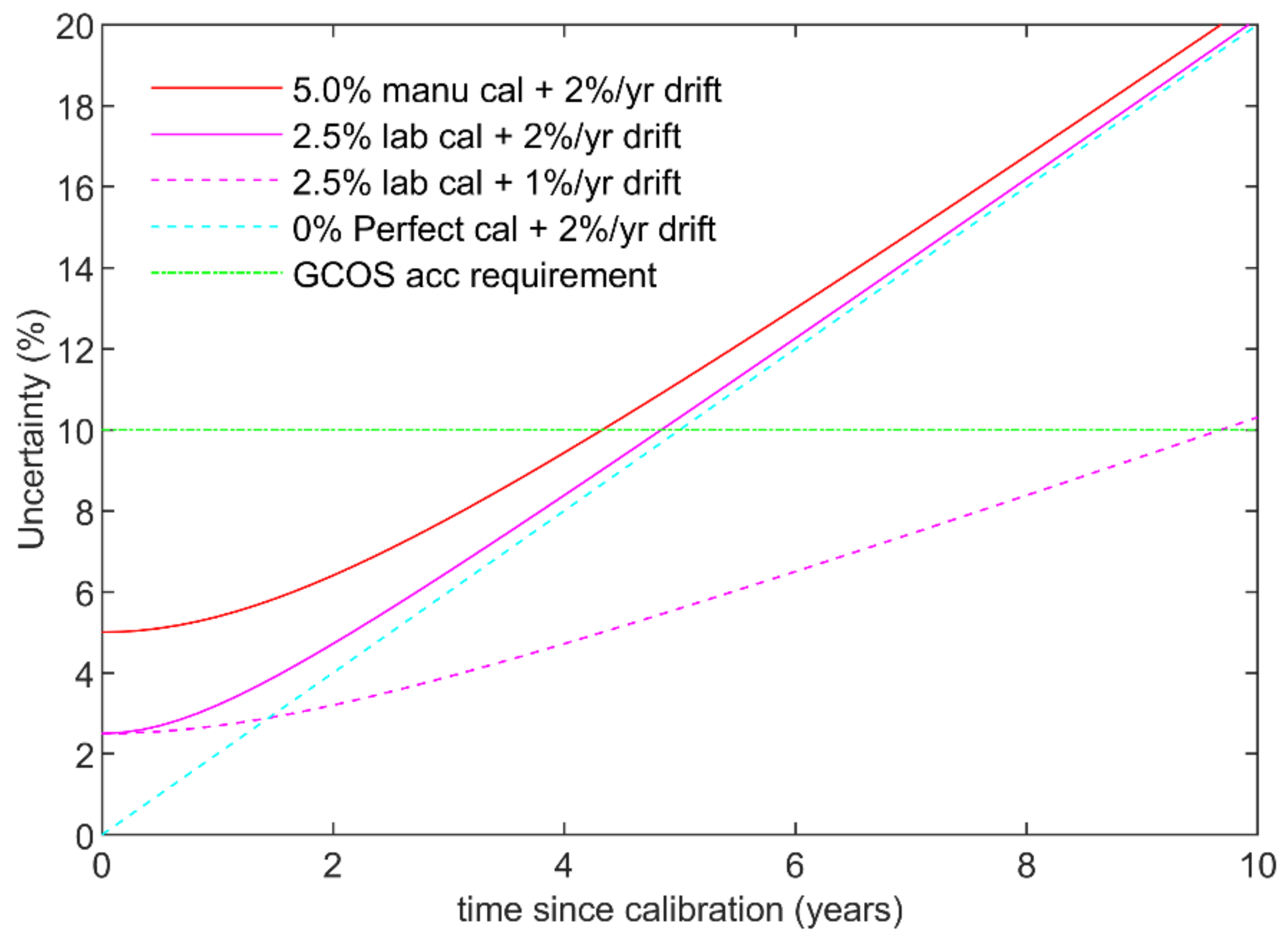
4.1. Calibration Considerations

During the setup of data loggers and PAR sensors, many studies assume that PAR sensor calibrations are valid, and sensors record accurate estimates of PAR [6,56]. The earlier results show that the paired sensors agree within uncertainties, but show the drift term to be sigificant. It is not uncommon for the calibration term to be taken into account and the effect of drift ignored. Figure 8 shows the combined uncertainty, calibration, and drift term over time from the date of calibration. The red and magenta solid lines show the case for the manufacturer-calibrated (5% (k = 1)) and independently calibrated (2.5% (k = 1)) cases, both with a 2% per year drift. Although the initial calibration is better (more accurate) for the independent case, the drift term starts to dominate after a couple of years. The 10% uncertainty crossing for the 2.5% radiometric calibration case is 4 years and 10 months, whereas for the 5% radiometric calibration it is 4 years and 4 months. The better calibration accuracy only buys 6 months of extended field deployment time. The cyan dashed line shows the case for ‘perfect’ 0% radiometric calibration, i.e., 2% per year for 5 years, to reach 10% uncertainty. The conclusion is not that the radiometric sensor calibration accuracy is irrelevant, but that with a dominant drift term its contribution is diminished when considering long-term monitoring networks.

For long-term monitoring sites, using sensors with these charcateristics, the drift term will determine the recalibration requirement to maintain calibration within a defined requirement. For instance, to meet the GCOS requirement of calibration accuracy <10%, the sensors will need to be recalibrated every 4 years (less than 4 years and 4 months with a manufacturer calibration) [16,48]. However, the GCOS stability requirement of 3% [39] puts a more stringent requirement on instrument design, and for the current Apogee sensors, shortens the recalibration period to 18 months. The most immediate activity to improve long-term montioring sites would be to address the drift term to improve long-term stability. The magenta dashed line in Figure 8 show a 2.5% radiometric calibration for a 1% per year drift sensor, lengthening the required time between recalibration although the longer-term aim should be to have drift terms << 1% per year. The manufacturer stated drift of <2% per year is an upper limit (although the earlier analysis concluded that is was a reasonable estimate for the sensors at this field site) and characterizing the drift term over a number of repeat calibrations would provide a more specific recalibration need for a particular sensor (although concerns over a change in drift behavior of an aging sensor may result in the prudent action to maintain a regular calibration schedule).

Additionally, Santa Rosa National Park exhibits a high degree of spatial variability in all phenophases.

4.2. Influence of Environmental Conditions on the 2-Flux fPAR GLME

Of the two variables indicative of illumination conditions, SZA exhibits a higher significance in the prediction of 2-flux fPAR_Domain during maturity and senescence in the GLME. Additionally, larger SZA values (>27°) results in spatial homogenization. This homogenization lowers the variability of the understory light environment, but also misses the canopy heterogeneity, especially during transitional phenophases. The predictive significance and reduced heterogeneity of fPAR at higher SZA may be due to a convergence of fPAR across all LAI values at an SZA of 60° [6]. This convergence is especially crucial during lower LAI periods (LAI < 4; [6]) because as the path of direct radiation lengthens with an increased SZA, there is an increased chance of interception by leaves, which inflates fPAR. Other studies have found that estimates of fPAR made under direct radiation, at times of nadir observations, can be underestimated by up to 10% when LAI < 2 as it often can be during these transitional phenophases, especially during green-up [53].

Regardless of phenophase and SZA, clear-sky conditions and diffuse-sky conditions always have differences in their central tendencies and distributions. Additionally, clear-sky conditions have a decreased standard deviation, root mean square error, and median compared to diffuse-sky conditions during transitional phenophases, while the opposite is true during maturity. Other studies find that diffuse radiation is more readily absorbed by photosynthesizing material [6,31]. Not only does diffuse radiation permit the deeper penetration of photons, but these conditions promote increased light-use efficiency of plant canopies and decrease the frequency of photosynthetic saturation [31,56]. Therefore, it should be anticipated that during diffuse conditions that only the effect of the canopy condition is being measured, and that the amount of PAR absorbed increases proportional to LAI, yielding both increased 2-flux fPAR_Domain estimates and an accurate reflection of the leaf area observed during those periods [57,58]. The bimodal distributions exhibited under diffuse sky conditions are also more reflective of the 2-flux fPAR_Domain values expected under variable LAI values [6,53]. A bimodal distribution alone could also explain why SCs were not as significant to the GLME (Figure 7), as the bimodality increases the RMSE of the relationship between SC and 2-flux fPAR_Domain.

Wind speeds greater than 5 m/s during periods of canopy maturity were found to increase the spatial variability of the understory light environment, causing an underestimation in the 2-flux fPAR reported. Regardless of this, WS did not present any explanatory power in the GLME except for Model A during maturity. These findings replicate those found in the coniferous-dominated forest [24]. High wind speeds are found at the end of maturity and throughout senescence before receding with the start of green-up. The underestimation of 2-flux fPAR_Domain during these high-wind periods could be due to changes in leaf angle orientation. As wind speed increases, leaves change from planophile to erectophile or plagiophile, permitting photons to penetrate deeper into the canopy decreasing the fraction of absorbed PAR in the canopy [59,60]. Model predictions of this canopy behavior and the resulting impact on fPAR [59] are similar to the behavior exhibited by the SRNP EMSS canopy during maturity as wind speeds increase.

The significance of SM found in all phenophases reinforces the well-established understanding of a water-limited ecosystem [61,62,63,64] with precipitation and soil moisture controlling green-up, and influencing the photosynthetic capacities of tree canopies relative to the water available in the area [65]. Additionally, increased SM occurs concurrently with the presence of lianas, which are known to decrease the canopy openness providing shade for the understory below [66]. Lianas also tend to delay their leaf abscission during senescence [67], increasing LAI for that specific area and consequently increasing fPAR.

Overall, due to the overestimation during phenological maturity of 2-flux fPAR under clear sky conditions, and the influence of SZA on 2-flux fPAR estimation, ground data for validating satellite-derived fPAR should be acquired when diffuse light conditions persist, shortly before or after satellite overpass [24]. This type of procedure requires permanent monitoring sites, which is made possible by the WSN technology utilized in this study. Furthermore, if WSN technology is to continue to be employed, it should be coupled with time-lapse or periodic photography campaigns linking a physical phenomenon with the observed phenomenon in the WSN fPAR time-series.

5. Conclusions

This study was designed to evaluate the methodological procedures surrounding collecting ground fPAR fluxes to validate satellite fPAR products. As the first study of its kind in the tropical dry forest, sensor networks, and external variables were tested. Overall, we find that the sensor drift term dominates, and requires recalibration every 4 years, to remain within a 10% calibration requirement. Additionally, we find that to reduce variability these measurements should be collected in the maturity phenophase with a network of at least eight sensors. The lowest variance scenario is for measurements with diffuse light conditions or SZA > 27°, and wind-speeds < 5 m/s. Utilizing the comparisons and results found in this study, the findings presented here could be used in the development of experimental designs in tropical areas, which exhibit substantially less representation in the validation of satellite-derived fPAR products.

A permanent wireless sensor network, in combination with local meteorological towers, can be used to further quantify the sources of uncertainty and variability of fPAR in forest environments. Sites such as these are instrumental for the progression of satellite-derived fPAR products over forested areas, especially in tropical forests where very few validation sites exist. As satellite-derived fPAR products continue to expand, there will be a need for field validation sites to assess the influence of various environmental variables and to determine how assumptions differ by biome. No other method permits the high temporal and spatial resolution necessary for the validation of upcoming decametric satellite products and, as such, this method needs to be considered in the validation of these upcoming satellite products. Further research, to study the potential limits of our approach into the effects of soil reflectance and top-of-canopy reflectance on fPAR during times of canopy turbidity should be assessed moving forward, especially during short-term sampling.

References

1. McDowell, N.G.; Coops, N.C.; Beck, P.S.A.; Chambers, J.Q.; Gangodagamage, C.; Hicke, J.A.; Huang, C.; Kennedy, R.; Krofcheck, D.J.; Litvak, M.; et al. Global satellite monitoring of climate-induced vegetation disturbances. Trends Plant Sci. 2015, 20, 114–123. [Google Scholar] [CrossRef] [PubMed] [Green Version]
2. Claverie, M.; Vermote, E.F.; Weiss, M.; Baret, F.; Hagolle, O.; Demarez, V. Validation of coarse spatial resolution LAI and FAPAR time series over cropland in southwest France. Remote Sens. Environ. 2013, 139, 216–230. [Google Scholar] [CrossRef]
3. Gower, S.T.; Kucharik, C.J.; Norman, J.M. Direct and Indirect Estimation of Leaf Area Index, fAPAR, and Net Primary Production of Terrestrial Ecosystems. Remote Sens. Environ. 1999, 70, 29–51. [Google Scholar] [CrossRef]
4. Myneni, R.; Ramakrishna, R.; Nemani, R.; Running, S. Estimation of global leaf area index and absorbed par using radiative transfer models. IEEE Trans. Geosci. Remote Sens. 1997, 35, 1380–1393. [Google Scholar] [CrossRef] [Green Version]
5. Myneni, R.B.; Knyazikhin, Y.; Privette, J.L.; Running, S.W.; Nemani, R.; Zhang, Y.; Tian, Y.; Wang, Y.; Morissette, J.T.; Glassy, J.; et al. MODIS. Leaf Area Index (LAI) And Fraction Of Photosynthetically Active Radiation Absorbed By Vegetation (FPAR) Product. Modis Atbd 1999, Version 4, 130. Available online: http://eospso.gsfc.nasa.gov/atbd/modistables.html (accessed on 1 September 2018).
6. Li, W.; Fang, H. Estimation of direct, diffuse, and total FPARs from Landsat surface reflectance data and ground-based estimates over six FLUXNET sites. J. Geophys. Res. Biogeosci. 2015, 120, 96–112. [Google Scholar] [CrossRef]
7. Gobron, N.; Pinty, B.; Aussedat, O.; Chen, J.M.; Cohen, W.B.; Fensholt, R.; Gond, V.; Huemmrich, K.F.; Lavergne, T.; Mélin, F.; et al. Evaluation of fraction of absorbed photosynthetically active radiation products for different canopy radiation transfer regimes: Methodology and results using Joint Research Center products derived from SeaWiFS against ground-based estimations. J. Geophys. Res. Earth Surf. 2006, 111, D13. [Google Scholar] [CrossRef]
8. Thomas, V.; Finch, D.; McCaughey, J.; Noland, T.; Rich, L.; Treitz, P. Spatial modelling of the fraction of photosynthetically active radiation absorbed by a boreal mixedwood forest using a lidar–hyperspectral approach. Agric. For. Meteorol. 2006, 140, 287–307. [Google Scholar] [CrossRef]
9. Chen, J. Canopy architecture and remote sensing of the fraction of photosynthetically active radiation absorbed by boreal conifer forests. IEEE Trans. Geosci. Remote Sens. 1996, 34, 1353–1368. [Google Scholar] [CrossRef]
10. Widlowski, J.-L. On the bias of instantaneous FAPAR estimates in open-canopy forests. Agric. For. Meteorol. 2010, 150, 1501–1522. [Google Scholar] [CrossRef]
11. Bondeau, A.; Kicklighter, D.W.; Kaduk, J. Model Intercomparison. Comparing global models of terrestrial net primary productivity (NPP): Importance of vegetation structure on seasonal NPP estimates. Glob. Chang. Biol. 1999, 5, 35–45. [Google Scholar] [CrossRef]
12. Liu, R.; Sun, J.; Wang, J.; Li, X.; Yang, F.; Chen, P. Study of remote sensing based parameter uncertainty in production efficiency models state key laboratory of resources and environmental information systems. In Proceedings of the 2010 IEEE International Geoscience and Remote Sensing Symposium, Honolulu, HI, USA, 25–30 July 2010; pp. 3303–3306. [Google Scholar]
13. Madani, N.; Kimball, J.S.; Running, S.W. Improving Global Gross Primary Productivity Estimates by Computing Optimum Light Use Efficiencies Using Flux Tower Data. J. Geophys. Res. Biogeosci. 2017, 122, 2939–2951. [Google Scholar] [CrossRef]
14. Zhang, R.; Zhou, Y.; Luo, H.; Wang, F.; Wang, S. Estimation and Analysis of Spatiotemporal Dynamics of the Net Primary Productivity Integrating Efficiency Model with Process Model in Karst Area. Remote Sens. 2017, 9, 477. [Google Scholar] [CrossRef] [Green Version]
15. Zhu, Q.; Zhao, J.; Zhu, Z.; Zhang, H.; Zhang, Z.; Guo, X.; Bi, Y.; Sun, L. Remotely Sensed Estimation of Net Primary Productivity (NPP) and Its Spatial and Temporal Variations in the Greater Khingan Mountain Region, China. Sustainability 2017, 9, 1213. [Google Scholar] [CrossRef] [Green Version]
16. Nightingale, J.; Schaepman-Strub, G.; Nickeson, J. Assessing satellite-derived land product quality for Earth system science applications: Overview of the CEOS LPV sub-group. In Proceedings of the Earth Observation for Land-Atmosphere Interaction Science Conference, Rome, Italy, 3–5 November 2010. [Google Scholar]
17. Carrara, A.; Kolari, P.; De Beeck, M.O.; Arriga, N.; Berveiller, D.; Dengel, S.; Ibrom, A.; Merbold, L.; Rebmann, C.; Sabbatini, S.; et al. Radiation measurements at ICOS ecosystem stations. Int. Agrophys. 2018, 32, 589–605. [Google Scholar] [CrossRef]
18. D’Odorico, P.; Gonsamo, A.; Pinty, B.; Gobron, N.; Coops, N.; Mendez, E.; Schaepman, M.E. Intercomparison of fraction of absorbed photosynthetically active radiation products derived from satellite data over Europe. Remote Sens. Environ. 2014, 142, 141–154. [Google Scholar] [CrossRef]
19. Majasalmi, T.; Stenberg, P.; Rautiainen, M. Comparison of ground and satellite-based methods for estimating stand-level fPAR in a boreal forest. Agric. For. Meteorol. 2017, 232, 422–432. [Google Scholar] [CrossRef]
20. Nestola, E.; Sánchez-Zapero, J.; Latorre, C.; Mazzenga, F.; Matteucci, G.; Calfapietra, C.; Camacho, F. Validation of PROBA-V GEOV1 and MODIS C5 & C6 fAPAR Products in a Deciduous Beech Forest Site in Italy. Remote Sens. 2017, 9, 126. [Google Scholar] [CrossRef] [Green Version]
21. Senna, M.C.A.; Costa, M.H.; Shimabukuro, Y.E. Fraction of photosynthetically active radiation absorbed by Amazon tropical forest: A comparison of field measurements, modeling, and remote sensing. J. Geophys. Res. Earth Surf. 2005, 110, G01008. [Google Scholar] [CrossRef] [Green Version]
22. Stenberg, P.; Mõttus, M.; Rautiainen, M. Photon recollision probability in modelling the radiation regime of canopies—A review. Remote Sens. Environ. 2016, 183, 98–108. [Google Scholar] [CrossRef]
23. Van Der Zande, D.; Stuckens, J.; Verstraeten, W.W.; Muys, B.; Coppin, P. Assessment of Light Environment Variability in Broadleaved Forest Canopies Using Terrestrial Laser Scanning. Remote Sens. 2010, 2, 1564–1574. [Google Scholar] [CrossRef] [Green Version]
24. Putzenlechner, B.; Marzahn, P.; Kiese, R.; Ludwig, R.; Sanchez-Azofeifa, A. Assessing the variability and uncertainty of two-flux FAPAR measurements in a conifer-dominated forest. Agric. For. Meteorol. 2018, 264, 149–163. [Google Scholar] [CrossRef]
25. Steinberg, D.; Goetz, S.; Hyer, E. Validation of MODIS. F/sub PAR/products in boreal forests of Alaska. IEEE Trans. Geosci. Remote Sens. 2006, 44, 1818–1828. [Google Scholar] [CrossRef]
26. Li, W.; Weiss, M.; Waldner, F.; Defourny, P.; Demarez, V.; Morin, D.; Hagolle, O.; Baret, F. A Generic Algorithm to Estimate LAI, FAPAR and FCOVER Variables from SPOT4_HRVIR and Landsat Sensors: Evaluation of the Consistency and Comparison with Ground Measurements. Remote Sens. 2015, 7, 15494–15516. [Google Scholar] [CrossRef] [Green Version]
27. Fensholt, R.; Sandholt, I.; Rasmussen, M.S. Evaluation of MODIS LAI, fAPAR and the relation between fAPAR and NDVI in a semi-arid environment using in situ measurements. Remote Sens. Environ. 2004, 91, 490–507. [Google Scholar] [CrossRef]
28. Pinty, B.; Jung, M.; Kaminski, T.; Lavergne, T.; Mund, M.; Plummer, S.; Thomas, E.; Widlowski, J.-L. Evaluation of the JRC-TIP 0.01° products over a mid-latitude deciduous forest site. Remote Sens. Environ. 2011, 115, 3567–3581. [Google Scholar] [CrossRef]
29. Ahl, D.E.; Gower, S.T.; Burrows, S.N.; Shabanov, N.V.; Myneni, R.; Knyazikhin, Y. Monitoring spring canopy phenology of a deciduous broadleaf forest using MODIS. Remote Sens. Environ. 2006, 104, 88–95. [Google Scholar] [CrossRef] [Green Version]
30. Pickett-Heaps, C.A.; Canadell, J.G.; Briggs, P.R.; Gobron, N.; Haverd, V.; Paget, M.; Pinty, B.; Raupach, M.R. Evaluation of six satellite-derived Fraction of Absorbed Photosynthetic Active Radiation (FAPAR) products across the Australian continent. Remote Sens. Environ. 2014, 140, 241–256. [Google Scholar] [CrossRef]
31. Gu, L.; Baldocchi, D.; Verma, S.B.; Black, T.A.; Vesala, T.; Falge, E.M.; Dowty, P.R. Advantages of diffuse radiation for terrestrial ecosystem productivity. J. Geophys. Res. Earth Surf. 2002, 107, ACL 2-1–ACL 2-23. [Google Scholar] [CrossRef] [Green Version]
32. Leuchner, M.; Hertel, C.; Menzel, A. Spatial variability of photosynthetically active radiation in European beech and Norway spruce. Agric. For. Meteorol. 2011, 151, 1226–1232. [Google Scholar] [CrossRef]
33. Shabanov, N.; Wang, Y.; Buermann, W.; Dong, J.; Hoffman, S.; Smith, G.; Tian, Y.; Knyazikhin, Y.; Myneni, R. Effect of foliage spatial heterogeneity in the MODIS LAI and FPAR algorithm over broadleaf forests. Remote Sens. Environ. 2003, 85, 410–423. [Google Scholar] [CrossRef] [Green Version]
34. Portillo-Quintero, C.; Sánchez-Azofeifa, G. Extent and conservation of tropical dry forests in the Americas. Biol. Conserv. 2010, 143, 144–155. [Google Scholar] [CrossRef]
35. Pastorello, G.Z.; Sanchez-Azofeifa, G.A.; Nascimento, M.A. Enviro-Net: A Network of Ground-based Sensors for Tropical Dry Forests in the Americas. Sensors 2011, 11, 6454–6479. [Google Scholar] [CrossRef] [PubMed]
36. Rawat, P.; Singh, K.D.; Chaouchi, H.; Bonnin, J.M. Wireless sensor networks: A survey on recent developments and potential synergies. J. Supercomput. 2014, 68, 1–48. [Google Scholar] [CrossRef]
37. Sanchez-Azofeifa, A.; Guzmán, J.A.; Campos, C.A.; Castro, S.; Garcia-Millan, V.; Nightingale, J.; Rankine, C. Twenty-first century remote sensing technologies are revolutionizing the study of tropical forests. Biotropica 2017, 49, 604–619. [Google Scholar] [CrossRef]
38. S’nchez-Azofeifa, G.A.; Rankine, C.; Santo, M.M.D.E.; Fatland, R.; Garcia, M. Wireless Sensing Networks for Environmental Monitoring: Two Case Studies from Tropical Forests. In Proceedings of the 2011 IEEE Seventh International Conference on eScience, Stockholm, Sweden, 5–8 December 2011; pp. 70–76. [Google Scholar] [CrossRef]
39. World Meteorological Organization. Systematic Observation Requirements for Satellite-Based Data Products for Climate 2011 Update Supplemental Details to the Satellite-Based Component of the Implementation Plan; WMO: Geneva, Swizerland, 2011. [Google Scholar]
40. Janzen, D.H. Costa Rica’s Area de Conservación Guanacaste: A long march to survival through non-damaging biodevelopment. Biodiversity 2000, 1, 7–20. [Google Scholar] [CrossRef]
41. Janzen, D.H.; Hallwachs, W. Biodiversity Conservation History and Future in Costa Rica: The Case of Área de Conservación Guanacaste (ACG). Costa Rican Ecosyst. 2016, 290, 300. [Google Scholar]
42. Kalacska, M.; Sanchez-Azofeifa, A.; Calvo-Alvarado, J.C.; Quesada, M.; Rivard, B.; Janzen, D. Species composition, similarity and diversity in three successional stages of a seasonally dry tropical forest. For. Ecol. Manag. 2004, 200, 227–247. [Google Scholar] [CrossRef]
43. Sanchez-Azofeifa, G.A.; Kalacska, M.; Quesada, M.; Calvo-Alvarado, J.C.; Nassar, J.M.; Rodriguez, J.P. Need for Integrated Research for a Sustainable Future in Tropical Dry Forests. Conserv. Biol. 2005, 19, 285–286. [Google Scholar] [CrossRef]
44. Rankine, C.J. Monitoring Seasonal and Secondary Succession Processes in Deciduous Forests Using Near-Surface Optical Remote Sensing and Wireless Sensor Networks. Ph.D. Thesis, University of Alberta, Edmonton, AB, Canada, 2016; p. 167. [Google Scholar] [CrossRef]
45. Younis, M.; Akkaya, K. Strategies and techniques for node placement in wireless sensor networks: A survey. Ad Hoc Netw. 2007, 6, 621–655. [Google Scholar] [CrossRef]
46. Quantum Sensor Models SQ-100 and SQ-300 Series (Including S.S. Models); Apogee Instruments Rev: Logan, UT, USA, 2019; 20p.
47. Apogee Quantum Sensor Calibration Certificate; Apogee Instruments: Logan, UT, USA, 2019.
48. JCGM Evaluation of Measurement Data—Guide to the Expression of Uncertainty in Measurement (Évaluation des Données de Mesure—Guide Pour l’Expression de l’Incertitude de Mesure). 2008. Available online: https://www.bipm.org/documents/20126/2071204/JCGM_100_2008_E.pdf/cb0ef43f-baa5-11cf-3f85-4dcd86f77bd6 (accessed on 1 September 2018).
49. Walter, I.A.; Allen, R.; Elliot, R.; Itenfisu, D.; Brown, P.; Jensen, M.E.; Mecham, B.; Howell, T.A.; Snyder, R.; Eching, S.; et al. The asce standardized reference evapotranspiration equation environmental and water resources institute of the American society of civil engineers standardization of reference evapotranspiration task committee. Am. Soc. Civ. Eng. 2002, 1, 1–51. [Google Scholar]
50. Lange, M.; Doktor, D. phenex: Auxiliary Functions for Phenological Data Analysis. R Package Version 1.4-5. 2017. Available online: https://cran.r-project.org/web/packages/phenex/index.html (accessed on 1 September 2018).
51. Cliff, N. Dominance statistics: Ordinal analyses to answer ordinal questions. Psychol. Bull. 1993, 114, 494. [Google Scholar] [CrossRef]
52. Chadwick, R.; Good, P.; Martin, G.; Rowell, D.P. Large rainfall changes consistently projected over substantial areas of tropical land. Nat. Clim. Chang. 2015, 6, 177–181. [Google Scholar] [CrossRef]
53. Kalacska, M.; Calvo-Alvarado, J.C.; Sanchez-Azofeifa, G.A. Calibration and assessment of seasonal changes in leaf area index of a tropical dry forest in different stages of succession. Tree Physiol. 2005, 25, 733–744. [Google Scholar] [CrossRef] [Green Version]
54. Zelazowski, P.; Malhi, Y.; Huntingford, C.; Sitch, S.; Fisher, J. Changes in the potential distribution of humid tropical forests on a warmer planet. Philos. Trans. R. Soc. Lond. Ser. A Math. Phys. Eng. Sci. 2011, 369, 137–160. [Google Scholar] [CrossRef]
55. Wang, H. Extending the Linear Model with R: Generalized Linear, Mixed Effects and Nonparametric Regression Models Edited by Faraway J. J. Biom. 2006, 62, 1278. [Google Scholar] [CrossRef]
56. Majasalmi, T. Estimation of Leaf Area Index and the Fraction of Absorbed Photosynthetically Active Radiation in a Boreal; University of Helsinki: Helsinki, Finland, 2015; ISBN 9789516514638. [Google Scholar]
57. Chazdon, R.L.; Fetcher, N. Photosynthetic Light Environments in a Lowland Tropical Rain Forest in Costa Rica. J. Ecol. 1984, 72, 553–564. [Google Scholar] [CrossRef]
58. Vierling, L.A.; Wessman, C.A. Photosynthetically active radiation heterogeneity within a monodominant Congolese rain forest canopy. Agric. For. Meteorol. 2000, 103, 265–278. [Google Scholar] [CrossRef]
59. Asner, G.P.; Wessman, C.A. Scaling PAR absorption from the leaf to landscape level in spatially heterogeneous ecosystems. Ecol. Model. 1997, 103, 81–97. [Google Scholar] [CrossRef]
60. Verhoef, W. Light scattering by leaf layers with application to canopy reflectance modeling: The SAIL model. Remote Sens. Environ. 1984, 16, 125–141. [Google Scholar] [CrossRef] [Green Version]
61. Campos, F.A. A Synthesis of Long-Term Environmental Change in Santa Rosa, Costa Rica. In Primate Life Histories, Sex Roles, and Adaptability; Springer: Cham, Switzerland, 2018; pp. 331–358. [Google Scholar] [CrossRef]
62. Castillo-Núñez, M.; Sánchez-Azofeifa, G.A.; Croitoru, A.; Rivard, B.; Calvo-Alvarado, J.; Dubayah, R.O. Delineation of secondary succession mechanisms for tropical dry forests using LiDAR. Remote Sens. Environ. 2011, 115, 2217–2231. [Google Scholar] [CrossRef]
63. Janzen, D.H. Tropical dry forests. Biodiversity 1988, 15, 130–137. [Google Scholar]
64. Sanchez-Azofeifa, G.A.; Quesada, M.; Rodriguez, J.P.; Nassar, J.M.; Stoner, K.E.; Castillo, A.; Garvin, T.; Zent, E.L.; Calvo-Alvarado, J.C.; Kalacska, M.E.; et al. Research Priorities for Neotropical Dry Forests. Biotropica 2005, 37, 477–485. [Google Scholar] [CrossRef]
65. Hwang, T.; Gholizadeh, H.; Sims, D.A.; Novick, K.A.; Brzostek, E.R.; Phillips, R.P.; Roman, D.T.; Robeson, S.; Rahman, A.F. Capturing species-level drought responses in a temperate deciduous forest using ratios of photochemical reflectance indices between sunlit and shaded canopies. Remote Sens. Environ. 2017, 199, 350–359. [Google Scholar] [CrossRef]
66. Sánchez-Azofeifa, G.A.; Kalácska, M.; Espírito-Santo, M.M.D.; Fernandes, G.W.; Schnitzer, S. Tropical dry forest succession and the contribution of lianas to wood area index (WAI). For. Ecol. Manag. 2009, 258, 941–948. [Google Scholar] [CrossRef]
67. Cai, Z.-Q.; Schnitzer, S.A.; Bongers, F. Seasonal differences in leaf-level physiology give lianas a competitive advantage over trees in a tropical seasonal forest. Oecologia 2009, 161, 25–33. [Google Scholar] [CrossRef] [Green Version]
Figure 1. The location of the Santa Rosa National Park—Environmental Monitoring Super Site (SRNP-EMSS), Guanacaste, Costa Rica. Network 1 refers to the WSN that is employed in the creation of the in-situ fPAR product.
Remotesensing 14 02752 g001
Figure 2. Schematics of the distribution of the nodes at the wireless sensor network used in this study at the Santa Rosa National Park—Environmental Monitoring Super Site (SRNP-EMSS), Guanacaste, Costa Rica. Black square nodes (112, 68, 67, 220 and 283) have co-located PAR nodes. Empty white circles (72, 74, 75, 79, 80, 86, 100, and 126) have just one PAR sensor.
Remotesensing 14 02752 g002
Figure 3. Breakdown of the 2-flux fPAR time-series into phenophases. Phenophases were determined using the R package “Phenex”(phenex_1.4–5.tar.gz) and based on the local thresholds determined per year.
Remotesensing 14 02752 g003
Figure 4. A one-to-one comparison between the co-located PAR sensor pairs. In all plots, the red line indicates the linear regression (fit1) between the sensors at each node, whereas the black dotted line indicates a 1:1 line. The x axis labeled “independent calibration” refers to NPL calibrated sensors, and the y-axis, labeled ‘manufacturer calibration’ refers to the Apogee calibrated sensors. The green symbols are ‘green-up’, blue are ‘maturity’, and magenta are ‘senescence’. For each node, the inner cyan dashed lines denote the combined calibration uncertainty range, whereas the outer green dashed lines are the calibration and drift terms. The type ft0 corresponds to a 0 forced linear regression, and ft1 corresponds to a 1:1 forced linear regression.
Remotesensing 14 02752 g004
Figure 5. The coefficient of variation in the 2-flux domain fPAR is based on the number of sensors, data filtering, and phenophase. During green-up (left) the diffuse light has the lowest CV; however, no number of sensors reduces variation to below the 10% threshold. During maturity (center), two sensors are needed to meet the threshold at a high SZA and low wind speed; however, eight sensors are required in other circumstances. In senescence (right), there is no number of sensors or amount of filtering that will reach the threshold, but a low SZA and wind speed results in the lowest CV.
Remotesensing 14 02752 g005
Figure 6. The influence of solar zenith angles, sky conditions, and wind speed on the distribution of 2-flux domain fPAR. These three sets of panels are split into the respective phenophases: (a,b), and (c) green-up; (df) maturity; (gi) senescence. The upper and middle panels assess the fPAR distributions based on different SZA and sky conditions. The lower panel assesses the distribution of fPAR based on different wind speeds.
Remotesensing 14 02752 g006
Figure 7. The influence of wind speed on the estimation of 2-flux fPARDomain by phenophase: (left) green-up; (center) maturity; (right) senescence. Boxplots represent the IQR of each set of measurements, while wind speed is broken into 1ms−1 groupings for the analysis.
Remotesensing 14 02752 g007
Figure 8. The influence of independent variables on 2-flux fPARDomain for two GLME models. In every instance, Model B, which included the variable soil moisture (S.M.) had an AIC score half the magnitude of Model A’s. An asterisk (*) indicates those variables with significant (p < 0.05) influence. Black arrows indicate positive coefficients, red arrows indicate negative coefficients, with the thickness of the arrow indicating the relative effect of the variable, compared to other variables of significance. Arrows associated with variables that do not display the * symbol are variables selected by the stepwise logistic regression but that did not significantly impact the results of the GLME.
Remotesensing 14 02752 g008
Figure 9. Sensor uncertainty over time for a range of radiometic calibration accruacies and drift term magnitudes. All uncertainties are assumed to be k = 1, please refer to Equation (2).
Remotesensing 14 02752 g009