Characterizing Spatial Patterns of the Response Rate of Vegetation Green-Up Dates to Land Surface Temperature in Beijing, China (2001–2019)

Abstract

The phenology indicator of vegetation green-up dates (GUD) is prone to being affected by changes in temperature. However, the influencing degree of urbanization-induced temperature warming on vegetation GUDs among different vegetation species along the urban-rural gradient remains inadequately described. In this study, based on the long-term (2001–2019) satellite-derived vegetation GUDs and nighttime land surface temperature (LST) of forests, grasslands, and croplands along the urban-rural gradient with Beijing (China) as a case study area, the responses of vegetation GUDs to temperature changes were quantitatively analyzed, taking into account the vegetation types and distances away from the urban domain. The results show that (1) long-term GUDs and LST are significantly negatively correlated, characterized by a weaker significant correlation near the urban area when compared with its surrounding areas, with the greatest absolute linear correlation coefficients (r) happening at rings 32 km (r_max = −0.93, forests), 20 km and 48 km (r_max = −0.83, grasslands), and 34 km (r_max = −0.82, croplands), respectively; (2) the magnitude of change in GUDs over the past 19 year (2001–2019) are significantly positively correlated with these in LST near the urban area, demonstrating a distance-decay trend, with the greatest advance in GUDs occurring at the ring nearest the urban area, by about 20 days (forests), 24.5 days (grasslands), and 15.6 days (croplands), respectively; (3) the spatial pattern of the response rate of GUDs change to LST change (days K⁻¹) also showed a declining trend with distance, with GUD advanced by 6.8 days K⁻¹ (forests), 7.5 days K⁻¹ (grasslands), and 4.9 days K⁻¹ (croplands) at the closest ring to the urban, decreasing to about 2.3 days K⁻¹ (48 km), 4.1 days K⁻¹ (18 km), and 1 day K⁻¹ (18 km), respectively, indicating a notable influence of temperature warming on vegetation GUDs near the urban domains.

1. Introduction

Vegetation phenology is the periodic biological phenomena of vegetation [1]. The dynamics of vegetation phenophases (i.e., stages of vegetation development) can depict vegetation biological response to the climate change [2,3,4]. Vegetation green-up date (GUD), as one of the essential phenology indicators, characterizing the onset of photosynthetic activity on land [5,6,7,8,9,10], is considered to be one of the most sensitive indicators of the response of vegetation to climate warming [5,11,12,13].

Temperature, especially the heat accumulation in the preceding period of time (preseason), has been long recognized as a main driver of plant growth [5,14,15], playing a decisive role in determining vegetation phenology [16,17]. In the past few decades, China experienced extremely fast urbanization, and the trend is expected to continue in the coming decades [18,19,20,21], which has caused and will further lead to environment change. The accelerating urbanization has resulted in substantial impacts on the natural environment over both urban areas and their rural surroundings [4,22,23,24,25,26]. One of the resultant effects is featured with higher temperature in urban areas than the surrounding rural areas [27,28]. In this context, cities that experienced a dramatic urbanization process are natural laboratories to investigate the responses of vegetation phenology to climate warming [3,18,29,30,31]. A number of recent studies have shown that vegetation GUDs and land surface temperature (LST) are negatively correlated [16,27], and vegetation green-up comes earlier in urban areas than that in rural areas [24,32]. In addition, the study conducted by Zhang et al. [31] in the eastern North America reported that the differences in vegetation phenology in urban areas and surrounding regions are significantly correlated to temperature differences. In general, temperature rising would likely advance the green-up date and delay the end of season, leading to an extended growing season [2,3,4,27]. However, vegetation phonological events differed among species and areas, and even between the same plant cover in different areas [3,33], and the urbanization-induced temperature changes also vary across different cities, making responses of vegetation phenology to changes in temperature across different areas diverse [1]. Accordingly, case studies about what extent the impact of temperature warming on vegetation GUDs according to different urban-rural areas and species of vegetation is needed to better understand the responses of vegetation to temperature changes.

Remote sensing-based phenology has been significantly improved with the Moderate Resolution Imaging Spectroradiometer (MODIS) onboard Terra and Aqua satellites [34,35]. MODIS observations are now used routinely for building MODIS global products, such as the vegetation phenology product and land surface temperature (LST) product, providing useful data for regional-to-global phenology studies [24,34,36]. Studies on urban-rural vegetation phenology using satellite-derived phenology and climate or environmental factors are gaining increasing interests [31,37,38]. For example, Li et al. [3] characterized spatiotemporal dynamics in the phenology of urban ecosystems based on Landsat data; Ji et al. [22] quantified the urban heat island-induced variations in spring phenology using MODIS phenology and temperature products; Zhang et al. [2] explored the responses of four vegetation phenology indicators to urbanization amplitudes using the impervious surface area as an indicator. However, these studies were carried out either focusing on approach comparison [3], the changing trend of different vegetation phenology indicators over a long period [22,39], or on the relationships between vegetation phenology indicators and amplitude of urbanization [1,40]. Vegetation species or temperature differences along urban-rural gradients were not considered in these studies. The species of vegetation is also an influencing factor affecting the phenological response to climate change [30]. A significant difference in phenological shifts has been found between crops and other natural vegetation, such as grass and mixed forest [31]. It is necessary to consider vegetation types in the investigation of vegetation responses to microclimate changes along urban-rural gradient. Furthermore, more studies are required to fully understand how temperature, in particularly remote sensing-based observations (e.g., MODIS Land Surface Temperature product (LST)), can be incorporated to better depict urban vegetation phenology.

In this study, we examined the effect of temperature changes on vegetation phenology along the urban-rural area of Beijing (China) using MODIS temperature and phenology products for the period 2001–2019. To quantify the dynamic responses of vegetation phenology to temperature changes, a series of buffer zones, i.e., concentric rings from the urban-dominated region to the surrounding rural areas, were created. The nighttime temperature and green-up dates of three main plant types, including forests, grasslands, and croplands, in different buffer zones, were computed. The main objectives of this study are to explore the relationships between green-up dates and temperature as well as the response rate of green-up dates to temperature changes over the past 19 years (2001–2019) along the urban-rural gradient, and to make some attempts to detail the spatial pattern of the effect of temperature warming on green-up dates to shed a little light on the understanding of future GUDs changes when temperature is supposed to be increasing.

2. Materials and Methods

2.1. Study Area

The study area is located in the suburban area around Beijing built-up lands. Beijing is in the north of China, which is latitudinally located between 39° and 41°. Beijing has a warm, temperate, semi-humid, and semi-arid monsoon climate with distinguished seasonal temperature differences, cold dry winter, with short spring and autumn. The average annual precipitation and temperature are around 500 mm and 11–12 °C, respectively [41]. Over the past two decades, Beijing has experienced an accelerating urbanization process and noticeable expansion of its urban area [42,43]. The huge built-up areas have dramatically affected LST in urban areas and its surrounding areas, featuring higher temperatures in central built-up areas than the surrounding suburban areas [44]. Therefore, it is a good area to carry out the study of the response of vegetation phenology to temperature changes. The specific study area was set within an annular area extending 50 km outward from the perimeter of the built-up area of Beijing (Figure 1), including the central and southern areas of Beijing, the northwestern areas of Tianjin, and a small part of the Hebei province, which borders Beijing.

2.2. Collection and Preprocessing of Remote Sensing Data

In this study, three remotely sensed observations were used, including vegetation green-up dates, land surface temperature, and land cover data. These data were derived from three remote sensing data products, i.e., MCD12Q2 (global vegetation phenology product), MCD12Q1 (the land cover product), and MOD11A2 (land surface temperature product), which are all produced by the Moderate Resolution Imaging Spectroradiometer (MODIS) data (https://modis.gsfc.nasa.gov/, accessed on 1 January 2001). All used products are in version-6 and cover a period of 2001–2019. MCD12Q1 and MCD12Q2 are annual products, with a spatial resolution of 500 m, and MOD11A2 data are 8-day composites with a spatial resolution of 1 km. In order to be consistent with the spatial resolution of MCD12Q1 and MCD12Q2, MYD11A2 LST datasets were resampled to 500 m. Resampling method is the nearest neighbor method that comes with the mask of update Mask function on GEE (Google Earth Engine) platform. That is, temperature products with a resolution of 1 km are masked with land use data of 500 m, and temperature data of 500 m can be obtained directly. As MCD12Q2 raw data are in the Julian day form, with 1 January 1970 as the start pointing, all MCD12Q2 data were first converted into the day of year (DOY). Since MCD12Q1 can be processed by five classification methods, the International Geosphere-Biosphere Programme (IGBP) classification was adopted and the obtained classification results were aggregated into four types, i.e., forests, grasslands, croplands, and urban. The data processing was mainly conducted through the GEE platform. Land use data in the study area for every year were obtained through screening of “QC” quality control bands. Land use data masks of corresponding years were used to obtain data of forests, grasslands, and croplands for this year for analysis. MOD11A2 LST data from the Terra satellite monitored at 22:30 (nighttime) local solar time, was used in this study.

2.3. Extraction of Vegetation Green-Up Dates (GUDs)

Phonological transitions like green-up dates (GUDs) can be identified from season dynamics via spectral vegetation indices [45] such as the enhanced vegetation index (EVI) and the normalized difference vegetation index (NDVI), which can be derived from various sensors of ground/satellite platforms, including the moderate-resolution imaging spectroradiometer (MODIS), the Landsat/TM data, and so on. Numerous studies have proved the reliable quality of vegetation phenology indicators derived from the MODIS phenology product [1,24,34,36,46,47,48]. In the present study, to identify the timing of vegetation green-up dates (GUDs) from 2001 to 2019, the Collection 6 MODIS Land Cover Dynamics product (MCD12Q2) (V6.0) was used. This product uses time series of the two band Enhanced Vegetation Index (EVI2) to define the timing of the total number of vegetation phenophase transition dates during each growing season in 500 m resolution. Compared with Collection 4 and Collection 5 products, the methodological approach in Collection 6 increased the reliability of retrieved phenometrics in tropical, arid, and semi-arid eco-systems, and can better capture phenometrics in systems with multiple vegetation cycles per year [49]. Previous studies have reported that MCD12Q2 provides a reliable measure of vegetation phenology [36,46].

MCD12Q2 (V6.0) contains several key phenology metrics, including the onset of greenness, green-up midpoint, maturity, peak greenness, senescence, green-down midpoint, dormancy, EVI2 minimum, EVI2 amplitude, integrated EVI2 over a vegetation cycle, as well as overall and phenology metric-specific quality information. For our analysis, the MCD12Q2 ‘green-up’ metric, in which GUDs (Green-up Dates) is defined as the day of year (day of year, DOY) during the green-up phase in spring when the EVI2 time series at each pixel crosses 15% of its seasonal amplitude [49], was adopted for GUDs extraction. The annual vegetation green-up dates for forests, grasslands, and croplands during 2001–2019 were derived with each ring as the basic unit.

2.4. Methods of Correlation and Response Rate Analysis

To identify the spatial pattern of changes in GUDs and LST (Land Surface Temperature) along the urban-rural gradient, multiple concentric rings seeding upon the perimeter of an urban area with a step of 2 km and a total of 25 ring zones within 50 km beyond the urban area, were generated (Figure 2). Each buffer ring was used as a basic unit within which the following were computed: (1) the average values of GUDs and nighttime LST for the period 2001–2019; (2) the differences in GUDs and LST over the past 19 years, i.e., GUDs and LST in 2019 minus these in 2001, which is expressed as ΔGUDs and ΔLST, respectively; and (3) the absolute value of response rate of ΔGUDs to ΔLST, i.e., days advanced in GUDs with 1 K increase in LST (unit: days K⁻¹).

Steps for correlation and response rate analysis were shown in Figure 3. It is necessary to emphasize that in order to eliminate the effect of changes in land cover on calculations of vegetation GUDs and LST in different years, the MODIS products, including land cover product, land surface temperature product, and phenology product, were obtained for every year from 2001 to 2019, which means they are individual from each other, and unaffected by land cover variations among different years. Since the GUDs are severely affected by temperature in spring, the springtime (March to April) observations of LST were adopted. The spatial pattern of the relationship between LST and vegetation GUDs, the relationships between temperature changes (ΔLST) and GUDs changes (ΔGUDs), and the response rate of ΔGUDs to ΔLST, were examined by general linear regression models, with the linear correlation coefficient (r) or determination coefficient (R²) used as indicators.

3. Results

3.1. Overviews of Average GUDs and LST without Considering the Rings

3.1.1. Spatial Patterns of GUDs and LST

The value of GUDs and LST of every year from 2001 to 2019 were computed and the spatial patterns were generated by 19-year average values of GUDs and LST (Figure 4). From the spatial patterns of the 19-year average GUDs and LST across the whole study area (Figure 3), it can be seen that vegetation in the southeast of the study area showed relatively earlier GUDs when compared with these in the northwest (Figure 4a), with the GUDs of most vegetation coming before DOY (Day of Year) 100, even before DOY 90 at some points. However, the corresponding average LST in this area were not significantly high (Figure 4c). Taking into account the vegetation types (Figure 1) in this area and the features of GUDs of the three investigated vegetation covers (Figure 4b), it can be inferred that sites that have GUDs earlier than DOY 90 were croplands, which have GUDs earlier than DOY100 (8.86% of croplands have GUDs earlier than DOY90 and 28.79% earlier than DOY100), in contrast to forests and grasslands. Meanwhile, it can be seen that GUDs in the northwest of the study area were mostly later than DOY110, with some sites later than DOY120 and a small amount of sites later than DOY130 (Figure 4a), corresponding to large areas of forests, some grasslands, and small areas of croplands (Figure 1). GUDs of forests were concentrated between DOY100 and DOY120 (about 97%), while those of grasslands and croplands were more dispersed, especially croplands, in which GUDs earlier than DOY 90 and later than DOY130 occupied about 8.86% and 9.35% respectively (Figure 4b). The phenomenon that the croplands in the south and southeast of the study area have GUDs smaller than DOY90 was mainly caused by winter wheat in these areas, and the greater GUDs (>DOY120) in the croplands in the northwest were mostly due the relatively lower temperature. On average, GUDs in croplands were earlier than forests, and forests earlier than grasslands. The earlier GUDs of croplands was in agreement with the results reported by Zhang et al. [1], who found that croplands have the earliest green-up date, followed by forests and grasslands. The 19-year average LST showed a decay pattern with increasing distances (Figure 4c), with the urban domains demonstrating an obvious higher temperature than the surrounding areas. The highest nighttime temperature happened in the central city with an LST of 282.7 K, and the lowest LST of 270.2 K was in the northwest, about 50 km away from the city central, with a temperature difference of 12.5 k, which fully displayed an urbanization-induced warming. Besides, contrary to the dispersed distribution of GUDs in croplands, the smallest variations of LST in croplands were observed, with 89.5% croplands having an LST of 276–278 K (Figure 4d). LST in forests and grasslands showed a relative wide range, with 25% forests and 21% grasslands having LST lower than 275 K.

From spatial patterns of average GUDs and LST (Figure 4) as well as land cover types in the study area (Figure 1), it can be concluded that vegetation GUDs first and foremost were determined by vegetation types, highlighting the necessity to consider the vegetation types in the investigation of the responses of GUDs to temperature warming. This view was also supported by Li et al. [3] and Wang [33], who found distinct different phonological characteristics among different vegetation types and emphasized that the strength of climate modulations on phenology varies among vegetation types.

3.1.2. Correlations between GUDs and LST

The quantitative relationships between average vegetation GUDs and LST over 2001–2019 (Figure 5) showed that vegetation GUDs were closely and negatively correlated with LST, either for forestlands, grasslands, or croplands, indicating that the rising in temperature tends to advance the vegetation GUDs, in agreement with results reported by previous studies [1,16,27,33,41]. The coefficient of determination (R²) of linear fitted models between GUDs and LST for forests, grasslands, and croplands were similar, around 0.74, 0.72, and 0.71 with an average value of 0.72, which meant 72% of the variations in GUDs can be explained by LST, indicating a significant correlation between GUDs and LST.

Besides, a rough idea of the range of GUDs and LST can be seen in Figure 4. As seen, LST over 2001–2019 varied between 272.4 k and 279.9 k, 272.7 k and 279.9 k, and 273.3 k and 279.9 k for forests, grasslands, and croplands, respectively, with the range of LST almost showing no difference. The scope of vegetation GUDs ranged from DOY 128 to DOY 101, DOY 136 to DOY 103, and DOY 118 to DOY 97 for forests, grasslands, and croplands, respectively, with the largest variations happening to grasslands, the earliest GUDs of DOY 97 given by croplands, and the latest DOY136 going to grasslands.

3.2. Spatial Patterns of the Correlation between GUDs and LST along the Rings

The vegetation GUDs and LST of forests, grasslands, and croplands were computed with each ring as a basic unit for every year from 2001–2019. The spatial pattern of the correlation coefficients between GUDs and LST from 2001 to 2019 were generated with each ring as a basic unit (Figure 6). The spatial pattern of the negative correlation between GUDs and LST along the urban-rural gradient followed a distance-decay pattern (Figure 6) and the extended distances of this declining trend were varied among vegetation types, about 32 km, 22 km, and 34 km beyond the perimeter of urban forests (Figure 6a,b), grasslands (Figure 6c,d), and croplands (Figure 6e,f), respectively. The correlation coefficient between GUDs and LST was slightly less negative in the ring near the urban area compared with those in the rural areas. A similar pattern was also reported by Meng et al. [50], who found that the correlation coefficients between SOS (start of season) and air temperature were significantly weaker than rural ones in 43 cities in the United States.

Compared with those of grasslands (Figure 6c,d) and croplands (Figure 6e,f), the changing trend of correlation between GUDs and LST of forests (Figure 6a,b) was more regular, characterized by an increasingly significant correlation as distances were increasing. In the rings from 4 km to 50 km, the correlation coefficient (r) kept slightly fluctuating, with r ranging between 0.83 and 0.93, and the strongest correlation (r = −0.93) happened about 30–34 km away from the urban area. The GUDs of croplands also had a more significant correlation with LST in this area (32–34 km) than in other rings (Figure 6e,f), but those of the grasslands did the opposite (Figure 6c,d). From land cover (Figure 1) and the distribution of average GUDs and LST (Figure 4), it can be learned that there was a large area of croplands in the northwest of the rings 30–38 km surrounded with forests, and a lower LST and the later average GUDs of croplands in this area than those in the southeast of these rings were identified. Grasslands in these rings were mainly distributed near small built-up areas, where the temperature was slightly higher than other parts in these rings. So, it was no surprise that the correlation between GUDs and LST of grasslands in 32–40 km was similar to those in ring 2 km nearby the urban perimeter.

3.3. Response Rate of ΔGUDs to ΔLST along the Rings

3.3.1. Changing Trends of ΔGUDs and ΔLST

As seen, the 2019–2001 differences in GUDs (ΔGUDs) varied from 4.9 days to 20.1 days (forests), 9.8 days to 24.5 days (grasslands) and 2.7 days to 15.6 days (croplands), and the corresponding ΔLST were from 2.08 K to 2.94 K (forests), 2.27 K to 3.27 K (grasslands), and 2.20 K to 3.19 K (croplands), respectively. ΔGUDs and ΔLST both showed the greatest values in 2 km ring nearest the urban perimeter for all three investigated vegetations, and then gradually decreased in rings further away (Figure 7), but the continuity of this declining trend varied between the vegetation types.

The ΔGUDs and ΔLST in forests almost keep the same pattern along the urban-rural gradient (Figure 7a), which were also demonstrated by the high coefficient of determination (R² = 0.7376) (Figure 7b). The similar changing trends in ΔGUDs and ΔLST were also observed in grasslands and croplands, but, differing from forests, these trends remained unchanged only within the range of 22 km away from the urban area for grasslands (Figure 7c) and croplands (Figure 7g) respectively. Within these ranges, ΔGUDs and ΔLST showed significantly positive correlation, with the biggest R² of 0.9059 (Figure 7d) given by grasslands, followed by R² of 0.7285 in croplands (Figure 7h). The positive correlation between ΔGUDs and ΔLST can be interpreted as the greater rising in LST being likely to lead to a larger advance of vegetation GUDs, i.e., a greater GUD change is associated with a higher temperature difference. Similar results were also reported by Zhou et al. [18] in China’s major cities and by Zhang et al. [31] in eastern North American.

It is worth noting that the relationships between ΔGUDs and ΔLST in grasslands and croplands in rings 22–50 km, (Figure 7e,f,i,j), were either insignificant or opposite to the relationships that happened near the urban area. Specifically, ΔGUDs of grasslands 22 km away from the urban area were almost not related to ΔLST, and ΔGUDs of croplands 22 km away from the urban area showed a negative correlation with ΔLST. Further observations showed that the small ΔLST corresponded to big ΔGUDs in croplands 24 km to 36 km (Figure 7i), and that the large ΔLST was accompanied by small ΔGUDs in croplands 38 km to 50 km away from the urban area. The complicated spatial patterns in ΔGUDs and ΔLST of croplands may be due to being highly influenced by human activities, crop types, and human management practices [31,51].

3.3.2. Spatial Patterns of the Response Rate of ΔGUDs to ΔLST

To depict the response rate of ΔGUDs to ΔLST, the ratios of absolute ΔGUDs to ΔLST were computed, which were expressed as the number of days advanced in GUDs per 1 K increase in LST (unit: days K⁻¹). The ratios were obtained for forests, grasslands, and croplands along the urban-rural gradient with each ring used as a unit.

Except for croplands, the most sensitive response of ΔGUDs to ΔLST in forests and grasslands both happened at the ring nearest the urban perimeter, in agreement with the greatest ΔGUDs and ΔLST in this ring, with the maximum rate of ΔGUDs to ΔLST being about 6.8 days K⁻¹ and 7.5 days K⁻¹ in forests and grasslands (Figure 8), respectively. The result is similar to the study conducted by Zhou et al. [18], who observed a strong phenological sensitivity to temperature with 9–11 days GUD advance per 1 °C increase of LST in spring in China’s major cities. Some researchers have also reported that vegetation green-up dates advanced by 1–14 days per 1 °C increase of LST in urban centers compared to the corresponding rural surrounding regions in North America and China [3,18,52].

Figure 7. Changing trends of the 2019–2001 differences in vegetation absolute GUDs (ΔGUDs) and in LST (ΔLST) along the urban-rural gradient and their relationships for forests (a,b), grasslands (c–f), and croplands (g–j).

Figure 7. Changing trends of the 2019–2001 differences in vegetation absolute GUDs (ΔGUDs) and in LST (ΔLST) along the urban-rural gradient and their relationships for forests (a,b), grasslands (c–f), and croplands (g–j).

The ratios of ΔGUDs to ΔLST in forests showed a gradual decreasing trend from about 6.8 days K⁻¹ in the ring nearest the urban area to the minimum 3 days K⁻¹ in the ring 30 km away from the built-up region, which was then kept at a stable value of around 2.4–2.8 days K⁻¹ in the remaining areas. However, the ratios of ΔGUDs to ΔLST in grasslands and croplands decreased first within about 22 km beyond the urban perimeter and then climbed up to about 7.2 days K⁻¹ (grasslands) and 6.7 days K⁻¹ (croplands) at rings 46−50 km, respectively. The same turning points, distinguishing the upward and downward trend around 22 km further away from the urban perimeter, were identified in a spatial pattern of the response rate (Figure 8d,f) and in the changing trends of ΔGUDs and ΔLST in grasslands and croplands (Figure 7c,g), implying the necessity of paying more attention to the regions 22 km away from urban areas when exploring the effective distances of influences of urbanization on LST and vegetation GUDs.

4. Discussion

4.1. Correlationships of GUDs to Nighttime LST and GUDs to Daytime LST

As it is still up for debate about whether nighttime temperature or daytime temperature has a greater impact on GUDs, the correlations GUDs to nighttime LST and GUDs to daytime LST were compared (Figure 9) before the nighttime LST was finally adopted in the analysis. The comparison showed that both daytime LST and nighttime LST have a negative correlation with GUDs for all three vegetation types, with nighttime LST being found to be better correlated with vegetation GUD than daytime LST, which was especially true for forests and grasslands. For croplands, the relationships between nighttime LST, daytime LST, and GUDs were similar, with R² of the fitted model being lower than those of forests and grasslands. This may because croplands were highly influenced by human activities such as crop species selection. When vegetation types were not considered, vegetation GUDs had a more significant response to nighttime LST. In our opinion, there are two reasons for the better relationship of vegetation GUDs to nighttime LST: (1) vegetation GUD is mostly dominated by air temperature. Daytime LST is significantly higher than the corresponding air temperatures, while similar temperatures were found between nighttime LST and corresponding air temperatures [53]; (2) the nighttime LST is closer to the minimum temperature than daytime LST. There is evidence from other studies that (a) vegetation GUD was a low-temperature constraint and was mainly affected by the minimum air temperature [54], (b) nighttime temperature is a stronger modulator of the SOS (start of growing season) of deciduous broadleaved forest in northeast China than daytime temperature [33]. The nighttime temperature tends to be more below the threshold temperature, and thus prevails over daytime temperature in affecting the fulfillment of the thermal requirement of vegetation in spring [55]. Additionally, temperature records and future predictions all demonstrate that the temperature at nighttime presents a stronger warming than at daytime [33,56], which might contribute to the greater impact of nighttime temperature on vegetation GUDs than daytime temperature.

4.2. Different Spatial Pattern of Correlation between GUDs and LST along the Rings

On average, the results in this study showed that the correlation between GUDs and LST was the strongest in forest and was followed by croplands and finally grasslands. Wang et al. [33] also reported similar results in the study of relationships between vegetation phenology and climate factors in East China during the years 2001–2013. The phenomena that the GUDs of croplands were better correlated with LST in colder rings compared to warmer rings, and the correlation coefficients in the ring (0–2 km) nearby the urban-dominate area were smaller than the surrounding areas, corresponds to the views that the vegetation green-up date is a low-temperature constraint [54] and that the higher sensitivity of vegetation phenology to temperature change is observed in colder regions than in warmer zones [18,57,58].

Additionally, some researchers have pointed out that apart from urban, topography also has large effects on solar radiation and land surface temperature [59,60]. On the one hand, topography is likely to affect the retrieval accuracy of land surface temperature, and, on the other hand, it would complicate the interaction of urban effects and phenology. It is suggested that topography should be incorporated in future analysis to better describe the correlation between GUDs and LST along the gradient.

4.3. Different Response Rates of ΔGUDs to ΔLST along the Rings

The response rate of ΔGUDs to ΔLST varied along the gradient rings and among vegetation types, featured by a gradual decreasing trend in forests, and a downward then an upward trend in grasslands and croplands (Figure 8b,d,f). The correlation between ΔGUDs and ΔLST in grasslands were both negative, with the correlation of ΔGUDs and ΔLST being significant for rings 0–22 km (Figure 8d) but insignificant for rings 24–50 km (Figure 8f). It can be seen from Figure 7c that both ΔGUDs and ΔLST in grasslands showed a regular distance-decay pattern, with ΔGUDs gradually decreasing from 24.5 days to 11.8 days, and from 3.27 K to 2.50 K for ΔLST as the distance away from the urban area increasing from 0 to 22 km, indicating that the urban heat island-induced changes in GUDs and LST were weakening when further away from the urban domain. Meanwhile, in rings 24–50 km, ΔGUDs fluctuated around 14 days to 18 days with ΔLST being kept at around 2.4 K, both almost making no response to the increase in distances. This might mean that the extent of effect of urbanization on temperature warming and GUDs advancing in grasslands were most likely to be around 22 km in our case, and LST was most likely not the main influencing factor for changes in GUDs when the increase in LST was lower than 2.5 K. More work is needed to validate these views. The response rate in croplands 22–50 km beyond the urban perimeter showed an increasing trend with distances (Figure 8). The distribution of average LST (Figure 4) showed that the temperature in these regions was lower than near the urban areas. This meant that areas above 20 km beyond the urban perimeter were generally colder than areas near the urban areas. The upward trends of the response rate in croplands in a colder region demonstrated that vegetation ΔGUDs were more sensitive to ΔLST in colder regions when compared to warmer areas. This phenomenon was in agreement with previous studies [18,57,58]. Prevey et al. [61] and Meng et al. [50] attributed the higher temperature sensitivity of GUDs in colder areas than in warmer areas in part to the small absolute changes in temperature constituting greater relative changes in the thermal balance under colder conditions.

5. Conclusions

In this study, the influences of LST on vegetation GUDs were analyzed using long-term (2001–2019) MODIS products from two perspectives, i.e., the spatial patterns of correlation between GUDs and LST and the response rate of ΔGUDs to ΔLST. The highlight of the study is the consideration of vegetation types and distances away from the urban domain in the analysis of the relationships. The main conclusions are as follows:

(1)

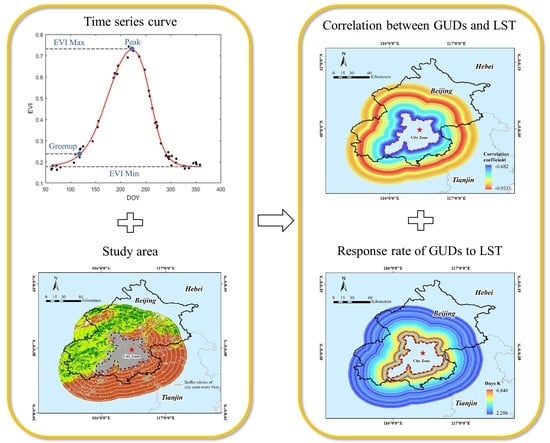
Vegetation GUDs show divergent correlations with LST according to vegetation types and distances away from the built-up areas, featuring a negative and relative weaker correlation near the urban area (0–10 km) than the surrounding area. GUDs are more sensitively correlated to LST in colder rings than in warmer rings;

(2)

The magnitude of ΔGUDs to ΔLST are positively correlated, with the advanced days in GUDs and the rising in LST both being larger near the urban domains when compared to these in rings 22 km further away from the urban perimeter, proving a solid influence of urban warming on the changes in vegetation GUDs;

(3)

The spatial pattern of the response rate of ΔGUDs to ΔLST demonstrated a distinct trend in different vegetations and distances, characterized by a distance-decay trend in forests and a downward trend first and then an upward trend in both grasslands and croplands. Higher sensitivity of ΔGUDs to ΔLST is identified in colder sites than in warmer rings, especially for croplands.

Although a detailed analysis about the relationships between vegetation GUDs and LST of forests, grasslands, and croplands were carried out at different distances away from the urban domain area, and some quantitative results were obtained, more efforts are needed to validate and consolidate the conclusions above by incorporating more vegetation types, climate factors, and other remote sensing data, such as the new MODIS LST product.

References

1. Zhang, R.; Qi, J.; Leng, S.; Wang, Q. Long-Term Vegetation Phenology Changes and Responses to Preseason Temperature and Precipitation in Northern China. Remote Sens. 2022, 14, 1396. [Google Scholar] [CrossRef]
2. Zhang, Y.; Yin, P.; Li, X.; Niu, Q.; Wang, Y.; Cao, W.; Huang, J.; Chen, H.; Yao, X.; Yu, L.; et al. The divergent response of vegetation phenology to urbanization: A case study of Beijing city, China. Sci. Total Environ. 2022, 803, 150079. [Google Scholar] [CrossRef] [PubMed]
3. Li, X.; Zhou, Y.; Asrar, G.R.; Meng, L. Characterizing spatiotemporal dynamics in phenology of urban ecosystems based on Landsat data. Sci. Total Environ. 2017, 605–606, 721–734. [Google Scholar] [CrossRef] [PubMed]
4. Krehbiel, C.; Zhang, X.; Henebry, G. Impacts of Thermal Time on Land Surface Phenology in Urban Areas. Remote Sens. 2017, 9, 499. [Google Scholar] [CrossRef] [Green Version]
5. Cao, R.; Shen, M.; Zhou, J.; Chen, J. Modeling vegetation green-up dates across the Tibetan Plateau by including both seasonal and daily temperature and precipitation. Agric. For. Meteorol. 2018, 249, 176–186. [Google Scholar] [CrossRef]
6. Forkel, M.; Migliavacca, M.; Thonicke, K.; Reichstein, M.; Schaphoff, S.; Weber, U.; Carvalhais, N. Codominant water control on global interannual variability and trends in land surface phenology and greenness. Glob. Chang. Biol. 2015, 21, 3414–3435. [Google Scholar] [CrossRef]
7. Jeong, S.-J.; Medvigy, D.; Shevliakova, E.; Malyshev, S. Uncertainties in terrestrial carbon budgets related to spring phenology. J. Geophys. Res. Biogeosci. 2012, 117. [Google Scholar] [CrossRef]
8. Keenan, T.F.; Gray, J.; Friedl, M.A.; Toomey, M.; Bohrer, G.; Hollinger, D.Y.; Munger, J.W.; O’Keefe, J.; Schmid, H.P.; Wing, I.S.; et al. Net carbon uptake has increased through warming-induced changes in temperate forest phenology. Nat. Clim. Chang. 2014, 4, 598–604. [Google Scholar] [CrossRef]
9. Richardson, A.D.; Keenan, T.F.; Migliavacca, M.; Ryu, Y.; Sonnentag, O.; Toomey, M. Climate change, phenology, and phenological control of vegetation feedbacks to the climate system. Agric. For. Meteorol. 2013, 169, 156–173. [Google Scholar] [CrossRef]
10. Wu, C.; Hou, X.; Peng, D.; Gonsamo, A.; Xu, S. Land surface phenology of China’s temperate ecosystems over 1999–2013: Spatial–temporal patterns, interaction effects, covariation with climate and implications for productivity. Agric. For. Meteorol. 2016, 216, 177–187. [Google Scholar] [CrossRef]
11. Körner, C.; Basler, D. Phenology under global warming. Science 2010, 327, 1461–1462. [Google Scholar] [CrossRef] [PubMed]
12. Vitasse, Y.; François, C.; Delpierre, N.; Dufrêne, E.; Kremer, A.; Chuine, I.; Delzon, S. Assessing the effects of climate change on the phenology of European temperate trees. Agric. For. Meteorol. 2011, 151, 969–980. [Google Scholar] [CrossRef]
13. Zheng, Z.; Zhu, W.; Chen, G.; Jiang, N.; Fan, D.; Zhang, D. Continuous but diverse advancement of spring-summer phenology in response to climate warming across the Qinghai-Tibetan Plateau. Agric. For. Meteorol. 2016, 223, 194–202. [Google Scholar] [CrossRef]
14. Liu, Y.; Wu, C.; Peng, D.; Xu, S.; Gonsamo, A.; Jassal, R.S.; Altaf Arain, M.; Lu, L.; Fang, B.; Chen, J.M. Improved modeling of land surface phenology using MODIS land surface reflectance and temperature at evergreen needleleaf forests of central North America. Remote Sens. Environ. 2016, 176, 152–162. [Google Scholar] [CrossRef]
15. Barr, A.; Black, T.A.; McCaughey, H. Climatic and Phenological Controls of the Carbon and Energy Balances of Three Contrasting Boreal Forest Ecosystems in Western Canada. In Phenology of Ecosystem Processes; Springer: Cham, Switzerland, 2009; pp. 3–34. [Google Scholar] [CrossRef]
16. Ren, S.; Li, Y.; Peichl, M. Diverse effects of climate at different times on grassland phenology in mid-latitude of the Northern Hemisphere. Ecol. Indic. 2020, 113, 106260. [Google Scholar] [CrossRef]
17. Guo, L.; Gao, J.; Hao, C.; Zhang, L.; Wu, S.; Xiao, X. Winter Wheat Green-up Date Variation and its Diverse Response on the Hydrothermal Conditions over the North China Plain, Using MODIS Time-Series Data. Remote Sens. 2019, 11, 1593. [Google Scholar] [CrossRef] [Green Version]
18. Zhou, D.; Zhao, S.; Zhang, L.; Liu, S. Remotely sensed assessment of urbanization effects on vegetation phenology in China’s 32 major cities. Remote Sens. Environ. 2016, 176, 272–281. [Google Scholar] [CrossRef] [Green Version]
19. Seto, K.C.; Fragkias, M.; Guneralp, B.; Reilly, M.K. A meta-analysis of global urban land expansion. PLoS ONE 2011, 6, e23777. [Google Scholar] [CrossRef]
20. Seto, K.C.; Guneralp, B.; Hutyra, L.R. Global forecasts of urban expansion to 2030 and direct impacts on biodiversity and carbon pools. Proc. Natl. Acad. Sci. USA 2012, 109, 16083–16088. [Google Scholar] [CrossRef] [Green Version]
21. Nations, U. World Urbanization Prospects: The 2014 Revision: Highlights; Department of Economic and Social Affairs, Population Division: New York, NY, USA, 2014. [Google Scholar] [CrossRef] [Green Version]
22. Ji, Y.; Jin, J.; Zhan, W.; Guo, F.; Yan, T. Quantification of Urban Heat Island-Induced Contribution to Advance in Spring Phenology: A Case Study in Hangzhou, China. Remote Sens. 2021, 13, 3684. [Google Scholar] [CrossRef]
23. Jia, W.; Zhao, S.; Liu, S. Vegetation growth enhancement in urban environments of the Conterminous United States. Glob. Chang. Biol. 2018, 24, 4084–4094. [Google Scholar] [CrossRef] [PubMed]
24. Li, X.; Zhou, Y.; Asrar, G.R.; Mao, J.; Li, X.; Li, W. Response of vegetation phenology to urbanization in the conterminous United States. Glob. Chang. Biol. 2017, 23, 2818–2830. [Google Scholar] [CrossRef] [PubMed]
25. Ren, Q.; He, C.; Huang, Q.; Zhou, Y. Urbanization Impacts on Vegetation Phenology in China. Remote Sens. 2018, 10, 1905. [Google Scholar] [CrossRef] [Green Version]
26. Li, D.; Stucky, B.J.; Deck, J.; Baiser, B.; Guralnick, R.P. The effect of urbanization on plant phenology depends on regional temperature. Nat. Ecol. Evol. 2019, 3, 1661–1667. [Google Scholar] [CrossRef] [PubMed]
27. Tian, J.; Zhu, X.; Shen, Z.; Wu, J.; Xu, S.; Liang, Z.; Wang, J. Investigating the urban-induced microclimate effects on winter wheat spring phenology using Sentinel-2 time series. Agric. For. Meteorol. 2020, 294. [Google Scholar] [CrossRef]
28. Yuan, M.; Zhao, L.; Lin, A.; Li, Q.; She, D.; Qu, S. How do climatic and non-climatic factors contribute to the dynamics of vegetation autumn phenology in the Yellow River Basin, China? Ecol. Indic. 2020, 112. [Google Scholar] [CrossRef]
29. Wang, S.; Ju, W.; Penuelas, J.; Cescatti, A.; Zhou, Y.; Fu, Y.; Huete, A.; Liu, M.; Zhang, Y. Urban-rural gradients reveal joint control of elevated CO2 and temperature on extended photosynthetic seasons. Nat. Ecol. Evol. 2019, 3, 1076–1085. [Google Scholar] [CrossRef] [Green Version]
30. Luo, Z.; Sun, O.J.; Ge, Q.; Xu, W.; Zheng, J. Phenological responses of plants to climate change in an urban environment. Ecol. Res. 2006, 22, 507–514. [Google Scholar] [CrossRef]
31. Zhang, X.; Friedl, M.A.; Schaaf, C.B.; Strahler, A.H.; Schneider, A. The footprint of urban climates on vegetation phenology. Geophys. Res. Lett. 2004, 31. [Google Scholar] [CrossRef]
32. Jochner, S.C.; Sparks, T.H.; Estrella, N.; Menzel, A. The influence of altitude and urbanisation on trends and mean dates in phenology (1980–2009). Int. J. Biometeorol. 2012, 56, 387–394. [Google Scholar] [CrossRef]
33. Wang, X.; Gao, Q.; Wang, C.; Yu, M. Spatiotemporal patterns of vegetation phenology change and relationships with climate in the two transects of East China. Glob. Ecol. Conserv. 2017, 10, 206–219. [Google Scholar] [CrossRef]
34. Peng, D.; Wu, C.; Li, C.; Zhang, X.; Liu, Z.; Ye, H.; Luo, S.; Liu, X.; Hu, Y.; Fang, B. Spring green-up phenology products derived from MODIS NDVI and EVI: Intercomparison, interpretation and validation using National Phenology Network and AmeriFlux observations. Ecol. Indic. 2017, 77, 323–336. [Google Scholar] [CrossRef]
35. Zhang, X.; Friedl, M.; Schaaf, C.B.; Strahler, A.H.; Hodges, J.C.F.; Gao, F.; Reed, B.C.; Huete, A. Monitoring vegetation phenology using MODIS. Remote Sens. Environ. 2003, 84, 471–475. [Google Scholar] [CrossRef]
36. Moon, M.; Zhang, X.; Henebry, G.M.; Liu, L.; Gray, J.M.; Melaas, E.K.; Friedl, M.A. Long-term continuity in land surface phenology measurements: A comparative assessment of the MODIS land cover dynamics and VIIRS land surface phenology products. Remote Sens. Environ. 2019, 226, 74–92. [Google Scholar] [CrossRef]
37. Jochner, S.; Menzel, A. Urban phenological studies—Past, present, future. Environ. Pollut 2015, 203, 250–261. [Google Scholar] [CrossRef]
38. Wu, J. Urban ecology and sustainability: The state-of-the-science and future directions. Landsc. Urban Plan. 2014, 125, 209–221. [Google Scholar] [CrossRef]
39. Li, P.; Sun, M.; Liu, Y.; Ren, P.; Peng, C.; Zhou, X.; Tang, J. Response of Vegetation Photosynthetic Phenology to Urbanization in Dongting Lake Basin, China. Remote Sens. 2021, 13, 3722. [Google Scholar] [CrossRef]
40. Qiu, T.; Song, C.; Zhang, Y.; Liu, H.; Vose, J.M. Urbanization and climate change jointly shift land surface phenology in the northern mid-latitude large cities. Remote Sens. Environ. 2020, 236, 111477. [Google Scholar] [CrossRef]
41. Su, Y.; Wang, X.; Wang, X.; Cui, B.; Sun, X. Leaf and male cone phenophases of Chinese pine (Pinus tabulaeformis Carr.) along a rural-urban gradient in Beijing, China. Urban For. Urban Green. 2019, 42, 61–71. [Google Scholar] [CrossRef]
42. Xing, Q.; Sun, Z.; Tao, Y.; Shang, J.; Miao, S.; Xiao, C.; Zheng, C. Projections of future temperature-related cardiovascular mortality under climate change, urbanization and population aging in Beijing, China. Environ. Int. 2022, 163, 107231. [Google Scholar] [CrossRef]
43. Chen, W.; Zhang, Y.; Gao, W.; Zhou, D. The Investigation of Urbanization and Urban Heat Island in Beijing Based on Remote Sensing. Procedia Soc. Behav. Sci. 2016, 216, 141–150. [Google Scholar] [CrossRef] [Green Version]
44. Li, X.; Gong, P.; Liang, L. A 30-year (1984–2013) record of annual urban dynamics of Beijing City derived from Landsat data. Remote Sens. Environ. 2015, 166, 78–90. [Google Scholar] [CrossRef]
45. Wu, C.; Peng, D.; Soudani, K.; Siebicke, L.; Gough, C.M.; Arain, M.A.; Bohrer, G.; Lafleur, P.M.; Peichl, M.; Gonsamo, A.; et al. Land surface phenology derived from normalized difference vegetation index (NDVI) at global FLUXNET sites. Agric. For. Meteorol. 2017, 233, 171–182. [Google Scholar] [CrossRef]
46. Richardson, A.D.; Hufkens, K.; Milliman, T.; Frolking, S. Intercomparison of phenological transition dates derived from the PhenoCam Dataset V1.0 and MODIS satellite remote sensing. Sci. Rep. 2018, 8, 5679. [Google Scholar] [CrossRef] [PubMed] [Green Version]
47. Liang, L.; Schwartz, M.D.; Fei, S. Validating satellite phenology through intensive ground observation and landscape scaling in a mixed seasonal forest. Remote Sens. Environ. 2011, 115, 143–157. [Google Scholar] [CrossRef]
48. Ganguly, S.; Friedl, M.A.; Tan, B.; Zhang, X.; Verma, M. Land surface phenology from MODIS: Characterization of the Collection 5 global land cover dynamics product. Remote Sens. Environ. 2010, 114, 1805–1816. [Google Scholar] [CrossRef] [Green Version]
49. Gray, J.; Sulla-Menashe, D.; Friedl, M.A. User Guide to Collection 6 MODIS Land Cover Dynamics (MCD12Q2) Product. 2019. Available online: https://lpdaac.usgs.gov/products/mcd12q2v006/ (accessed on 15 January 2019).
50. Meng, L.; Mao, J.; Zhou, Y.; Richardson, A.D.; Lee, X.; Thornton, P.E.; Ricciuto, D.M.; Li, X.; Dai, Y.; Shi, X.; et al. Urban warming advances spring phenology but reduces the response of phenology to temperature in the conterminous United States. Proc. Natl. Acad. Sci. USA 2020, 117, 4228–4233. [Google Scholar] [CrossRef]
51. Buyantuyev, A.; Wu, J. Urbanization diversifies land surface phenology in arid environments: Interactions among vegetation, climatic variation, and land use pattern in the Phoenix metropolitan region, USA. Landsc. Urban Plan. 2012, 105, 149–159. [Google Scholar] [CrossRef]
52. Zipper, S.C.; Schatz, J.; Singh, A.; Kucharik, C.J.; Townsend, P.A.; Loheide, S.P. Urban heat island impacts on plant phenology: Intra-urban variability and response to land cover. Environ. Res. Lett. 2016, 11, 054023. [Google Scholar] [CrossRef]
53. Krehbiel, C.; Henebry, G. A Comparison of Multiple Datasets for Monitoring Thermal Time in Urban Areas over the U.S. Upper Midwest. Remote Sens. 2016, 8, 297. [Google Scholar] [CrossRef] [Green Version]
54. Shen, M.; Piao, S.; Chen, X.; An, S.; Fu, Y.H.; Wang, S.; Cong, N.; Janssens, I.A. Strong impacts of daily minimum temperature on the green-up date and summer greenness of the Tibetan Plateau. Glob. Chang. Biol. 2016, 22, 3057–3066. [Google Scholar] [CrossRef] [PubMed]
55. Cannell, M.; Smith, R. Thermal time, chill days and prediction of budburst in picea sitchensis. J. Appl. Ecol. 1893, 20, 951–963. [Google Scholar] [CrossRef]
56. Stocker, T.F.; Qin, D.; Plattner, G.K.; Tignor, M.; Allen, S.K.; Boschung, J.; Nauels, A.; Xia, Y.; Bex, V.; Midgley, P.M. Climate Change 2013: The Physical Science Basis; Contribution of Working Group I to the Fifth Assessment Report of IPCC the Intergovernmental Panel on Climate Change; IPCC: Geneva, Switzerland, 2014. [Google Scholar] [CrossRef] [Green Version]
57. Cong, N.; Piao, S.; Chen, A.; Wang, X.; Lin, X.; Chen, S.; Han, S.; Zhou, G.; Zhang, X. Spring vegetation green-up date in China inferred from SPOT NDVI data: A multiple model analysis. Agric. For. Meteorol. 2012, 165, 104–113. [Google Scholar] [CrossRef]
58. Garonna, I.; de Jong, R.; de Wit, A.J.; Mucher, C.A.; Schmid, B.; Schaepman, M.E. Strong contribution of autumn phenology to changes in satellite-derived growing season length estimates across Europe (1982–2011). Glob. Chang. Biol. 2014, 20, 3457–3470. [Google Scholar] [CrossRef] [PubMed]
59. Zhu, X.; Duan, S.-B.; Li, Z.-L.; Zhao, W.; Wu, H.; Leng, P.; Gao, M.; Zhou, X. Retrieval of Land Surface Temperature with Topographic Effect Correction from Landsat 8 Thermal Infrared Data in Mountainous Areas. IEEE Trans. Geosci. Remote Sens. 2021, 59, 6674–6687. [Google Scholar] [CrossRef]
60. Hao, D.; Bisht, G.; Gu, Y.; Lee, W.; Leung, L.R. A Parameterization of Sub-grid Topographical Effects on Solar Radiation in the E3SM Land Model (Version 1.0): Implementation and Evaluation over the Tibetan Plateau. Copernic. GmbH 2021, 14, 6273–6289. [Google Scholar] [CrossRef]
61. Prevey, J.; Vellend, M.; Ruger, N.; Hollister, R.D.; Bjorkman, A.D.; Myers-Smith, I.H.; Elmendorf, S.C.; Clark, K.; Cooper, E.J.; Elberling, B.; et al. Greater temperature sensitivity of plant phenology at colder sites: Implications for convergence across northern latitudes. Glob. Chang. Biol. 2017, 23, 2660–2671. [Google Scholar] [CrossRef] [Green Version]
Figure 1. The delineation of study area.
Remotesensing 14 02788 g001
Figure 2. The delineation of 25 ring zones along the built-up area of Beijing.
Remotesensing 14 02788 g002
Figure 3. Schema for data analysis.
Remotesensing 14 02788 g003
Figure 4. Spatial patterns of 19-year average (a) green-up dates and (c) land surface temperature over the period 2001–2019 and the area percentage charts for different GUDs (b) and LST (d).
Remotesensing 14 02788 g004
Figure 5. Correlation between average GUDs and average LST of forests (a), grasslands (b), and croplands (c) over the period 2001–2019.
Remotesensing 14 02788 g005
Figure 6. Spatial patterns of correlation between vegetation GUDs and LST in forests (a,b), grasslands (c,d), and croplands (e,f) along the urban-rural gradient for the period 2001–2019.
Remotesensing 14 02788 g006
Figure 8. Spatial pattern of the response rate of absolute ΔGUDs to ΔLST in forests (a,b), grasslands (c,d), and croplands (e,f) along the urban-rural gradient.
Remotesensing 14 02788 g008
Figure 9. The relationship of vegetation green-up dates (GUDs) to daytime and nighttime land surface temperatures (LST) along the urban-rural gradient.
Remotesensing 14 02788 g009aRemotesensing 14 02788 g009b
Publisher’s Note: MDPI stays neutral with regard to jurisdictional claims in published maps and institutional affiliations.